
Stability Analysis on the Moon’s Rotation in a Perturbed Binary Asteroid


Abstract
1. Introduction
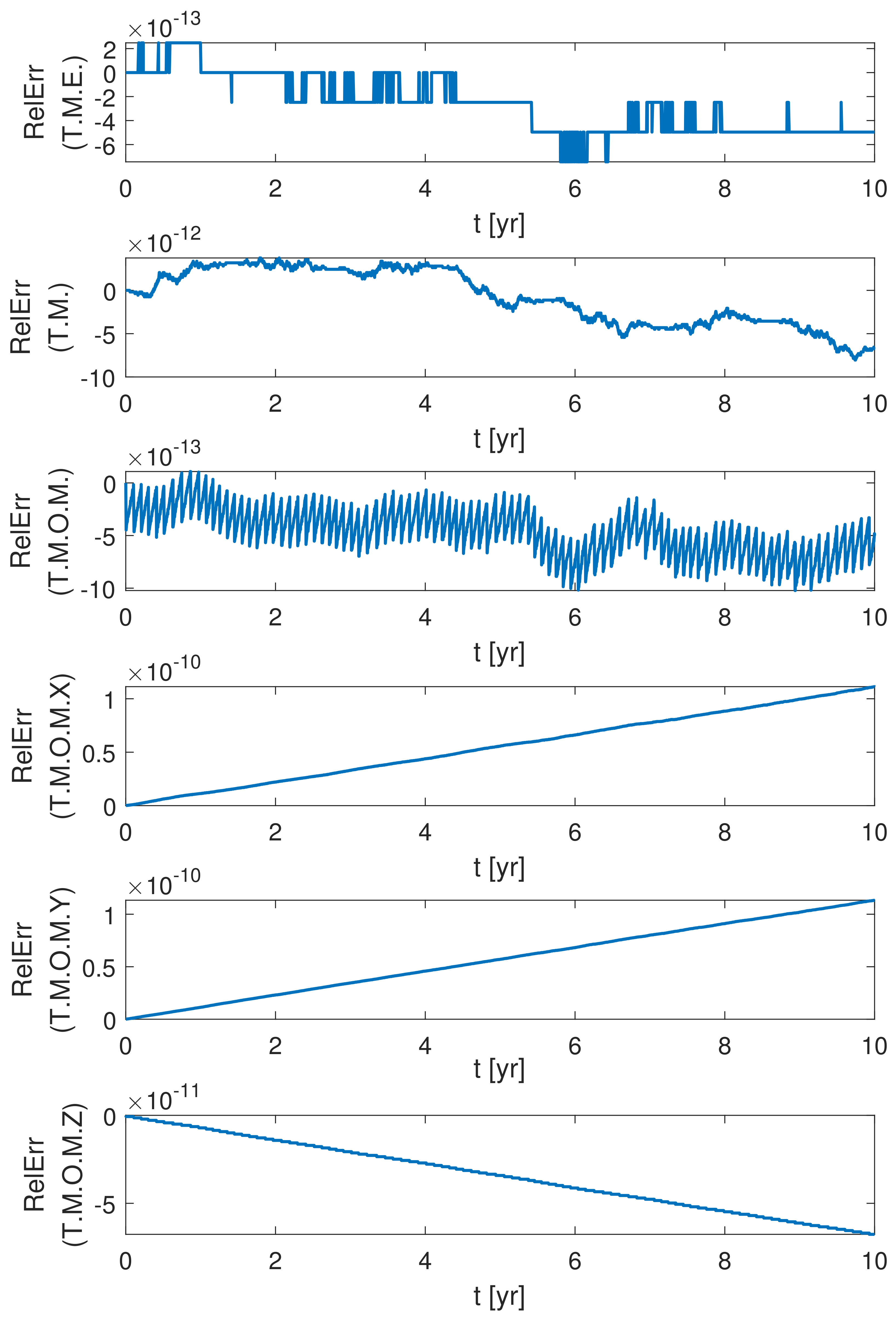
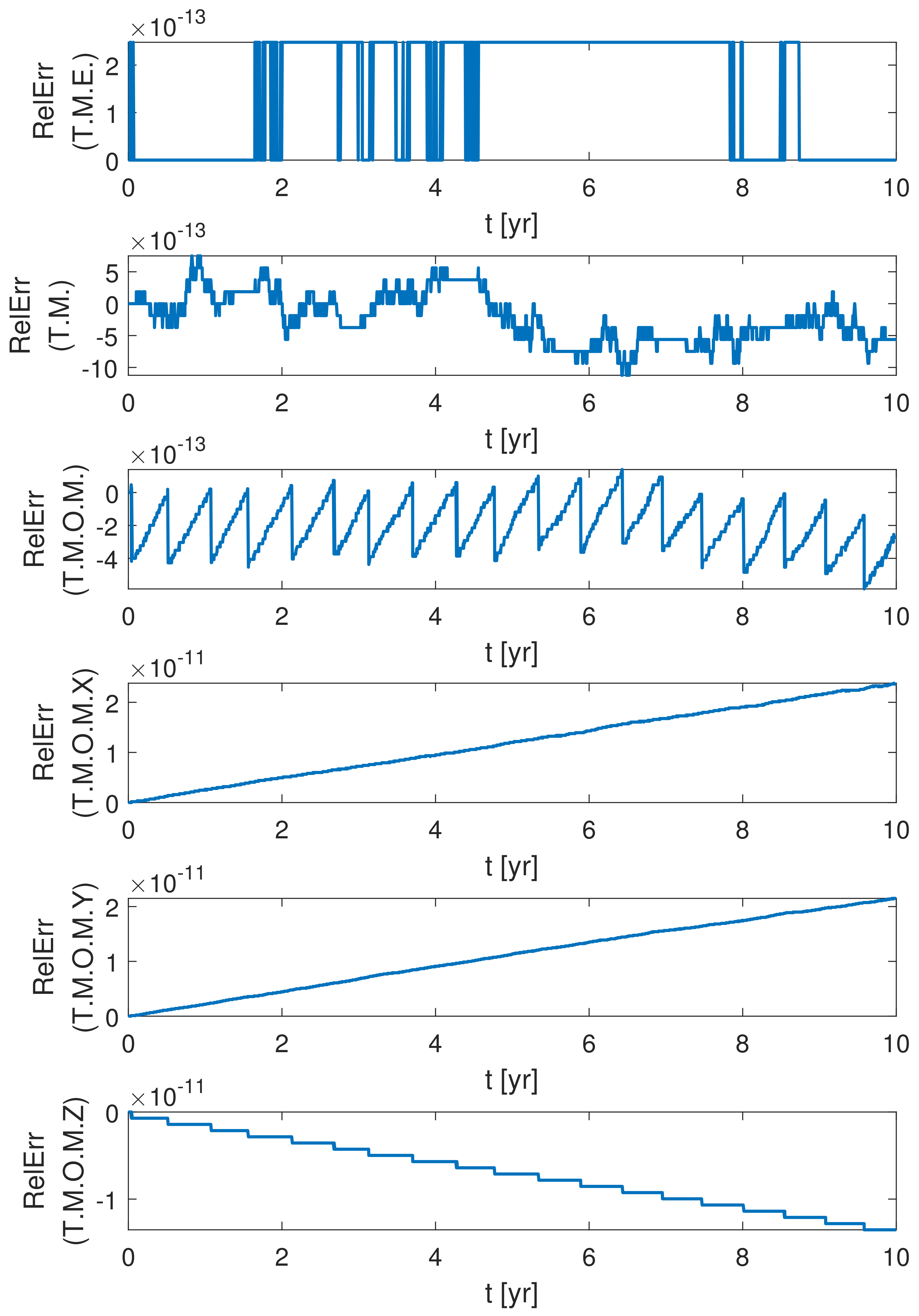
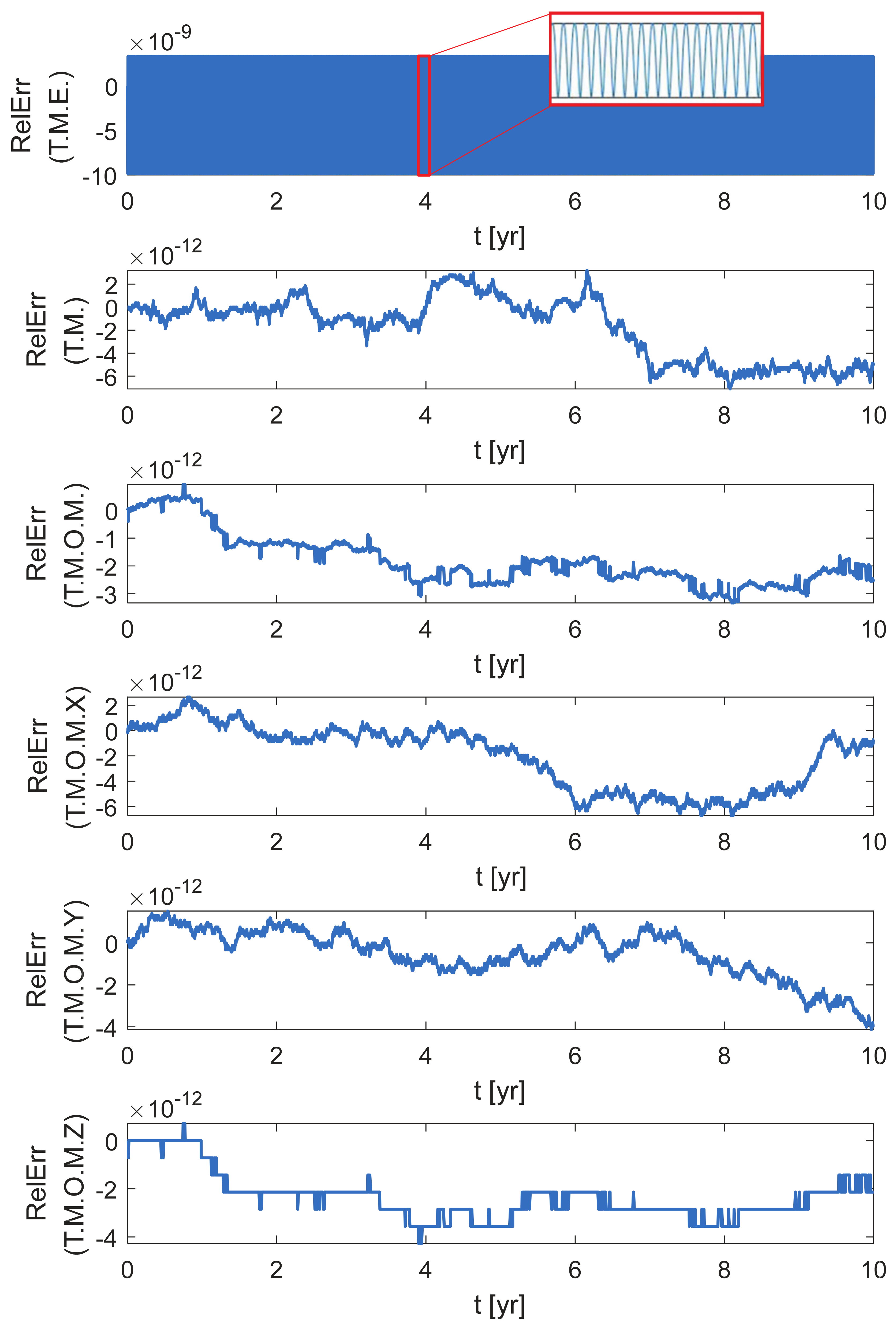
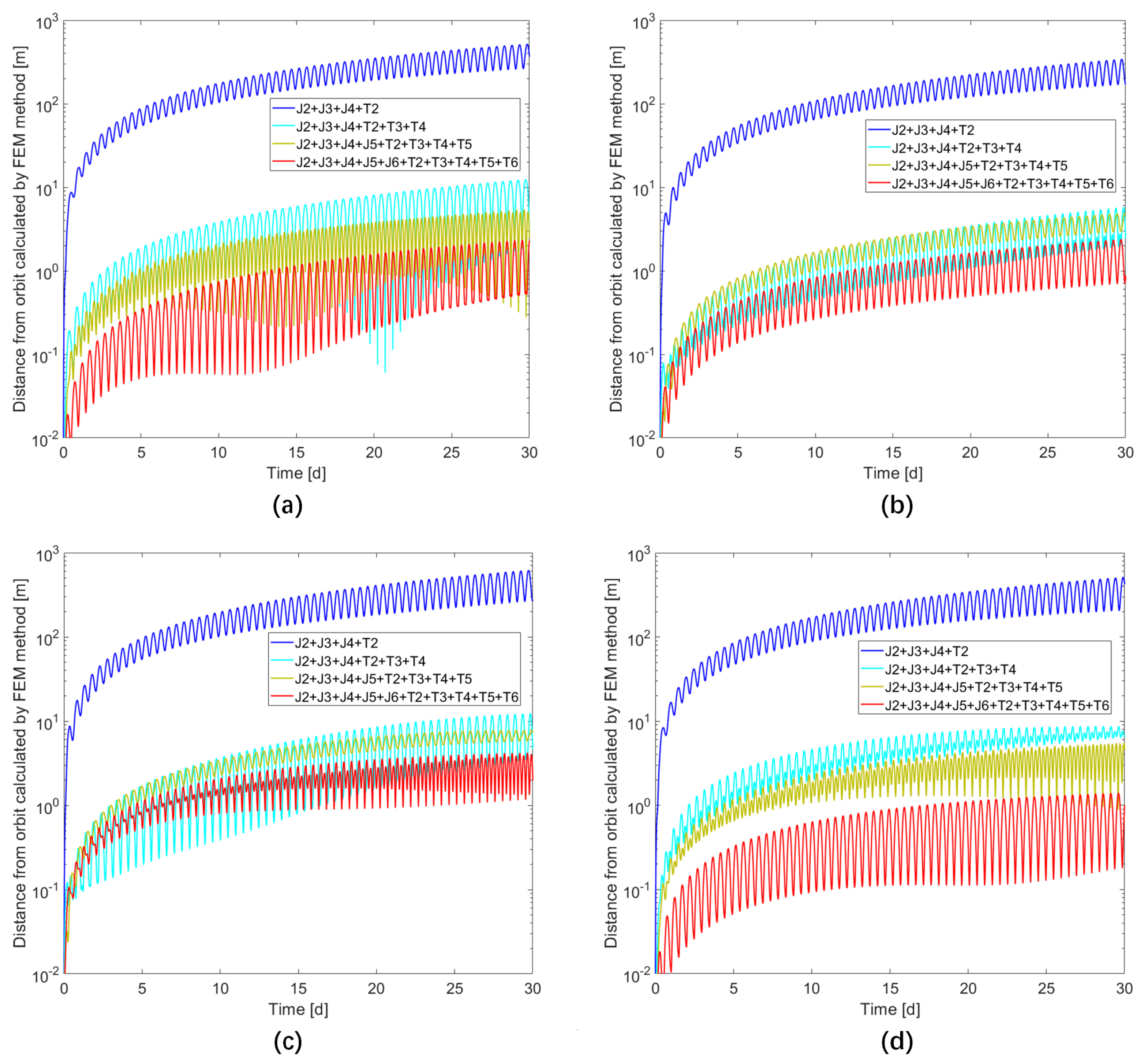
2. Comparison of Numerical Schemes for Long Assessment
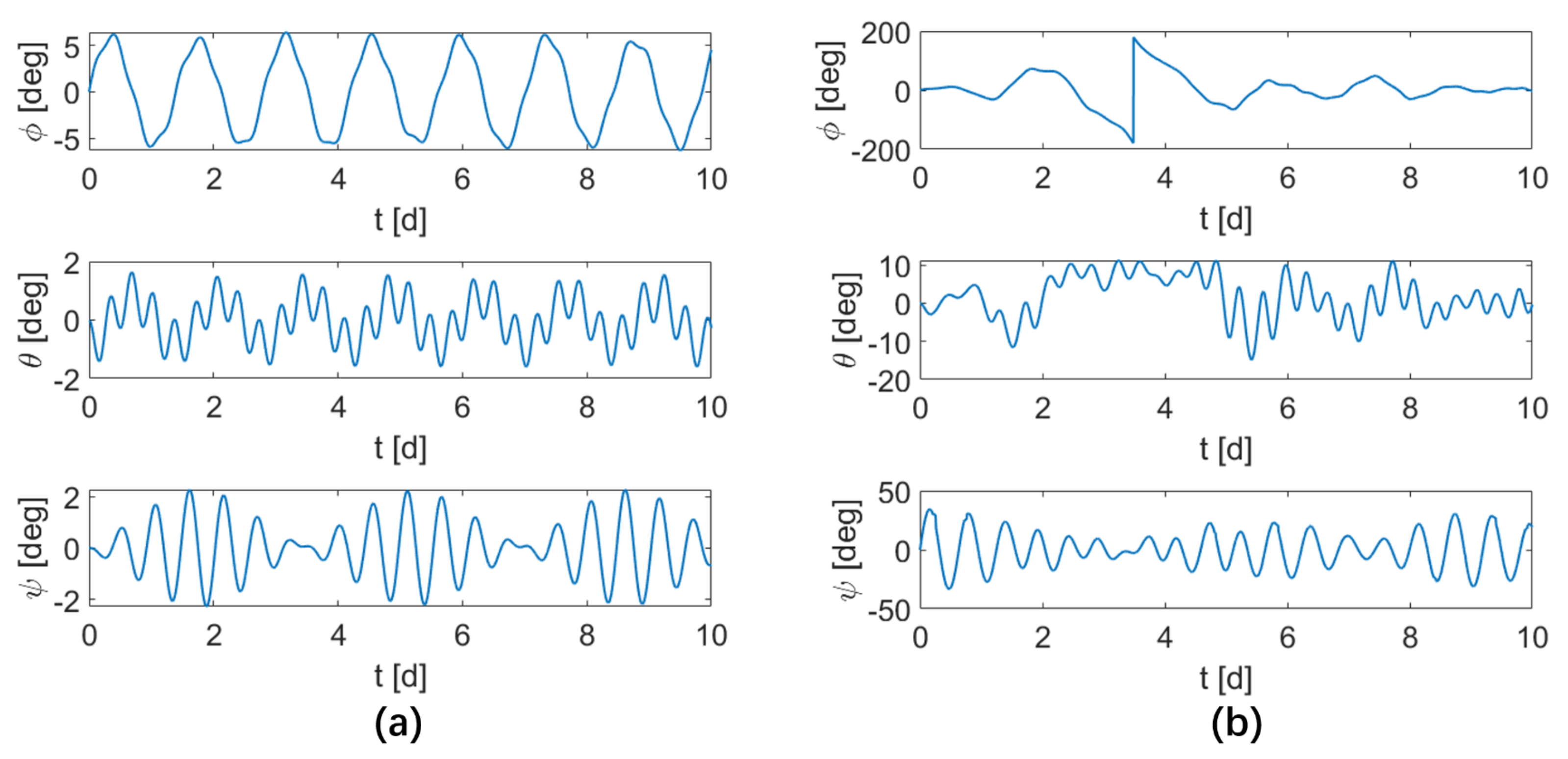
3. Stability of the Excited Spin State of the Secondary
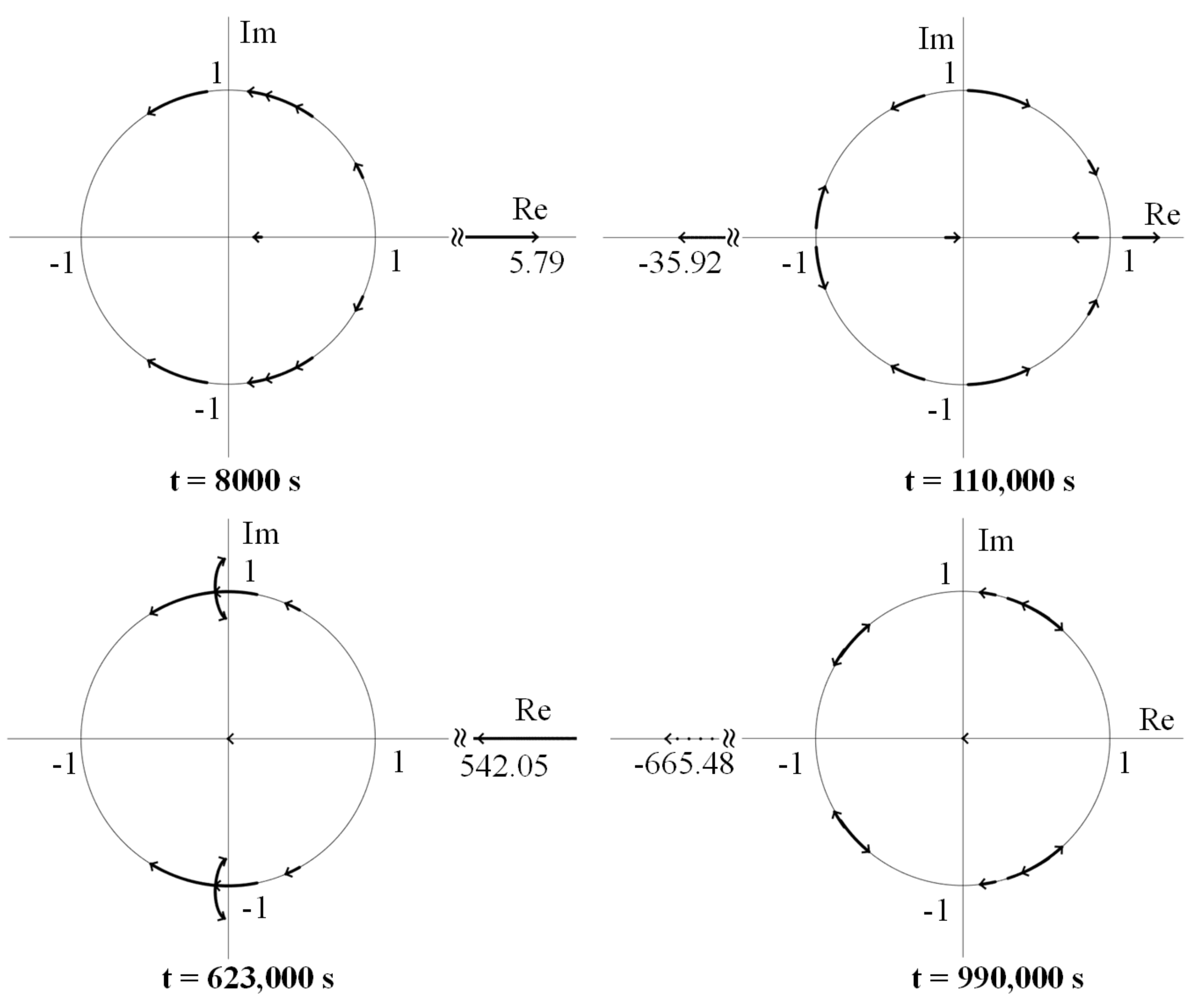
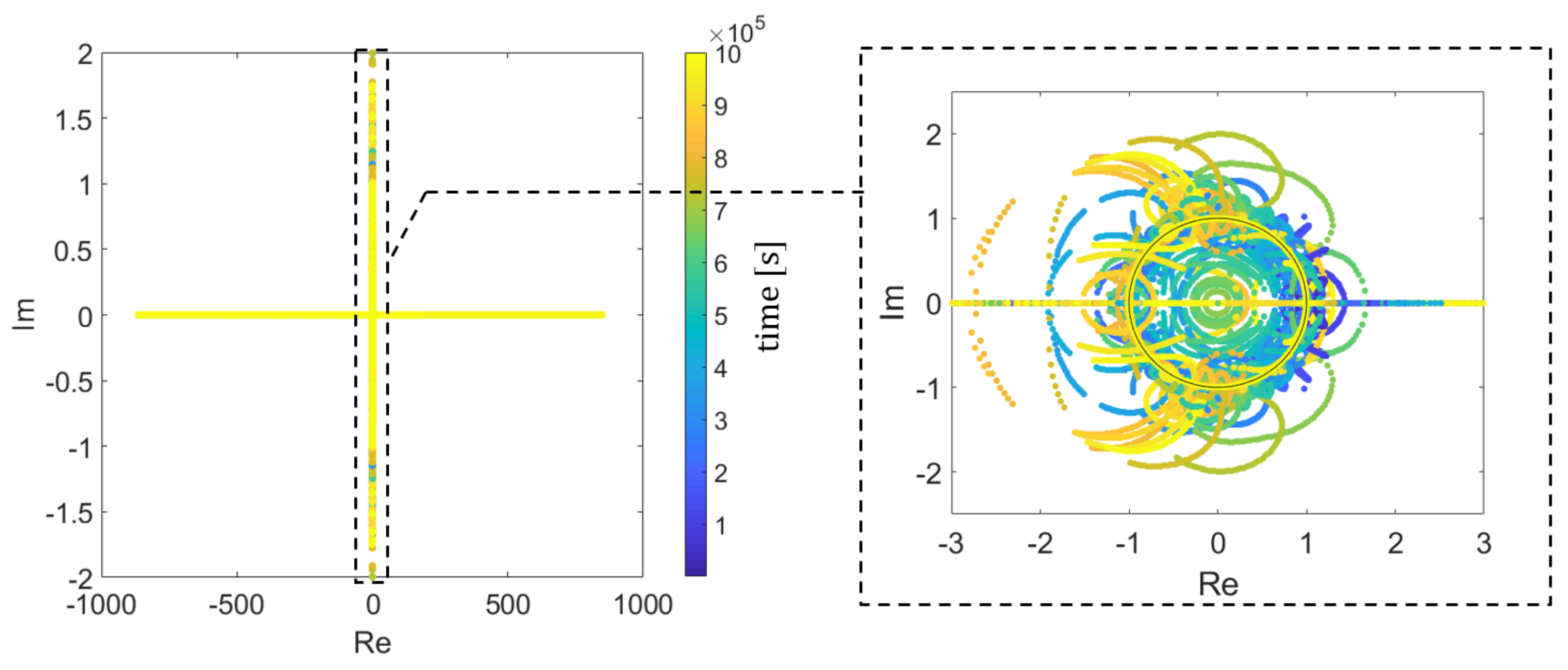
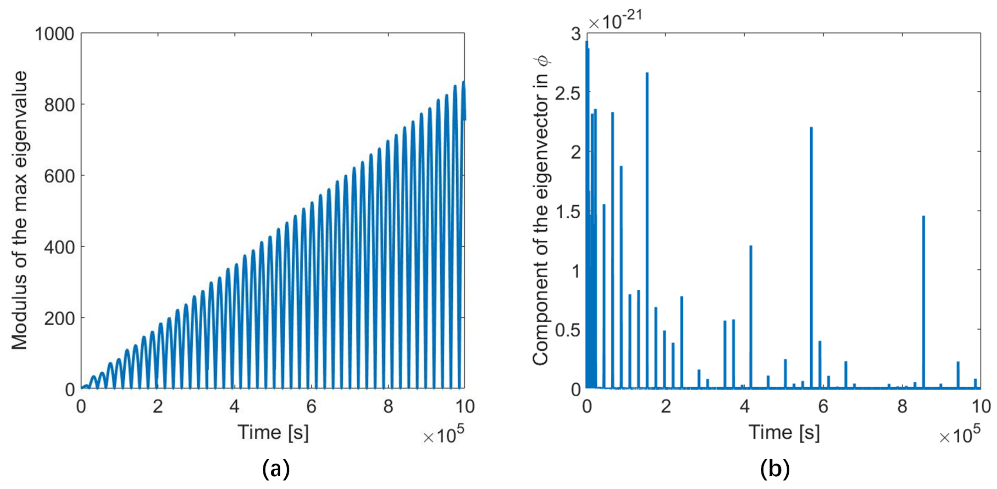
3.1. Definition of the Linearised Error Propagation Matrix
3.2. Analysis of with the Initial Angular Velocity from to
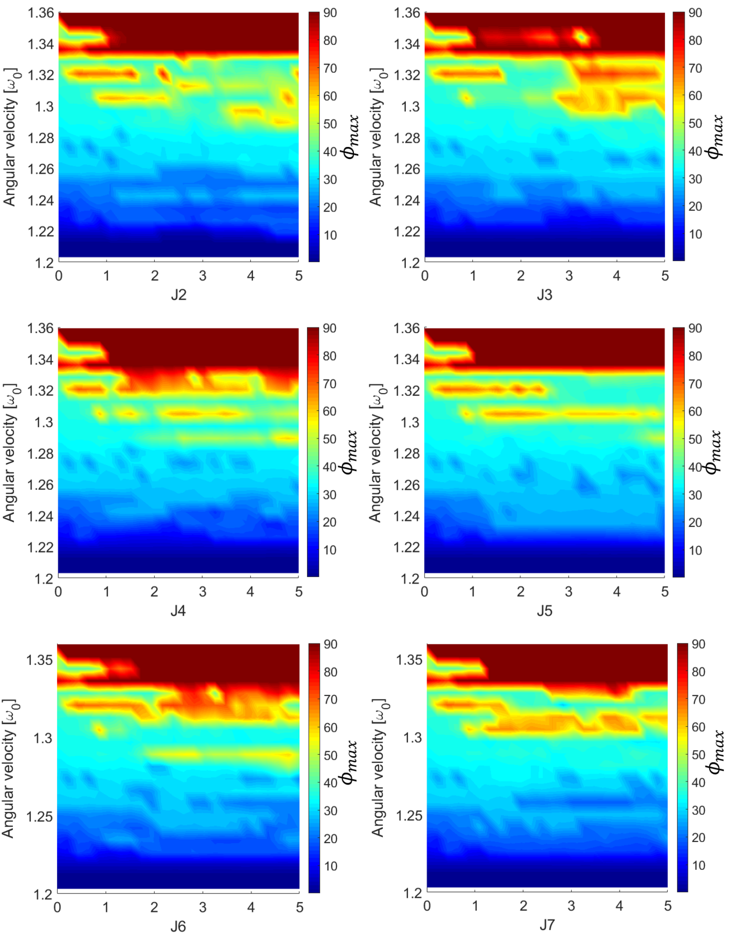
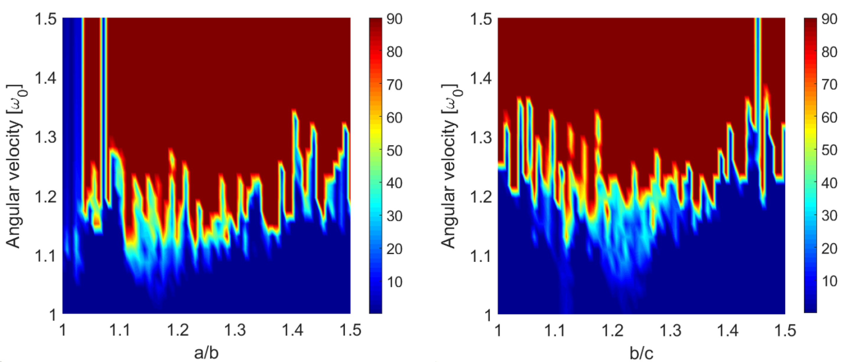
3.3. Effect of the Non-Spherical Gravitational Field of the Primary and the Shape of the Secondary on the Tumbling Motion of the Secondary
4. Conclusions
Author Contributions
Funding
Data Availability Statement
Acknowledgments
Conflicts of Interest
Appendix A


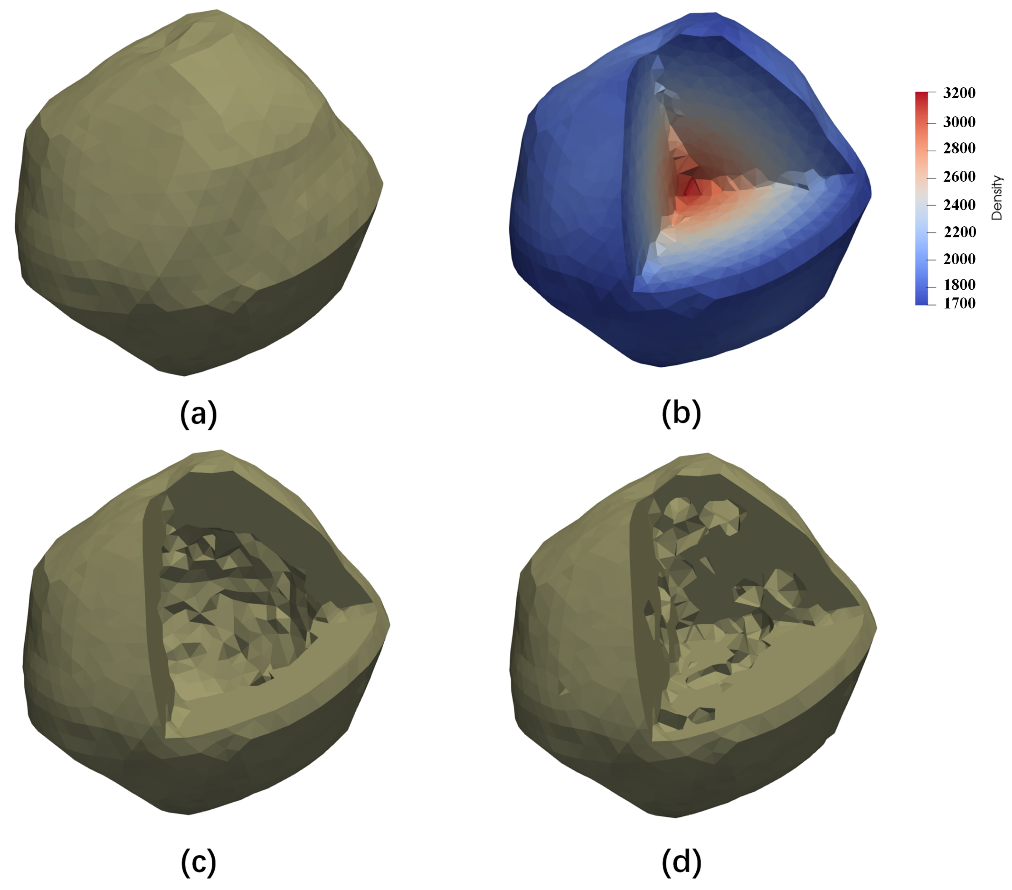
| Model (a) | Model (b) | Model (c) | Model (d) | |
|---|---|---|---|---|

References
- Cheng, A.; Michel, P.; Jutzi, M.; Rivkin, A.; Stickle, A.; Barnouin, O.; Ernst, C.; Atchison, J.; Pravec, P.; Richardson, D.; et al. Asteroid impact & deflection assessment mission: Kinetic impactor. Planet. Space Sci. 2016, 121, 27–35. [Google Scholar]
- Michel, P.; Cheng, A.; Küppers, M.; Pravec, P.; Blum, J.; Delbo, M.; Green, S.; Rosenblatt, P.; Tsiganis, K.; Vincent, J.B.; et al. Science case for the asteroid impact mission (AIM): A component of the asteroid impact & deflection assessment (AIDA) mission. Adv. Space Res. 2016, 57, 2529–2547. [Google Scholar]
- Cheng, A.F.; Rivkin, A.S.; Michel, P.; Atchison, J.; Barnouin, O.; Benner, L.; Chabot, N.L.; Ernst, C.; Fahnestock, E.G.; Kueppers, M.; et al. AIDA DART asteroid deflection test: Planetary defense and science objectives. Planet. Space Sci. 2018, 157, 104–115. [Google Scholar] [CrossRef]
- Rainey, E.S.; Stickle, A.M.; Cheng, A.F.; Rivkin, A.S.; Chabot, N.L.; Barnouin, O.S.; Ernst, C.M.; Group, A.I.S.W. Impact Modeling for the Double Asteroid Redirection Test Mission. In Proceedings of the Hypervelocity Impact Symposium, Destin, FL, USA, 16–20 April 2019; Volume 883556, p. HVIS2019-038. [Google Scholar]
- Rainey, E.S.; Stickle, A.M.; Cheng, A.F.; Rivkin, A.S.; Chabot, N.L.; Barnouin, O.S.; Ernst, C.M.; AIDA/DART Impact Simulation Working Group. Impact modeling for the Double Asteroid Redirection Test (DART) mission. Int. J. Impact Eng. 2020, 142, 103528. [Google Scholar] [CrossRef]
- Rivkin, A.S.; Chabot, N.L.; Stickle, A.M.; Thomas, C.A.; Richardson, D.C.; Barnouin, O.; Fahnestock, E.G.; Ernst, C.M.; Cheng, A.F.; Chesley, S.; et al. The double asteroid redirection test (DART): Planetary defense investigations and requirements. Planet. Sci. J. 2021, 2, 173. [Google Scholar] [CrossRef]
- Agrusa, H.; Richardson, D.; Barbee, B.; Bottke, W.; Cheng, A.; Eggl, S.; Ferrari, F.; Hirabayashi, M.; Karatekin, O.; McMahon, J.; et al. Predictions for the Dynamical State of the Didymos System Before and After the Planned DART Impact. LPI Contrib. 2022, 2678, 2447. [Google Scholar]
- Agrusa, H.F.; Gkolias, I.; Tsiganis, K.; Richardson, D.C.; Meyer, A.J.; Scheeres, D.J.; Ćuk, M.; Jacobson, S.A.; Michel, P.; Karatekin, Ö.; et al. The excited spin state of Dimorphos resulting from the DART impact. Icarus 2021, 370, 114624. [Google Scholar] [CrossRef]
- Agrusa, H.; Ballouz, R.; Meyer, A.J.; Tasev, E.; Noiset, G.; Karatekin, Ö.; Michel, P.; Richardson, D.C.; Hirabayashi, M. Rotation-induced granular motion on the secondary component of binary asteroids: Application to the DART impact on Dimorphos. Astron. Astrophys. 2022, 664, L3. [Google Scholar] [CrossRef]
- Werner, R.A.; Scheeres, D.J. Mutual potential of homogeneous polyhedra. Celest. Mech. Dyn. Astron. 2005, 91, 337–349. [Google Scholar] [CrossRef]
- Hirabayashi, M.; Scheeres, D.J. Recursive computation of mutual potential between two polyhedra. Celest. Mech. Dyn. Astron. 2013, 117, 245–262. [Google Scholar] [CrossRef]
- Hou, X.; Scheeres, D.J.; Xin, X. Mutual potential between two rigid bodies with arbitrary shapes and mass distributions. Celest. Mech. Dyn. Astron. 2017, 127, 369–395. [Google Scholar] [CrossRef]
- Richardson, D.C.; Quinn, T.; Stadel, J.; Lake, G. Direct large-scale N-body simulations of planetesimal dynamics. Icarus 2000, 143, 45–59. [Google Scholar] [CrossRef]
- Yu, Y.; Cheng, B.; Hayabayashi, M.; Michel, P.; Baoyin, H. A finite element method for computational full two-body problem: I. The mutual potential and derivatives over bilinear tetrahedron elements. Celest. Mech. Dyn. Astron. 2019, 131, 51. [Google Scholar] [CrossRef]
- Ruth, R.D. A canonical integration technique. IEEE Trans. Nucl. Sci. 1983, 30, 2669–2671. [Google Scholar] [CrossRef]
- Marsden, J.E.; West, M. Discrete mechanics and variational integrators. Acta Numer. 2001, 10, 357–514. [Google Scholar] [CrossRef]
- Feng, K.; Qin, M. Symplectic Geometric Algorithms for Hamiltonian Systems; Springer: Berlin/Heidelberg, Germany, 2010; Volume 449. [Google Scholar]
- Karamali, G.; Shiri, B. Numerical solution of higher index DAEs using their IAE’s structure: Trajectory-prescribed path control problem and simple pendulum. Casp. J. Math. Sci. CJMS 2018, 7, 1–15. [Google Scholar]
- Kosmas, O.T.; Vlachos, D. Phase-fitted discrete Lagrangian integrators. Comput. Phys. Commun. 2010, 181, 562–568. [Google Scholar] [CrossRef]
- Kosmas, O.T.; Vlachos, D. Local path fitting: A new approach to variational integrators. J. Comput. Appl. Math. 2012, 236, 2632–2642. [Google Scholar] [CrossRef]
- Kosmas, O.; Leyendecker, S. Analysis of higher order phase fitted variational integrators. Adv. Comput. Math. 2016, 42, 605–619. [Google Scholar] [CrossRef]
- Kosmas, O.; Leyendecker, S. Variational integrators for orbital problems using frequency estimation. Adv. Comput. Math. 2019, 45, 1–21. [Google Scholar] [CrossRef]
- Kosmas, O. Energy minimization scheme for split potential systems using exponential variational integrators. Appl. Mech. 2021, 2, 431–441. [Google Scholar] [CrossRef]
- Leimkuhler, B.; Reich, S. Simulating Hamiltonian Dynamics; Cambridge University Press: Cambridge, UK, 2004; Number 14. [Google Scholar]
- Dullweber, A.; Leimkuhler, B.; McLachlan, R. Symplectic splitting methods for rigid body molecular dynamics. J. Chem. Phys. 1997, 107, 5840–5851. [Google Scholar] [CrossRef]
- Kol, A.; Laird, B.B.; Leimkuhler, B.J. A symplectic method for rigid-body molecular simulation. J. Chem. Phys. 1997, 107, 2580–2588. [Google Scholar] [CrossRef]
- van Zon, R.; Schofield, J. Symplectic algorithms for simulations of rigid-body systems using the exact solution of free motion. Phys. Rev. E 2007, 75, 056701. [Google Scholar] [CrossRef] [PubMed]
- Celledoni, E.; Fassò, F.; Säfström, N.; Zanna, A. The exact computation of the free rigid body motion and its use in splitting methods. SIAM J. Sci. Comput. 2008, 30, 2084–2112. [Google Scholar] [CrossRef]
- Ćuk, M.; Jacobson, S.A.; Walsh, K.J. Barrel Instability in Binary Asteroids. Planet. Sci. J. 2021, 2, 231. [Google Scholar] [CrossRef]
- Benner, L.A.; Margot, J.; Nolan, M.; Giorgini, J.; Brozovic, M.; Scheeres, D.; Magri, C.; Ostro, S. Radar imaging and a physical model of binary asteroid 65803 Didymos. In Proceedings of the AAS/Division for Planetary Sciences Meeting Abstracts #42, Pasadena, CA, USA, 4–8 October 2010; Volume 42, pp. 13–17. [Google Scholar]
- Hand, L.N.; Finch, J.D. Analytical Mechanics; Cambridge University Press: Cambridge, UK, 1998. [Google Scholar]
- Gao, Y.; Yu, Y.; Cheng, B.; Baoyin, H. Accelerating the finite element method for calculating the full 2-body problem with CUDA. Adv. Space Res. 2022, 69, 2305–2318. [Google Scholar] [CrossRef]
- Naidu, S.; Benner, L.; Brozovic, M.; Nolan, M.; Ostro, S.; Margot, J.; Giorgini, J.; Hirabayashi, T.; Scheeres, D.; Pravec, P.; et al. Radar observations and a physical model of binary near-Earth asteroid 65803 Didymos, target of the DART mission. Icarus 2020, 348, 113777. [Google Scholar] [CrossRef]
- Gao, Y.; Cheng, B.; Yu, Y. The interactive dynamics of a binary asteroid and ejecta after medium kinetic impact. Astrophys. Space Sci. 2022, 367, 84. [Google Scholar] [CrossRef]


Publisher’s Note: MDPI stays neutral with regard to jurisdictional claims in published maps and institutional affiliations. |
© 2022 by the authors. Licensee MDPI, Basel, Switzerland. This article is an open access article distributed under the terms and conditions of the Creative Commons Attribution (CC BY) license (https://creativecommons.org/licenses/by/4.0/).
Share and Cite
Gao, Y.; Cheng, B.; Yu, Y.; Lv, J.; Baoyin, H. Stability Analysis on the Moon’s Rotation in a Perturbed Binary Asteroid. Mathematics 2022, 10, 3757. https://doi.org/10.3390/math10203757
Gao Y, Cheng B, Yu Y, Lv J, Baoyin H. Stability Analysis on the Moon’s Rotation in a Perturbed Binary Asteroid. Mathematics. 2022; 10(20):3757. https://doi.org/10.3390/math10203757
Chicago/Turabian StyleGao, Yunfeng, Bin Cheng, Yang Yu, Jing Lv, and Hexi Baoyin. 2022. "Stability Analysis on the Moon’s Rotation in a Perturbed Binary Asteroid" Mathematics 10, no. 20: 3757. https://doi.org/10.3390/math10203757
APA StyleGao, Y., Cheng, B., Yu, Y., Lv, J., & Baoyin, H. (2022). Stability Analysis on the Moon’s Rotation in a Perturbed Binary Asteroid. Mathematics, 10(20), 3757. https://doi.org/10.3390/math10203757