Abstract
Due to the increasing complexity of the entire satellite system and the deteriorating orbital environment, multiple independent single faults may occur simultaneously in the satellite power system. However, two stumbling blocks hinder the effective diagnosis of simultaneous-fault, namely, the difficulty of obtaining the simultaneous-fault data and the extremely complicated mapping of the simultaneous-fault modes to the sensor data. To tackle the challenges, a fault diagnosis strategy based on a novel rough set model is proposed. Specifically, a novel rough set model named FNζDTRS by introducing a concise loss function matrix and fuzzy neighborhood relationship is proposed to accurately mine and characterize the relationship between fault and data. Furthermore, an attribute rule-based fault matching strategy is designed without using simultaneous-fault data as training samples. The numerical experiments demonstrate the effectiveness of the FNζDTRS model, and the diagnosis experiments performed on a satellite power system illustrate the superiority of the proposed approach.
MSC:
94C12
1. Introduction
The power system is regarded as the heart of a satellite, whose health management is critical to the on-orbit operation of the entire satellite. The satellite power system is mainly composed of a solar array and battery pack. The solar array exposes in the outer space environment for a long time, and is very vulnerable to external environment intrusion. The battery pack is in a frequent and long-term working state with the periodic operation of the satellite. Therefore, with the increasing probability of space junk collisions, intense radiation of space particles, and striking temperature differences in space, the satellite power system may have multiple independent single faults occurring at the same time, which is called simultaneous-fault [1]. Accurate fault diagnosis is the basis for the health management of a satellite. At present, the research on the diagnosis of single-fault has achieved great success [2,3]. However, as satellites become more complex in their functional composition and longer in their mission time, the mode of simultaneous-fault has become the key factor affecting the normal on-orbit operation of satellites, and the risk and influence caused by such a fault mode cannot be ignored, because the development speed and destructive power of such a fault mode are far more than that of a single-fault mode. Therefore, it is necessary to diagnose the simultaneous-fault precisely to make sound decisions to enable satellites to perform their missions smoothly and safely. This is the core motivation of our work, namely, we try to solve the diagnosis problem of simultaneous-fault, which is more complex and more harmful than that of single-fault.
With respect to the diagnosis of simultaneous-fault, there are two major challenges that can be listed as follows: (1) The historical simultaneous-fault data are scarce, which greatly limits the effectiveness of data-driven models; (2) The simultaneous-faults would involve multiple sensors, and the mapping between sensor data and fault modes is complicated, which leads to the uncertainty in the diagnosis process. Therefore, new cognitive methods and further research are needed for simultaneous-fault cognition and diagnosis. These can be considered as the technical motivation of our research.
Regarding the first challenge issue, the absence of historical simultaneous-fault data is a thorny problem that needs to be solved urgently. Unlike the traditional fault diagnosis studies that require all kinds of samples during the training phase [4,5,6], some literature has shown that multi-label classification is expected to achieve simultaneous-fault diagnosis without historical simultaneous-fault data [1,7,8,9,10]. The multi-label classification task focuses on the problem where each training simple is represented by a single instance with a single label, and the task is to yield a model that can predict the proper label sets for unseen instances [11]. Multi-label classification methods can be divided into two categories, one of which is the problem transformation methods, including Binary Relevance [12], Classifier Chains [13], Calibrated Label Ranking [14], and other classical methods; the other includes the algorithm adaptation methods, including multi-label K-nearest neighbor (ML-KNN) [15], multi-label decision tree (ML-DT) [16], etc. However, in the face of complex problems, the above methods cannot effectively deal with the problem of insufficient data, and there is still a need for long-term and in-depth research.
For the second challenge issue, some data mining methods are good solutions. In terms of the cognition of things, rough set theory provides a perspective of knowledge and data fusion. This is the main reason why this paper chooses the rough set model as the basic model. The setting of condition attribute and decision attribute can provide multiple information for the characterization of fault, which is conducive to extracting the mapping information between sensor data and fault modes. Rough set theory initiated by Pawlak [17] provides an authoritative mathematical framework for analyzing and handling ambiguous and uncertain data, which can be used to attribute reduction [18,19,20,21,22], rule extraction [23,24,25,26], and uncertainty reasoning [22,27,28,29]. Among kinds of rough set models, the decision-theoretic rough set (DTRS) model has been proved to be a generalized model of many other rough set models [30,31]. At present, there have been related studies on various decision-theoretic rough set models for fault diagnosis, which have proved that the models can effectively select the fault attributes when the pair of the threshold parameters is set appropriately [30,31]. Nevertheless, how to determine the appropriate threshold parameters is the biggest difficulty in the research and application of DTRS. In our previous work [32], we have presented a single-parameter decision-theoretic rough set (SPDTRS) model by setting only one parameter named compensation coefficient rather than two or six, which facilitates the convenient application of the DTRS model. However, the setting of the compensation coefficient in this model is still not clear enough, and the setting of the loss function matrix is defective. In addition, this model lacks the consideration of uncertain information in data description, which makes it unable to deal with continuous data directly. Therefore, in order to make the rough set model (i.e., SPDTRS) more effective in dealing with the simultaneous-fault problem, we need to carry out more targeted improvement work. The details are as follows.
Motivated by the analyses mentioned above, in this work, we propose a fault matching strategy for simultaneous-fault diagnosis based on a revised DTRS named fuzzy neighborhood ζ-decision-theoretic rough set model (FNζDTRS). Since there is a coupling relationship of fault characteristics between a single-fault and its associated simultaneous-fault, this paper proposes the fault matching strategy based on this principle. The main idea of the proposed strategy is that when an unknown simultaneous-fault occurs, its fault attributes are first selected by the FNζDTRS and then classified according to the correlation between the obtained fault attributes and the fault attributes of each single-fault selected by the FNζDTRS model beforehand. Therefore, the main novelties and contributions of this study can be listed as follows.
- (1)
- A novel and concise data-driven loss function matrix is designed for DTRS.
- (2)
- A fuzzy neighborhood ζ-decision-theoretic rough set model is proposed with the help of the fuzzy neighborhood relationship and the proposed loss function matrix, which can deal with hybrid data common in engineering.
- (3)
- The proposed FNζDTRS model, used for attribute reduction, has a significant advantage in classification accuracy compared with other existing rough sets. This proves that it is more suitable for real fault diagnosis.
- (4)
- A diagnosis strategy of simultaneous-fault is put forward based on a coupling mapping relationship between single-fault and its associated simultaneous-fault. This ensures that our strategy can handle both single-fault and simultaneous-fault.
- (5)
- The proposed strategy is successfully applied to the simultaneous-fault diagnosis of the satellite power system and only requires single-fault samples in the training phase, which is highly feasible for practical applications.
The remainder of this paper starts with some preliminaries and related work, then puts forward the presentation of the FNζDTRS model in Section 2 and presents the basic framework of simultaneous-fault diagnosis in Section 3. The effectiveness and superiority of the FNζDTRS model is verified through some numerical experiments in Section 4, and further demonstrated by a comparative analysis with several baseline algorithms for simultaneous-fault diagnosis in Section 5. The paper closes with main conclusions in Section 6.
2. Preliminaries and Related Work
This subsection will review some notions about rough sets that are relevant to the development of our theory.
Definition 1.
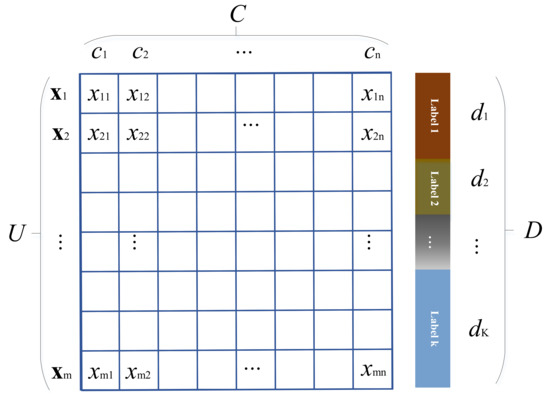
(Decision system) A binary group:can describe a decision system. Among them,is called the universe, which is a finite and nonempty set.is the set of decision attributes which is a nonempty set.is the collection of conditional attributes,,31. Therefore, the relationship between each element in a decision system can be represented as shown in Figure 1. To better understand the above definition, we describe the above-mentioned elements in combination with the fault diagnosis problem. C represents the parameters output by the sensor or the extracted feature attributes, D represents the category of the failure mode, and U denotes the collected data.
Figure 1.
The illustration of a decision system.
The decision-theoretic rough set (DTRS) presented by Yao et al. [33]. provides a concise semantic interpretation through a loss function matrix. The loss function matrix is described in Table 1.

Table 1.
The detailed information of a loss function matrix.
Consider that is the subset of samples with the same label . The state suggests that a related sample defined as is in , and the state suggests that is not in . The set of actions , , and indicate the classification of x into three regions, which are , , . denotes the acceptance of the event . denotes the deferment of the event , also considers denotes the non-commitment of the event . denotes the rejection of . Furthermore, denotes the loss caused by taking actions (, , ) while . is the loss caused by taking actions (, , ) while .
Consider this scenario: the risk of delaying the execution of the correct action is increased compared to that of the correct action, and both are less than the loss of taking the wrong action, the DTRS model therefore made a reasonable assumption: and , which is the basis for generating this rough set model.
Thanks to the above assumption, a pair of threshold parameters is used to define the positive region , the boundary region and the negative region to construct the DTRS model, which is guided by the Bayesian risk minimization principle and the three-way decision theory. Thus, we have the form of a DTRS model as follows 31:
The following equations represent the relationship between the two threshold parameters and the six loss functions:
The key parts of the DTRS model are the loss function or threshold parameter . To study and employ the DTRS model, an important issue is how to determine these parameters. Inspired by the idea of being data-driven, our previous work proposed a single-parameter decision-theoretic rough set (SPDTRS) model [32] that simplifies the traditional DTRS model. Specifically, the model requires only one parameter to be preset rather than the pair of or the six parameters in the loss function matrix. However, the solution of employing two truncation functions utilized in the model calculation makes the model relatively complex. Moreover, the interpretability of the loss function matrix in the SPDTRS model is slightly insufficient. The above two disadvantages are the focus of this paper in proposing a new rough set model.
3. Fuzzy Neighborhood ζ-Decision-Theoretic Rough Set
3.1. Granular Computing Based on Fuzzy Neighborhood Relationship
In order to be more applicable to practical problems, rough set models need to be able to handle a hybrid dataset, including continuous and discrete data. Fuzzy relationship and neighborhood relationship are two effective means to deal with the spatial relationship of samples. Their combined form is used by a variety of models [34]. The fuzzy neighborhood relationship can analyze the relationship between the entities in the decision system more precisely. Therefore, to overcome the inability of the SPDTRS model to handle the hybrid dataset, we introduce this fuzzy neighborhood relationship.
Definition 2.
(Fuzzy neighborhood relationship) Given a decision system, for an arbitrary sample, the fuzzy neighborhood subset of is defined as:
where is fuzzy neighborhood radius. The range of is . If and y are continuous data, we have . While the two elements and y are discrete data, we have
Thus, the fuzzy neighborhood subset is also called equivalence class. On this basis, the fuzzy conditional probability of could be described as:
where is the subset of samples with the same label . Under the assumption of the fuzzy neighborhood subset , we have , while if and only if . represents the sum of all elements in its set.
3.2. Determination of the Two Threshold Parameters
Considering the disadvantage of the SPDTRS model, a new loss function matrix is proposed, which is under fuzzy neighborhood relationship by a concise loss function relationship to avoid introducing the truncation functions. The novel SPDTRS model avoids the discussion of multiple situations and reduces the computational complexity of the SPDTRS model.
In the new loss function matrix, the data-driven loss functions under fuzzy neighborhood relationship is shown in Table 2. Besides, is the fuzzy neighborhood conditional probability, which can be calculated by Equation (8). The compensation coefficient is ζ with . and are the significance coefficients, which can be described as follows:
where represents the sum of all elements in its set.
Table 2.
The fuzzy neighborhood data-driven loss function matrix.
Under the assumption of the equivalence class , the relationships and hold, and if and only if .
Subsequently, we can conclude the pair of threshold parameters according to the fuzzy neighborhood data-driven loss function matrix, which can be represented as follows. In addition, we rewrite ,, for the sake of convenience.
Subsequently, we can set up three-way decision rules as follows:
Rule (P): Decide while ;
Rule (B): Decide while ;
Rule (N): Decide while .
According to the decision rules, the following roots about and can be described in the following two cases.
Case 1:
From the rule (P), we can obtain
From the rule (N), we can obtain
From these results, we can only accept two roots because of the relationship . Thus, we can rewrite these two roots:
Case 2:
The values of these two parameters are as follows:
The model arising from this case corresponds to the Pawlak model. Both boundary loss functions are equal to 0. Therefore the model clearly exhibits a two-way decision-making characteristic. Thus, the Pawlak model is one of the specific examples of our model, and is a necessary non-sufficient condition for it.
Theorem 1.
For the fuzzy neighborhood data-driven loss function matrix, assuming the equivalence class, whenholds, namely, the concerned equivalence class is not a consistent class, then we have:
(a1) ,
(a2) .
Whenholds, i.e., the concerned equivalence class is a consistent class, then we have:
(b1)
(b2)
Proof.
(a1) If , then , . Since , , then . Due to and , hence .
(a2) If , then , . Since , , then . Due to and , hence .
(b1) If , then , . Since , , then . Due to and , hence .
(b2) If , then , and . Since , , then . Due to and , hence . QED. □
3.3. Establishment of FNζDTRS
Reasoning by Section 3.2, the expressions of these two threshold functions lead to the following results: and under the above two conditions, where and . Based on Equations (9) and (10), it is easily to obtain and by confirming the parameter and analyzing the distribution information of the original data. In summary, we can change these two threshold parameters to , . The rough set model below, which is including parameters and is defined as fuzzy neighborhood ζ-decision-theoretic rough set (FNζDTRS):
where both threshold parameters have different descriptions under the following two conditions:
Case 1:
, then
Case 2:
, then
In the above FNζDTRS model, there are only two cases to discuss, in contrast to the SPDTRS model that requires four cases to discuss, which greatly reduces the computational complexity of the SPDTRS model due to the concise setting of loss functions.
Theorem 2.
In the FNζDTRS model, given two compensation coefficientsandwithand, and the parameteris fixed, if there exists, thenandhold.
Proof.
If the equivalence class , then , according to Equations (22)–(25), when , , , when , , . If the equivalence class , then its monotonicity relations will be proved by the following derivations.
Part I: For , two cases need to be considered.
Case 1:
Since , we set , due to , then and . Due to , , we can set for simplicity of derivation. We can find the partial derivative of it, denoted as , which is
Its second-order partial derivative is denoted as :
Because is less than 0, is monotonically decreasing. Since , , , then . Therefore, grows monotonically with respect to . Hence, decreases monotonically with respect to , that is .
Case 2:
In this case, we have . Thus, for , we have .
Part II: For , two cases need to be considered as well.
Case 1:
Since , we also set , due to , then and . Due to , , we have the simple form . We describe partial derivatives of like:
From , we know that increases monotonously along with . Since , , , then , and is monotonously decreasing with regard to . Therefore, is monotonously increasing with , that is . QED. □
Theorem 3.
In the FNζDTRS model, the relationshipholds.
Proof.
If the equivalence class , then , according to Equations (22)–(25), when , , when , , , satisfying the inequality . If the equivalence class , then in following three parts we intend to prove the inequality.
Part I: Proof of under two cases.
Case 1:
According to Equation (23), we could get , and then we only need to prove . Since , , then , so .
Case 2:
In this case, we have .
Part II: Proof of the inequality in two cases.
Case 1:
According to Equations (22) and (23), we could get
Since , , then
so , that is .
Case 2:
In this case, we have , , so .
Part III: Proof of the inequality in two cases.
Case 1:
According to Equation (22), if we want to prove , then we need to prove , which means we need to prove . Since , , then
Therefore, we have .
Case 2:
In this case, we have . QED. □
Theorem 4.
For a decision system, which is described aswith a fixed parameter, and two parametersandwith, we have,,.
Proof.
At the very beginning of the proof, we assume an arbitrary sample to facilitate the proof of the theorem. While , we have . Since , the relation holds according to Theorem 2. Thus, and hold. Hence, we conclude that .
Likewise, to conclude that and is easy via Theorem 2.
From the above, we can find that is inversely correlated with the range of neutrality and positively correlated with the uncertainty of the decision. QED. □
3.4. FNζDTRS-Based Attribute Reduction Algorithm
Jia et al. [35] presented a reduction principle in response to the problem of attribute reduction by using the DTRS model. The core idea of it is minimizing the risk of the reduction subset. On this principle, our previous work has designed an attribute reduction algorithm based on the SPDTRS model [32,34]. It is built on minimizing the risk of overall decisions, which can be utilized for the attribute reduction in our proposed FNζDTRS model. Therefore, the detailed attribute reduction algorithm is not repeated in this paper. For details, the readers could refer to our previous work [32,34].
4. Strategy of Simultaneous-Fault Diagnosis
Under the assumption that the data in all single-fault modes are fully available, when an unknown fault occurs, we use the FNζDTRS model to mine the fault attributes of the unknown fault. If the fault attributes of the unknown fault are different from the fault attributes of the existing single-fault, then the unknown fault can be considered as a simultaneous-fault. Furthermore, we can use the attribute reduction results obtained from the FNζDTRS model to analyze and identify the corresponding fault modes of the simultaneous-fault. Finally, a strategy of simultaneous-fault diagnosis called fault matching strategy is formed, as shown in Figure 2.
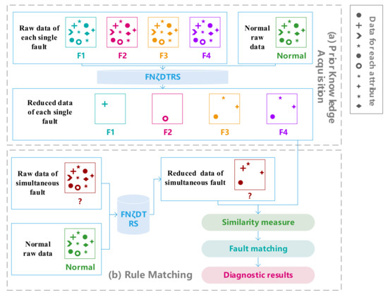
Figure 2.
The procedure of fault diagnosis strategy for simultaneous-fault.
The proposed fault matching strategy consists of two main parts, prior knowledge acquisition and rule matching. In the first part, the single-fault data with abnormal labels and normal data with normal labels are sent into the FNζDTRS model as the training data set, and the optimal fault attribute subsets of each single-fault are obtained by attribute reduction, used as the prior knowledge for subsequent diagnosis. In the second part, the simultaneous-fault data with abnormal labels and normal data with normal labels are combined to form the data to be diagnosed, and then the data are fed into the FNζDTRS model to obtain the optimal fault attribute subset. The optimal fault attribute subset is then obtained here and the optimal fault attribute subsets obtained in the first part are measured by using the Jaccard similarity coeffective. It is worth noting that there may be some single faults with the same fault attributes, therefore we set some rules based on the differences between attribute data to subdivide the faults and complete the fault matching, which can be seen in the subsequent experiments based on the satellite power system.
Based on the above description, we can write the core pseudo code in the above process, as shown in Table 3.
Table 3.
The core pseudo code of the diagnosis strategy.
5. Numerical Experiment of Attribute Reduction
The effectiveness and advantage of the proposed FNζDTRS model is verified on several hybrid decision systems from the UCI (http://archive.ics.uci.edu/ml/index.php, accessed on 21 July 2021) and KEEL (https://sci2s.ugr.es/keel/datasets.php, accessed on 21 July 2021) datasets. As shown in Table 4, the test datasets include both discrete and continuous data. Specific comparative experiments regarding parameters test and attribute reduction are conducted on the same hard and soft platforms. Ten baseline classifiers, including NaiveBayes, REPTree, LogitBoost, SMO, Filtered, Bagging, PART, IBk, J48 and JRip, are employed with a 10-fold cross-validation in Weka (https://waikato.github.io/weka-wiki/downloading_weka/, accessed on 21 July 2021) software to demonstrate the accuracy of attribute selection. The input data are normalized into the range of [0, 1] during preprocessing.
Table 4.
The information of the employed datasets.
5.1. Parameters Test for FNζDTRS
For the FNζDTRS model, two parameters and need to be set in advance. As described in Section 2, the theoretic value field of is , and is . Therefore, is sampled with an interval of 0.05, and end at 0.99. is also sampled with an interval of 0.05, but end at 1. Figure 3 shows the experimental results.
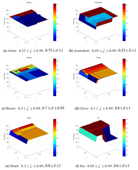
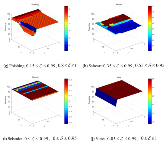
Figure 3.
The accuracy results of and with respect to FNζDTRS.
The results show that the appropriate settings of and range in [0.3, 0.99] and [0.85, 0.95], respectively. It could be explained by the fact that a smaller will result in a larger boundary region, marking more samples as uncertain state. It means setting a smaller for the FNζDTRS decision system will lead to greater uncertainty. When applied in real world, should be adjusted appropriately according to the risk of wrong decision. When the danger of making a bad decision is low, can be set larger, and vice versa. On the other hand, with the fuzzy neighborhood threshold closer to 1, the fuzzy neighborhood granules will be finer, allowing for the samples to be classified accurately into the appropriate regions. The above two parameters are the core parameters of the model proposed in this paper, and their setting values directly affect the test results. Therefore, when setting the above parameters, the values of the two parameters need to be adjusted according to the actual needs with the above principles.
5.2. Comparison Experiments on Attribute Reduction
In this part, seven related models, DTRS-EF [36], DTRS-SMDNS [37], SPDTRS-EF [32], SPDTRS-SMDNS [32], NDTRS [38], FDTRS [39] and FN3WD [34], are introduced into a contrastive analysis on the attribute reduction to demonstrate the superiority of the proposed FNζDTRS. The settings of the relevant parameters in these comparison models are the same as those of the corresponding models. The number of reduction attributes and the classification accuracy are the common evaluation indicators of the comparison experiment of attribute reduction [40,41]. The standard deviations of ten trials are also calculated, and the results are shown in Table 5 and Table 6.
Table 5.
The classification accuracy of the reduction subset.
Table 6.
The number of reduction attributes.
- (a)
- The analysis based on the classification accuracy indicates that the FNζDTRS model is superior to other rough set models. The main reason may lie in the different methods to describe spatial granules. Discretization methods such as EF and SMDNS are commonly introduced to process continuous data in the traditional DTRS models, which results in the destruction of the spatial structure of granules. Using special measures (such as fuzzy relationship, neighborhood relationship, etc.) can avoid the distortion of the discretization method, but it also has some disadvantages, such as simple measurement, insufficient description ability, etc. The proposed FNζDTRS model utilizes fuzzy neighborhood relationships to overcome the above shortcomings. Compared with other DTRS models, the description of spatial granules is more precise in our model and results in the higher classification accuracy.
- (b)
- With respect to the number of reduction attributes, the FDTRS model has the least number of reduction attributes, but it fails to achieve a desired classification accuracy, whereas the FNζDTRS model can maintain high classification accuracy while keeping the number of reduction attributes small. The results show that the classification ability can be maintained or improved only when the reduction attributes are accurately selected. The above conclusion also conforms to the basic principle of attribute reduction, that is, in the operation of reduction, we want to get a relatively concise set, which can ensure that the original classification accuracy is not reduced, and the purpose is to improve the operation efficiency.
- (c)
- The standard deviation is used to measure the robustness of models. It is obvious that the standard deviation of the FNζDTRS model is the smallest regardless of the classification accuracy or the number of reduced attributes, which directly proves that the robustness of the FNζDTRS model is the highest compared to other models. The above robustness characteristics also show that we have a large selection range when setting our two parameters, which is conducive to the wide application of the model in practical projects.
6. Simultaneous-Fault Diagnosis of Satellite Power System
In-orbit faults of the power system should be avoided to the maximum extent for satellites. Therefore, simulation is the best platform to mine fault diagnosis knowledge. In this section, the effectiveness of the proposed simultaneous-fault diagnosis scheme is verified with the simulation model of a geosynchronous (GEO) satellite power system [3]. As shown in Figure 4, the power system works in a direct energy transfer mode during the simulation, and ten telemetry parameters can be measured in the marked position. The information of the telemetry parameters is shown in Table 7.
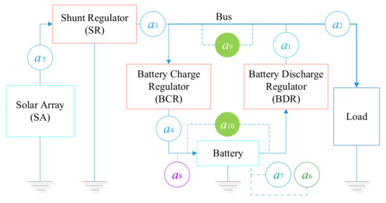
Figure 4.
The schematic diagram of the power system.
Table 7.
Information of the telemetry parameters.
The raw data used for simultaneous-fault diagnosis is composed of the above-mentioned ten kinds of attributes, and all the data are selected in the stationary period. The dataset is stored in a time-series format, with each subset representing one of the scenarios shown in Table 8. There are a total of 12 scenarios, where scenario 0 represents the system without any fault. F1 represents open-circuit failure in solar array. F2 represents the short-circuit failure in the battery. F3 represents shunt regulator failure without shunt. F4 represents shunt regulator failure with constant shunt. The remaining 7 scenarios are concurrent failures composed of the above 4 single failures occurring at the same time, where F3 and F4 cannot occur simultaneously.
Table 8.
Different scenarios for faults in satellite power system.
It can be seen that this means can effectively solve the problem of insufficient data in the simultaneous-fault diagnosis, which also responds to one the difficulties in the simultaneous-fault diagnosis introduced at the beginning of this paper.
6.1. Simultaneous-Fault Diagnosis Based on the Fault Matching Strategy
The two main parts of the simultaneous-fault diagnosis strategy, namely prior knowledge acquisition and rule matching, are equivalent to the training and testing process. We choose 4 kinds of single-fault data as the training set and the remaining 7 kinds of simultaneous-fault data as the testing set. The results obtained through the first step of prior knowledge acquisition are shown in Table 9. It can be found that the results of the output attribute subset of F3 and F4 are the same. Therefore, in order to distinguish F3 and F4, further information needs to be excavated. For attribute a3, its corresponding shunt current data can directly distinguish F3 from F4. The shunt current value of F3 fluctuates between 6.42–8.67 and that of F4 is between 12.45–14.77. Therefore, F3 and F4 can be distinguished by setting the threshold value of the shunt current average.
Table 9.
The results of the training process.
The results obtained through the second step of rule matching are shown in Table 10. For a simultaneous-fault, the Jaccard similarity coefficient between its output attribute subset and the output attribute subset of each single-fault obtained in the training process can be calculated in turn. If the Jaccard similarity coefficient is 0, the corresponding single fault can be eliminated preliminarily. Since F3 and F4 cannot be distinguished by the Jaccard similarity coefficient, it is necessary to further distinguish F3 and F4 through the set shunt current threshold and to finally obtain the matching result. Through the final matching result, it can be found that the diagnostic accuracy of the fault matching strategy is 100%. The above fault matching process comprehensively utilizes the similarity of attributes and expert knowledge, which can ensure that the obtained diagnosis results are more accurate.
Table 10.
The results of the testing process.
6.2. Comparison Experiment on Simultaneous-Fault Diagnosis
6.2.1. Experimental Setup
The superiority of the proposed fault matching strategy is demonstrated through comparison experiments of simultaneous-fault diagnosis with several multi-label classification algorithms (Binary Relevance, Classifier Chain, Calibrated Label Ranking, ML-KNN, and ML-DT). In these comparison algorithms, the classifiers of the first three algorithms are all set to Random Forest, which is the best classifier after the pretest, and the value of k for ML-KNN is 12. Subset accuracy, hamming loss, precision, recall, and F1 are introduced as the metrics of the multi-label classification performance [11].
The training set of all algorithms uses single-fault data, while the test set uses simultaneous-fault data. Ten-fold cross validation is also employed in this part.
6.2.2. Experimental Results and Analysis
The results are shown in Table 11. It is obvious that the proposed method outperforms other methods in the simultaneous-faults diagnosis of a satellite power system, which benefits from both the FNζDTRS model and the fault matching strategy (FNζDTRS-FMS). Fundamentally, on the one hand, the attribute reduction results obtained from the FNζDTRS model can accurately represent the fault information, and on the other hand, the proposed matching rules are reasonable and reliable.
Table 11.
The results of the simultaneous-fault diagnosis.
In addition to the results of our method, as for multi-label classification methods, the false alarm rate performs satisfactorily, while the missed diagnosis rate performs poorly. It can be seen that the recall rates have been lower than 50%, which is unacceptable in engineering applications. At the same time, the results of the F1 index generated by the multi-label classification methods are relatively low, only slightly higher than 60%. Similarly, the results obtained by the Calibrated Label Ranking method are similar to those of ML-KNN and ML-DT. The results obtained by the Classifier Chain method are in the middle level. In addition, Binary Relevance has the best performance among the multi-label classification methods, which means that there are no relevant dependencies between the single faults.
7. Conclusions
In this work, a novel DTRS model called FNζDTRS is proposed and the fault match strategy (FMS) based on the FNζDTRS model is designed to overcome three fundamental hurdles faced by simultaneous-fault diagnosis. The effectiveness and superiority of our methodology is demonstrated by both numerical experiments conducted on several standard datasets and comparison analysis of simultaneous-fault diagnosis performed on a simulation model of a satellite power system. Consequently, two main conclusions can be drawn, as follows.
- (1)
- The proposed FNζDTRS model performs attribute reduction more effectively compared with other models, and it has strong generalization ability. This benefits from the concise loss functions and the introduction of the fuzzy neighborhood relationships. The advantages of our model can greatly promote the smooth implementation of the model in simultaneous-fault diagnosis, which reflects the effectiveness and superiority of our selection of this model.
- (2)
- The proposed FNζDTRS–FMS does not require simultaneous-fault samples to accomplish training and performs excellently in simultaneous-fault diagnosis compared to classic multi-label classification algorithms. This is completely consistent with the real situation, that is, the existing data cannot completely cover all the imagined failure modes. Therefore, the diagnostic strategy proposed in this paper has stronger application value.
Although the model we proposed has the above advantages, it still has the problem of low computational efficiency compared with the classical rough set because of the use of fuzzy neighborhood computing. This is one of our future research directions. Furthermore, our future work will also focus on fusing rough set models and multi-label learning algorithms to make the simultaneous-fault diagnosis framework more general.
Author Contributions
Data curation, R.Z.; Formal analysis, Y.J. and T.Z.; Funding acquisition, C.L. and M.S.; Methodology, L.T. and C.W.; Writing—original draft, Y.C., Y.J. and M.S.; Validation, Y.J.; Investigation, T.Z.; Supervision, M.S. All authors have read and agreed to the published version of the manuscript.
Funding
This study was supported by the National Natural Science Foundation of China (Grant Nos. 61903015 and 61973011), the Fundamental Research Funds for the Central Universities (Grant No. KG21003001), National key Laboratory of Science and Technology on Reliability and Environmental Engineering (Grant No. WDZC2019601A304), as well as the Capital Science & Technology Leading Talent Program (Grant No. Z191100006119029).
Data Availability Statement
The public data can be accessed through the following two websits: the UCI (http://archive.ics.uci.edu/ml/index.php, accessed on 21 July 2021) and KEEL (https://sci2s.ugr.es/keel/datasets.php, accessed on 21 July 2021). However, the data set of the satellite power system is not convenient for public display. If necessary, researchers can make further consultation via email.
Acknowledgments
Thank the reviewers for their comments on improving the quality of our papers, and thank the journal editors for their enthusiastic work.
Conflicts of Interest
The authors declare no conflict of interest.
Nomenclature
| the universe, which is a finite and nonempty set. | |
| the set of decision attributes that is a nonempty set. | |
| the collection of conditional attributes. | |
| the subset of samples with the same label . | |
| , , and | the classification of x into three regions, which are , , . |
| the acceptance of the event . | |
| the non-commitment of the event , denotes the deferment of the event . | |
| the rejection of . | |
| the loss caused by taking actions (, , ) while . | |
| the loss caused by taking actions (, , ) while . | |
| the threshold parameters of the DTRS model. | |
| fuzzy neighborhood radius. | |
| the compensation coefficient. |
References
- Li, S.; Cao, H.; Yang, Y. Data-driven simultaneous fault diagnosis for solid oxide fuel cell system using multi-label pattern identification. J. Power Sources 2018, 378, 646–659. [Google Scholar] [CrossRef]
- Suo, M.; Tao, L.; Zhu, B.; Chen, Y.; Lu, C.; Ding, Y. Soft decision-making based on decision-theoretic rough set and Takagi-Sugeno fuzzy model with application to the autonomous fault diagnosis of satellite power system. Aerosp Sci. Technol. 2020, 106, 106108. [Google Scholar] [CrossRef]
- Suo, M.; Zhu, B.; An, R.; Sun, H.; Xu, S.; Yu, Z. Data-driven fault diagnosis of satellite power system using fuzzy Bayes risk and SVM. Aerosp Sci. Technol. 2019, 84, 1092–1105. [Google Scholar] [CrossRef]
- Asgari, S.; Gupta, R.; Puri, I.K.; Zheng, R. A data-driven approach to simultaneous fault detection and diagnosis in data centers. Appl. Soft Comput. 2021, 110, 107638. [Google Scholar] [CrossRef]
- Liang, P.; Deng, C.; Wu, J.; Yang, Z.; Zhu, J.; Zhang, Z. Single and simultaneous fault diagnosis of gearbox via a semi-supervised and high-accuracy adversarial learning framework. Knowl.-Based Syst. 2020, 198, 105895. [Google Scholar] [CrossRef]
- Zhang, Z.; Li, S.; Xiao, Y.; Yang, Y. Intelligent simultaneous fault diagnosis for solid oxide fuel cell system based on deep learning. Appl. Energ. 2019, 233, 930–942. [Google Scholar] [CrossRef]
- Pooyan, N.; Shahbazian, M.; Salahshoor, K.; Hadian, M. Simultaneous Fault Diagnosis using multi class support vector machine in a Dew Point process. J. Nat. Gas. Sci. Eng. 2015, 23, 373–379. [Google Scholar] [CrossRef]
- Vong, C.; Wong, P.; Ip, W. A New Framework of Simultaneous-Fault Diagnosis Using Pairwise Probabilistic Multi-Label Classification for Time-Dependent Patterns. Ieee T Ind. Electron. 2013, 60, 3372–3385. [Google Scholar] [CrossRef]
- Wong, P.K.; Zhong, J.; Yang, Z.; Vong, C.M. Sparse Bayesian extreme learning committee machine for engine simultaneous fault diagnosis. Neurocomputing 2016, 174, 331–343. [Google Scholar] [CrossRef]
- Wu, B.; Cai, W.; Chen, H.; Zhang, X. A hybrid data-driven simultaneous fault diagnosis model for air handling units. Energy Build. 2021, 245, 111069. [Google Scholar] [CrossRef]
- Zhang, M.; Zhou, Z. A Review on Multi-Label Learning Algorithms. IEEE Trans. Knowl. Data Eng. 2014, 26, 1819–1837. [Google Scholar] [CrossRef]
- Boutell, M.R.; Luo, J.B.; Shen, X.P.; Brown, C.M. Learning multi-label scene classification. Pattern Recognit. 2004, 37, 1757–1771. [Google Scholar] [CrossRef]
- Read, J.; Pfahringer, B.; Holmes, G.; Frank, E. Classifier chains for multi-label classification. Mach. Learn. 2011, 85, 333–359. [Google Scholar] [CrossRef]
- Fuernkranz, J.; Huellermeier, E.; Mencia, E.L.; Brinker, K. Multilabel classification via calibrated label ranking. Mach. Learn. 2008, 73, 133–153. [Google Scholar] [CrossRef]
- Zhang, M.; Zhou, Z. ML-KNN: A lazy learning approach to multi-label leaming. Pattern Recognit. 2007, 40, 2038–2048. [Google Scholar] [CrossRef]
- Clare, A.; King, R.D. Knowledge Discovery in Multi-label Phenotype Data. In European Conference on Principles of Data Mining and Knowledge Discovery; Springer: Berlin/Heidelberg, Germany, 2001; pp. 42–53. [Google Scholar]
- Pawlak, Z. Rough sets. Int. J. Comput. Inf. Sci. 1982, 11, 341–356. [Google Scholar] [CrossRef]
- Dong, L.; Chen, D.; Wang, N.; Lu, Z. Key energy-consumption feature selection of thermal power systems based on robust attribute reduction with rough sets. Inf. Sci. 2020, 532, 61–71. [Google Scholar] [CrossRef]
- Su, L.; Yu, F. Matrix approach to spanning matroids of rough sets and its application to attribute reduction. Theor. Comput. Sci. 2021, 893, 105–116. [Google Scholar] [CrossRef]
- Sahu, R.; Dash, S.R.; Das, S. Career selection of students using hybridized distance measure based on picture fuzzy set and rough set theory. Decis. Mak. Appl. Manag. Eng. 2021, 4, 104–126. [Google Scholar] [CrossRef]
- Dash, S.R.; Dehuri, S.; Sahoo, U.K. Interactions and Applications of Fuzzy, Rough, and Soft Set in Data Mining. Int. J. Fuzzy Syst. Appl. 2015, 3, 37–50. [Google Scholar] [CrossRef]
- Zhang, P.; Li, T.; Wang, G.; Luo, C.; Chen, H.; Zhang, J.; Wang, D.; Yu, Z. Multi-source information fusion based on rough set theory: A review. Inf. Fusion 2021, 68, 85–117. [Google Scholar] [CrossRef]
- Bai, H.; Ge, Y.; Wang, J.; Li, D.; Liao, Y.; Zheng, X. A method for extracting rules from spatial data based on rough fuzzy sets. Knowl.-Based Syst. 2014, 57, 28–40. [Google Scholar] [CrossRef]
- Landowski, M.; Landowska, A. Usage of the rough set theory for generating decision rules of number of traffic vehicles. Transp. Res. Procedia 2019, 39, 260–269. [Google Scholar] [CrossRef]
- Sharma, H.K.; Kumari, K.; Kar, S. A rough set theory application in forecasting models. Decis. Mak. Appl. Manag. Eng. 2020, 3, 1–21. [Google Scholar] [CrossRef]
- Guo, Y.; Tsang, E.C.C.; Xu, W.; Chen, D. Adaptive weighted generalized multi-granulation interval-valued decision-theoretic rough sets. Knowl.-Based Syst. 2020, 187, 104804. [Google Scholar] [CrossRef]
- Wang, T.; Liu, W.; Zhao, J.; Guo, X.; Terzija, V. A rough set-based bio-inspired fault diagnosis method for electrical substations. Int. J. Electr. Power Energy Syst. 2020, 119, 105961. [Google Scholar] [CrossRef]
- Sang, B.; Yang, L.; Chen, H.; Xu, W.; Guo, Y.; Yuan, Z. Generalized multi-granulation double-quantitative decision-theoretic rough set of multi-source information system. Int. J. Approx. Reason. 2019, 115, 157–179. [Google Scholar] [CrossRef]
- Zhang, P.F.; Li, T.R.; Yuan, Z.; Luo, C.; Liu, K.Y.; Yang, X.L. Heterogeneous Feature Selection Based on Neighborhood Combination Entropy. IEEE Trans. Neural Netw. Learn. Syst. 2022, 1–14. [Google Scholar] [CrossRef]
- Wang, L.; Shen, J.; Mei, X. Cost Sensitive Multi-Class Fuzzy Decision-theoretic Rough Set Based Fault Diagnosis. In Proceedings of the 2017 36th Chinese Control Conference (CCC), Dalian, China, 26–28 July 2017; pp. 6957–6961. [Google Scholar]
- Yu, J.; Ding, B.; He, Y. Rolling bearing fault diagnosis based on mean multigranulation decision-theoretic rough set and non-naive Bayesian classifier. J. Mech. Sci. Technol. 2018, 32, 5201–5211. [Google Scholar] [CrossRef]
- Suo, M.; Tao, L.; Zhu, B.; Miao, X.; Liang, Z.; Ding, Y.; Zhang, X.; Zhang, T. Single-parameter decision-theoretic rough set. Inf. Sci. 2020, 539, 49–80. [Google Scholar] [CrossRef]
- Yao, Y.Y.; Wong, S.K.M. A decision theoretic framework for approximating concepts. Int. J. Man Mach. Stud. 1992, 37, 793–809. [Google Scholar] [CrossRef]
- Suo, M.; Cheng, Y.; Zhuang, C.; Ding, Y.; Lu, C.; Tao, L. Extension of labeled multiple attribute decision making based on fuzzy neighborhood three-way decision. Neural Comput. Appl. 2020, 32, 17731–17758. [Google Scholar] [CrossRef]
- Jia, X.; Liao, W.; Tang, Z.; Shang, L. Minimum cost attribute reduction in decision-theoretic rough set models. Inf. Sci. 2013, 219, 151–167. [Google Scholar] [CrossRef]
- Yao, Y. Three-way decisions with probabilistic rough sets. Inf. Sci. 2010, 180, 341–353. [Google Scholar] [CrossRef]
- Jiang, F.; Sui, Y. A novel approach for discretization of continuous attributes in rough set theory. Knowl.-Based Syst. 2015, 73, 324–334. [Google Scholar] [CrossRef]
- Li, W.; Huang, Z.; Jia, X.; Cai, X. Neighborhood based decision-theoretic rough set models. Int. J. Approx. Reason. 2016, 69, 1–17. [Google Scholar] [CrossRef]
- Song, J.; Tsang, E.C.C.; Chen, D.; Yang, X. Minimal decision cost reduct in fuzzy decision-theoretic rough set model. Knowl.-Based Syst. 2017, 126, 104–112. [Google Scholar] [CrossRef]
- Wang, C.; Qi, Y.; Shao, M.; Hu, Q.; Chen, D.; Qian, Y.; Lin, Y. A Fitting Model for Feature Selection with Fuzzy Rough Sets. IEEE Trans. Fuzzy Syst. 2017, 25, 741–753. [Google Scholar] [CrossRef]
- Wang, C.; Shao, M.; He, Q.; Qian, Y.; Qi, Y. Feature subset selection based on fuzzy neighborhood rough sets. Knowl.-Based Syst. 2016, 111, 173–179. [Google Scholar] [CrossRef]
Publisher’s Note: MDPI stays neutral with regard to jurisdictional claims in published maps and institutional affiliations. |
© 2022 by the authors. Licensee MDPI, Basel, Switzerland. This article is an open access article distributed under the terms and conditions of the Creative Commons Attribution (CC BY) license (https://creativecommons.org/licenses/by/4.0/).