A Time-Inhomogeneous Prendiville Model with Failures and Repairs

Abstract

We consider a time-inhomogeneous Markov chain with a finite state-space which models a system in which failures and repairs can occur at random time instants. The system starts from any state j (operating, F, R). Due to a failure, a transition from an operating state to F occurs after which a repair is required, so that a transition leads to the state R. Subsequently, there is a restore phase, after which the system restarts from one of the operating states. In particular, we assume that the intensity functions of failures, repairs and restores are proportional and that the birth-death process that models the system is a time-inhomogeneous Prendiville process.

1. Introduction

Continuous-time Markov chains (CTMC) are usually used in various application fields related to queueing systems, mathematical biology, physics, and chemistry (cf., for instance, Anderson [1], Iosifescu and Tautu [2], Medhi [3], Bayley [4], van Kampen [5], Taylor and Karlin [6], Sericola [7]). In these cases, the stochastic process describes the evolution in continuous time of a Markov chain with a countable set of states that represent the number of customers in a queue, the number of molecules in a chemical reaction, the size of the population with births/deaths/immigrations/emigrations.

In the recent decades, particular attention has been paid to the study of these processes under the effect of random catastrophes that produce a sudden change of the state of a system. After such failure, one can think that the system is empty (total catastrophes) and then the dynamics immediately restart without delay (cf., for instance, Dharmaraja et al. [8], Giorno et al. [9,10,11], Di Crescenzo et al. [12], Economou and Fakinos [13,14], Chen et al. [15]). In more realistic cases, after a failure the system can be shipped for maintenance; in these cases, due to the extent of the failure, it is reasonable to assume random repair times. To introduce the effect of a catastrophe related to a failure of the system, one adds to the usual assumptions the existence of a non-zero probability of transition to an intermediate state from which the zero, or another operating state, can be reached at some randomly distributed instants (cf., for instance, Di Crescenzo et al. [16,17], Ye et al. [18], Mytalas and Zazanis [19], Krishna Kumar et al. [20]). In many cases, the times to failures and the times of repair are assumed to be exponential random variables. Some models consider the phase-type distributions for failure and repair times (see, for instance, Altiok [21,22,23], Dallery [24]).

Frequently, time-inhomogeneous Markov chains are used to model real dynamic systems. Research in this area are oriented to determine the transient and the limiting probability distribution, and to construct a continuous time diffusion approximation (cf., for instance, Kendall [25], McNeil and Schach [26], Di Crescenzo et al. [27,28], Giorno et. al. [29,30]). Moreover, some studies on the ergodicity of time-inhomogeneous birth-death chains are considered in Ammar et al. [31], Zeifman et al. [32,33], Satin et al. [34]. For CTMC, the evaluation of first-passage time densities and their moments via analytical and numerical methods plays an important role (cf., for instance, Jouini [35], Giorno and Nobile [36] and references therein).

Various research have been devoted to stochastic “logistic models” that describe biological population growth in a limited environment or the number of customers in a queueing system with finite capacity. In particular, the logistic model proposed by Prendiville in 1949, and subsequently solved by Takashima in 1956, was applied in biology, in ecology and in queueing systems (cf. Prendiville [37], Takashima [38], Giorno et al. [39], Ricciardi [40]). The Prendiville process can be also viewed as the Ehrenfest model in continuous time (see, Karlin and McGregor [41], Flegg et al. [42]). Furthermore, Zheng [43] gives the extension of the Prendiville process to the inhomogeneous case. The Prendiville/Ehrenfest model has been also used to describe queueing systems in presence of catastrophes (cf. Dharmaraja [8], Giorno [44,45]). Moreover, Parthasarathy and Krishna Kumar [46] and Matis and Kiffe [47] consider stochastic compartment models with Prendiville growth mechanisms.

In the present paper, we consider a time-inhomogeneous birth-death process with a finite state-space and we assume that failures and repairs can occur at random time instants. Specifically, the state-space of the considered stochastic process, in addition to the operating states, includes two particular states, denoted by F and R. The dynamics system starts from any state j (operating, F, R). Due to a failure that occurs according to a non-stationary exponential distribution, a transition from an operating state to F occurs; after which a repair, that leads to the state R, starting from F, is required. Even the repair times are assumed to be random and they occur according to a non-stationary exponential distribution. After the system has been repaired, it restarts from one of the operating states.

The plan of the paper is as follows. In Section 2, we describe the stochastic model; we provide the Kolmogorov differential equations for the time-inhomogeneous CTMC with a finite state-space, assuming that the times of failures, repairs, and restores are exponentially distributed. In Section 3, we assume that the failures, repairs and restores intensity functions are proportional; we determine the transient probabilities that, starting from an arbitrary state j at time $t_0$, the system reaches the state F, or the state R or one of the operating states $0,1,\dots ,\ell$ at time t. In Section 4, we analyze the time of first failure and determine its probability density function and related average. In Section 5, we obtain the probability generating function of the operating states of the system and the related conditional mean. In Section 6, the asymptotic behavior of the probabilities and of related average for the operating state is studied, under the assumption of proportional intensity functions.

2. The Model

Let $\{N\left(t\right),t\ge t_0\}$ be a time-inhomogeneous Markov chain with space-state $\mathcal{S}=\{-2,-1,0,1,\dots ,\ell \}$, where $n=-2$ corresponds to the failure state (F), $n=-1$ describes the repair state (R) from which the process can work again and $n=0,1,\dots ,\ell$ correspond to the operating states of the system (see, Figure 1). We assume that the arrival (upward jumps) and departures (downward jumps) at time t occur with intensity functions ${\lambda }_n\left(t\right)$ for $n=0,1,\dots ,\ell$ and ${\mu }_n\left(t\right)$ for $n=1,2,\dots ,\ell$, respectively. Moreover, the failures occur according to a non-homogeneous Poisson process, with intensity function ${\xi }_n\left(t\right)$, starting from the operating state n, with $n=0,1,\dots ,\ell$. If a failure occurs, then the system goes into the failure state F, and further, the completion of a repair occurs according to the intensity function $\varrho \left(t\right)$. After the repair, there is a restore phase after which the system restarts from an operating state n, with the intensity function ${\gamma }_n\left(t\right)$ for $n=0,1,\dots ,\ell$. Several cases can occur: (a) after the repair the system restarts from the state $n=0$, so that we have ${\gamma }_0\left(t\right)=\gamma \left(t\right)$ and ${\gamma }_n\left(t\right)=0$ for $n=1,2\dots ,\ell$; (b) the state from which the system restarts is chosen randomly, by setting ${\gamma }_n\left(t\right)=\gamma \left(t\right)$ for $n=0,1,2\dots ,\ell$; (c) the intensity functions ${\gamma }_0\left(t\right),{\gamma }_1\left(t\right),\dots ,{\gamma }_{\ell }\left(t\right)$ are chosen by reflecting the priority of one state over the others.

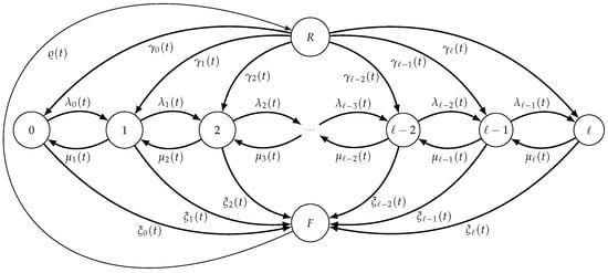
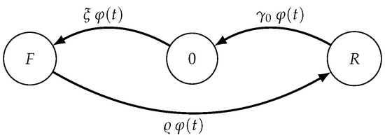
Figure 1. The state diagram of the Markov process $N\left(t\right)$ modeling failures and repairs.

Specifically, in any small interval $(t,t+\Delta t)$, $\Delta t>0$, we assume that the transitions that regulate $N\left(t\right)$ occur according the following scheme:

• $n\to n+1$ with intensity function ${\lambda }_n\left(t\right)$ for $n=0,1,\dots ,\ell -1$,
• $n\to n-1$ with intensity function ${\mu }_n\left(t\right)$ for $n=1,2,\dots ,\ell$,
• $-1\to n$ with intensity function ${\gamma }_n\left(t\right)$ for $n=0,1,\dots ,\ell$,
• $n\to -2$ with intensity function ${\xi }_n\left(t\right)$ for $n=0,1,\dots ,\ell$,
• $-2\to -1$ with intensity function $\varrho \left(t\right)$,

where ${\lambda }_n\left(t\right),{\mu }_n\left(t\right),{\gamma }_n\left(t\right),{\xi }_n\left(t\right),\varrho \left(t\right)$ are positive, bounded and continuous functions for $t\ge 0$. In Buonocore et al. [48], a time-homogeneous similar model is considered in the biological context, assuming that ${\lambda }_n\left(t\right)=\lambda$, for $n=0,1,\dots ,\ell -1$, ${\mu }_n\left(t\right)=\mu$, for $n=0,1,\dots ,\ell -1$, ${\gamma }_n\left(t\right)=\gamma$ for $n=0,1,\dots ,\ell$, ${\xi }_n\left(t\right)=\xi$ for $n=0,1,\dots ,\ell$ and $\varrho \left(t\right)=\varrho$.

Let

$$p_{j,n}\left(t\right|t_0)=P\{N\left(t\right)=n|N\left(t_0\right)=j\},j,n\in \mathcal{S}$$

(1)

be the transition probabilities of $N\left(t\right)$. Setting

$$\nu \left(t\right)=\sum _{n=0}^{\ell }{\gamma }_n\left(t\right),$$

(2)

one has:

$$\begin{array}{ccc}& & \frac{d{p}_{j,-2}\left(t\right|t_0)}{dt}=\sum _{n=0}^{\ell }{\xi }_n\left(t\right)p_{j,n}\left(t\right|t_0)-\varrho \left(t\right)p_{j,-2}\left(t\right|t_0)\hfill \\ & & \frac{d{p}_{j,-1}\left(t\right|t_0)}{dt}=-\nu \left(t\right)p_{j,-1}\left(t\right|t_0)+\varrho \left(t\right)p_{j,-2}\left(t\right|t_0),\hfill \\ & & \frac{d{p}_{j,0}\left(t\right|t_0)}{dt}={\gamma }_0\left(t\right)p_{j,-1}\left(t\right|t_0)-[{\lambda }_0\left(t\right)+{\xi }_0\left(t\right)]p_{j,0}\left(t\right|t_0)+{\mu }_1\left(t\right)p_{j,1}\left(t\right|t_0),\hfill \\ & & \frac{d{p}_{j,n}\left(t\right|t_0)}{dt}={\gamma }_n\left(t\right)p_{j,-1}\left(t\right|t_0)+{\lambda }_{n-1}\left(t\right)p_{j,n-1}\left(t\right|t_0)\hfill \\ & & -[{\lambda }_n\left(t\right)+{\mu }_n\left(t\right)+{\xi }_n\left(t\right)]p_{j,n}\left(t\right|t_0)+{\mu }_{n+1}\left(t\right)p_{j,n+1}\left(t\right|t_0),n=1,2,\dots ,\ell -1,\hfill \\ & & \frac{d{p}_{j,\ell }\left(t\right|t_0)}{dt}={\gamma }_{\ell }\left(t\right)p_{j,-1}\left(t\right|t_0)+{\lambda }_{\ell -1}\left(t\right)p_{j,\ell -1}\left(t\right|t_0)-[{\mu }_{\ell }\left(t\right)+{\xi }_{\ell }\left(t\right)]p_{j,\ell }\left(t\right|t_0),\hfill \end{array}$$

(3)

to solve with the initial conditions

$$\underset{t\downarrow t_0}{lim}{p}_{j,n}\left(t\right|t_0)={\delta }_{j,n}j,n\in \mathcal{S}.$$

(4)

For $t\ge t_0$ , denoting by

$${\mathcal{P}}_j\left(t\right|t_0)=\sum _{n=0}^{\ell }{p}_{j,n}\left(t\right|t_0),j\in \mathcal{S},$$

(5)

the probability that the system is in an operating state at time t, one has:

$${\mathcal{P}}_j\left(t\right|t_0)+p_{j,-2}\left(t\right|t_0)+p_{j,-1}\left(t\right|t_0)=1,j\in \mathcal{S}.$$

(6)

If ${\xi }_n\left(t\right)=\xi \left(t\right)$ for $n=0,1,\dots ,\ell$ and $t\ge t_0$, by virtue of (6), one obtains

$$\sum _{n=0}^{\ell }{\xi }_n\left(t\right)p_{j,n}\left(t\right|t_0)=\xi \left(t\right)[1-p_{j,-1}\left(t\right|t_0)-p_{j,-2}\left(t\right|t_0)],$$

so that the first two equations of system (3) become:

$$\begin{array}{cc}\hfill & \frac{d{p}_{j,-2}\left(t\right|t_0)}{dt}=\xi \left(t\right)[1-p_{j,-1}\left(t\right|t_0)]-[\xi \left(t\right)+\varrho \left(t\right)]p_{j,-2}\left(t\right|t_0),\hfill \\ \hfill & \frac{d{p}_{j,-1}\left(t\right|t_0)}{dt}=-\nu \left(t\right)p_{j,-1}\left(t\right|t_0)+\varrho \left(t\right)p_{j,-2}\left(t\right|t_0),\hfill \end{array}$$

(7)

to solve with the initial conditions

$$\underset{t\downarrow t_0}{lim}{p}_{j,-2}\left(t\right|t_0)={\delta }_{j,-2},\underset{t\downarrow t_0}{lim}{p}_{j,-1}\left(t\right|t_0)={\delta }_{j,-1}.$$

(8)

Furthermore, if ${\xi }_n\left(t\right)=\xi \left(t\right)$ for $n=0,1,\dots ,\ell$ and $t\ge t_0$, by virtue of (3), one has that the probability ${\mathcal{P}}_j\left(t\right|t_0)$ satisfies the following differential equation

$$\frac{d{\mathcal{P}}_j\left(t\right|t_0)}{dt}=-\xi \left(t\right){\mathcal{P}}_j\left(t\right|t_0)+\nu \left(t\right)p_{j,-1}\left(t\right|t_0)$$

(9)

to solve with the initial condition

$$\underset{t\downarrow t_0}{lim}{\mathcal{P}}_j\left(t\right|t_0)=1-{\delta }_{j,-2}-{\delta }_{j,-1}.$$

(10)

Equation (9) shows that the probability that the system is in an operating state at time t does not depend on the intensity functions ${\lambda }_n\left(t\right)$ and ${\mu }_n\left(t\right)$ related to the birth-death process without failures and repairs.

3. Proportional Intensity Functions of Failures, Repairs and Restores

We assume that

$$\begin{array}{cc}\hfill & \varrho \left(t\right)=\varrho \phi \left(t\right),{\xi }_n\left(t\right)=\xi \phi \left(t\right),{\gamma }_n\left(t\right)={\gamma }_n\phi \left(t\right),n=0,1,\dots ,\ell ,\hfill \\ \hfill & \nu \left(t\right)=({\gamma }_0+{\gamma }_1+\dots +{\gamma }_{\ell })\phi \left(t\right),\hfill \end{array}$$

(11)

where $\phi \left(t\right)$ is a positive, bounded and continuous function for $t\ge 0$. We denote by

$$\mathsf{\Phi }\left(t\right|t_0)={\int }_{t_0}^t\phi \left(u\right)du,t\ge t_0$$

(12)

and we assume that ${lim}_{t\to +\infty }\mathsf{\Phi }\left(t\right|t_0)=+\infty$.

3.1. Asymptotic Behavior of the System

Let

$$q_n=\underset{t\to +\infty }{lim}{p}_{j,n}\left(t\right|t_0),j,n\in \mathcal{S},Q=\sum _{n=0}^{\ell }{q}_n=1-q_{-2}-q_{-1},$$

(13)

be the steady-state probabilities of the considered system.

Proposition 1.

Under the assumptions (11), one has:

$$q_{-2}=\frac{\nu \xi }{\nu \varrho +\nu \xi +\varrho \xi },q_{-1}=\frac{\varrho \xi }{\nu \varrho +\nu \xi +\varrho \xi },Q=\frac{\varrho \nu }{\nu \varrho +\nu \xi +\varrho \xi }·$$

(14)

Proof. 

It follows from (7), by taking the limit as $t\to +\infty$. □

Note that the last identity in (14) is the probability that the system is in an operating state $n=0,1,\dots ,\ell$ in equilibrium regime.

3.2. Transient Behavior of the System

To determine the transient solution of system (7) with initial conditions (8), we denote by $x_1$ and $x_2$ the solutions of the following equation:

$$x^2+(\nu +\varrho +\xi )x+\nu \varrho +\nu \xi +\varrho \xi =0$$

and set

$$\Delta ={(\nu -\varrho -\xi )}^2-4\varrho \xi .$$

(15)

Since $x_1+x_2=-(\varrho +\xi +\nu )<0$ and $x_1{x}_2=\nu (\varrho +\xi )+\xi \varrho >0$, for $\Delta \ge 0$ one has that $x_1<0$ and $x_2<0$.

Proposition 2.

Under the assumptions (11), for $t\ge t_0$ the following results hold:

(i) 

If $\Delta >0$,

$$\begin{array}{ccc}& & p_{j,-2}\left(t\right|t_0)=q_{-2}+[{\delta }_{j,-2}-q_{-2}]Z_1\left(t\right|t_0)+[\xi (1-{\delta }_{j,-1})-(\xi +\varrho ){\delta }_{j,-2}]Z_2\left(t\right|t_0),\hfill \\ & & p_{j,-1}\left(t\right|t_0)=q_{-1}+[{\delta }_{j,-1}-q_{-1}]Z_1\left(t\right|t_0)+[-\nu {\delta }_{j,-1}+\varrho {\delta }_{j,-2}]Z_2\left(t\right|t_0),\hfill \\ & & {\mathcal{P}}_j\left(t\right|t_0)=Q+[1-Q-{\delta }_{j,-2}-{\delta }_{j,-1}]Z_1\left(t\right|t_0)+[(\xi +\nu ){\delta }_{j,-1}-\xi (1-{\delta }_{j,-2})]Z_2\left(t\right|t_0),\hfill \end{array}$$

with

$$Z_1\left(t\right|t_0)=\frac{x_1{e}^{x_2\mathsf{\Phi }\left(t\right|t_0)}-x_2{e}^{x_1\mathsf{\Phi }\left(t\right|t_0)}}{x_1-x_2},Z_2\left(t\right|t_0)=\frac{e^{x_1\mathsf{\Phi }\left(t\right|t_0)}-e^{x_2\mathsf{\Phi }\left(t\right|t_0)}}{x_1-x_2}.$$

(ii) 

If $\Delta =0$,

$$\begin{array}{ccc}& & p_{j,-2}\left(t\right|t_0)=q_{-2}+e^{x_1\mathsf{\Phi }\left(t\right|t_0)}\{{\delta }_{j,-2}-q_{-2}+\mathsf{\Phi }\left(t\right|t_0)[\xi (1-{\delta }_{j,-1})-(\xi +\varrho ){\delta }_{j,-2}\hfill \\ & & -x_1({\delta }_{j,-2}-q_{-2})\left]\right\},\hfill \\ & & p_{j,-1}\left(t\right|t_0)=q_{-1}+e^{x_1\mathsf{\Phi }\left(t\right|t_0)}\{{\delta }_{j,-1}-q_{-1}+\mathsf{\Phi }\left(t\right|t_0)[-\nu {\delta }_{j,-1}+\varrho {\delta }_{j,-2}\hfill \\ & & -x_1({\delta }_{j,-1}-q_{-1})\left]\right\},\hfill \\ & & {\mathcal{P}}_j\left(t\right|t_0)=Q+e^{x_1\mathsf{\Phi }\left(t\right|t_0)}\{1-Q-{\delta }_{j,-2}-{\delta }_{j,-1}+\mathsf{\Phi }\left(t\right|t_0)[(\xi +\nu ){\delta }_{j,-1}-\xi (1-{\delta }_{j,-2})\hfill \\ & & -x_1(1-Q-{\delta }_{j,-2}-{\delta }_{j,-1})\left]\right\},\hfill \end{array}$$

(iii) 

If $\Delta <0$,

$$\begin{array}{ccc}& & p_{j,-2}\left(t\right|t_0)=q_{-2}+e^{a\mathsf{\Phi }\left(t\right|t_0)}\{({\delta }_{j,-2}-q_{-2})cos\left[b\mathsf{\Phi }\left(t\right|t_0)\right]\hfill \\ & & +\frac{1}{b}[-a({\delta }_{j,-2}-q_{-2})-(\xi +\varrho ){\delta }_{j,-2}+\xi (1-{\delta }_{j,-1})]sin\left[b\mathsf{\Phi }\left(t\right|t_0)\right]\},\hfill \\ & & p_{j,-1}\left(t\right|t_0)=q_{-1}+e^{a\mathsf{\Phi }\left(t\right|t_0)}\{({\delta }_{j,-1}-q_{-1})cos\left[b\mathsf{\Phi }\left(t\right|t_0)\right]\hfill \\ & & +\frac{1}{b}[-a({\delta }_{j,-1}-q_{-1})-\nu {\delta }_{j,-1}+\varrho {\delta }_{j,-2}]sin\left[b\mathsf{\Phi }\left(t\right|t_0)\right]\},\hfill \\ & & {\mathcal{P}}_j\left(t\right|t_0)=Q+e^{a\mathsf{\Phi }\left(t\right|t_0)}\{(1-Q-{\delta }_{j,-2}-{\delta }_{j,-1})cos\left[b\mathsf{\Phi }\left(t\right|t_0)\right]\hfill \\ & & +\frac{1}{b}[a(1-Q-{\delta }_{j,-2}-{\delta }_{j,-1})+(\xi +\nu ){\delta }_{j,-1}-\xi (1-{\delta }_{j,-2})]sin\left[b\mathsf{\Phi }\left(t\right|t_0)\right]\},\hfill \end{array}$$

where

$$a=-\frac{\nu +\varrho +\xi }{2},b=\frac{\sqrt{4\varrho \xi -{(\nu -\varrho -\xi )}^2}}{2}·$$

Proof. 

From (7), with conditions (8), one has that $p_{j,-2}\left(t\right|t_0)$ is solution of the second order differential equation

$$\begin{array}{ccc}& & \frac{1}{\phi \left(t\right)}\frac{d}{dt}\left[\frac{1}{\phi \left(t\right)}\frac{d{p}_{j,-2}\left(t\right|t_0)}{dt}\right]+(\varrho +\xi +\nu )\frac{1}{\phi \left(t\right)}\frac{d{p}_{j,-2}\left(t\right|t_0)}{dt}\hfill \\ & & +[\nu (\varrho +\xi )+\varrho \xi ]p_{j,-2}\left(t\right|t_0)-\nu \xi =0,\hfill \end{array}$$

(16)

to solve with the initial conditions:

$$\underset{t\downarrow t_0}{lim}{p}_{j,-2}\left(t\right|t_0)={\delta }_{j,-2},\underset{t\downarrow t_0}{lim}\left[\frac{1}{\phi \left(t\right)}\frac{d{p}_{j,-2}\left(t\right|t_0)}{dt}\right]=(1-{\delta }_{j,-1})\xi -(\xi +\varrho ){\delta }_{j,-2}.$$

(17)

Similarly, for $p_{j,-1}\left(t\right|t_0)$ one has

$$\begin{array}{ccc}& & \frac{1}{\phi \left(t\right)}\frac{d}{dt}\left[\frac{1}{\phi \left(t\right)}\frac{d{p}_{j,-1}\left(t\right|t_0)}{dt}\right]+(\varrho +\xi +\nu )\frac{1}{\phi \left(t\right)}\frac{d{p}_{j,-1}\left(t\right|t_0)}{dt}\hfill \\ & & +[\nu (\varrho +\xi )+\varrho \xi ]p_{j,-1}\left(t\right|t_0)-\varrho \xi =0,\hfill \end{array}$$

(18)

to solve with the initial conditions:

$$\underset{t\downarrow t_0}{lim}{p}_{j,-1}\left(t\right|t_0)={\delta }_{j,-1},\underset{t\downarrow t_0}{lim}\left[\frac{1}{\phi \left(t\right)}\frac{d{p}_{j,-1}\left(t\right|t_0)}{dt}\right]=-\nu {\delta }_{j,-1}+\varrho {\delta }_{j,-2}.$$

(19)

Results of theorem follow by using standard techniques to solve (16) and (18), with the initial conditions (17) and (19), respectively; then, recalling Equation (6), one determines ${\mathcal{P}}_j\left(t\right|t_0)$. □

In Figure 2, Figure 3 and Figure 4 the probabilities $p_{j,-1}\left(t\right|0)$, $p_{j,-2}\left(t\right|0)$ and ${\mathcal{P}}_j\left(t\right|0)$ are plotted for $\phi \left(t\right)=1$, $\xi =1$, $\nu =4$ and some choices of the parameter $\varrho$. In particular, $\Delta =3.36$ in Figure 2, $\Delta =0$ in Figure 3 and $\Delta =-3.75$ in Figure 4.

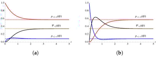
Figure 2. The probabilities $p_{j,-1}\left(t\right|0)$, $p_{j,-2}\left(t\right|0)$ and ${\mathcal{P}}_j\left(t\right|0)$ are plotted for $\phi \left(t\right)=1$ and for $\xi =1.0$, $\varrho =0.6$, $\nu =4.0$. In (a) $j=-2$ (failure state) and in (b) $j=-1$ (repair state).

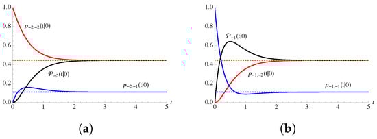
Figure 3. As in Figure 2, for $\phi \left(t\right)=1$ and for $\xi =1.0$, $\varrho =1.0$, $\nu =4.0$. In (a) $j=-2$ (failure state) and in (b) $j=-1$ (repair state).

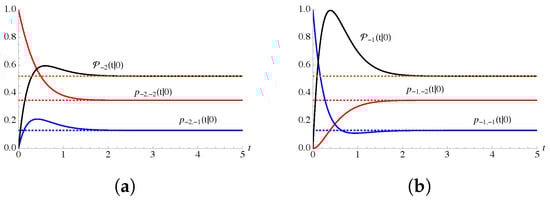
Figure 4. As in Figure 2, for $\phi \left(t\right)=1$ and for $\xi =1.0$, $\varrho =1.5$, $\nu =4.0$. In (a) $j=-2$ (failure state) and in (b) $j=-1$ (repair state).

4. Time of First Failure

We denote by

$${\mathcal{T}}_{j,-2}\left(t_0\right)=inf\{t>t_0:N\left(t\right)=-2\},j\in \{-1,0,1,\dots ,\ell \}$$

(20)

the random variable that describes the time of first failure of the system, i.e. the time in which the chain enters in the state F for the first time, starting from the state $j\in \{-1,0,1,\dots ,\ell \}$ at time $t_0$. Let

$$g_{j,-2}\left(t\right|t_0)=\frac{d}{dt}P({\mathcal{T}}_{j,-2}\left(t_0\right)\le t|N\left(t_0\right)=j),j\in \{-1,0,1,\dots ,\ell \}$$

(21)

be the density of the time of first failure.

Proposition 3.

Under the assumptions (11), for $j\in \{-1,0,1,\dots ,\ell \}$ one has

$$g_{j,-2}\left(t\right|t_0)=\left\{\begin{array}{cc}\xi \phi \left(t\right)\frac{\nu {\delta }_{j,-1}{e}^{-\nu \mathsf{\Phi }\left(t\right|t_0)}+\left[\xi (1-{\delta }_{j,-1})-\nu \right]e^{-\xi \mathsf{\Phi }\left(t\right|t_0)}}{\xi -\nu },\hfill & \nu \ne \xi ,\hfill \\ \\ \xi \phi \left(t\right)e^{-\xi \mathsf{\Phi }\left(t\right|t_0)}\left[1-{\delta }_{j,-1}+\xi \mathsf{\Phi }\left(t\right|t_0){\delta }_{j,-1}\right],\hfill & \nu =\xi .\hfill \end{array}\right.$$

(22)

Proof. 

We consider a time-inhomogeneous Markov process $\{\widehat{N}\left(t\right),t\ge t_0\}$ with state-space $\mathcal{S}$ obtained from $N\left(t\right)$ by setting an absorbing boundary into the state $-2$, that corresponds to the failure state F of the system and we denote by

$${\widehat{p}}_{j,n}\left(t\right|t_0)=P\{\widehat{N}\left(t\right)=n|\widehat{N}\left(t_0\right)=j\},j,n\in \mathcal{S}.$$

(23)

the probability that the system is in state n at time t and that no failure has yet occurred. Since,

$$P\{{\mathcal{T}}_{j,-2}\left(t_0\right)\le t\}+{\widehat{p}}_{j,-1}\left(t\right|t_0)+\sum _{n=0}^{\ell }{\widehat{p}}_{j,n}\left(t\right|t_0)=1,t\ge t_0,$$

one has $P\{{\mathcal{T}}_{j,-2}\left(t_0\right)\le t\}={\widehat{p}}_{j,-2}\left(t\right|t_0)$, so that for $t\ge t_0$ it results

$$g_{j,-2}\left(t\right|t_0)=\frac{d}{dt}{\widehat{p}}_{j,-2}\left(t\right|t_0),j\in \{-1,0,1,\dots ,\ell \}.$$

(24)

Hence, to determine the density of the time of first failure, it is necessary to consider the following differential equations

$$\begin{array}{ccc}& & \frac{d{\widehat{p}}_{j,-2}\left(t\right|t_0)}{dt}=\xi \phi \left(t\right)[1-{\widehat{p}}_{j,-1}\left(t\right|t_0)-{\widehat{p}}_{j,-2}\left(t\right|t_0)],\hfill \\ & & \frac{d{\widehat{p}}_{j,-1}\left(t\right|t_0)}{dt}=-\nu \phi \left(t\right){\widehat{p}}_{j,-1}\left(t\right|t_0),\hfill \\ & & \frac{d{\widehat{p}}_{j,0}\left(t\right|t_0)}{dt}={\gamma }_0\phi \left(t\right){\widehat{p}}_{j,-1}\left(t\right|t_0)-[{\lambda }_0\left(t\right)+\xi \phi \left(t\right)]{\widehat{p}}_{j,0}\left(t\right|t_0)+{\mu }_1\left(t\right){\widehat{p}}_{j,1}\left(t\right|t_0),\hfill \\ & & \frac{d{\widehat{p}}_{j,n}\left(t\right|t_0)}{dt}={\gamma }_n\phi \left(t\right){\widehat{p}}_{j,-1}\left(t\right|t_0)+{\lambda }_{n-1}\left(t\right){\widehat{p}}_{j,n-1}\left(t\right|t_0)\hfill \\ & & -[{\lambda }_n\left(t\right)+{\mu }_n\left(t\right)+\xi \phi \left(t\right)]{\widehat{p}}_{j,n}\left(t\right|t_0)+{\mu }_{n+1}\left(t\right){\widehat{p}}_{j,n+1}\left(t\right|t_0),n=1,2,\dots ,\ell -1,\hfill \\ & & \frac{d{\widehat{p}}_{j,\ell }\left(t\right|t_0)}{dt}={\gamma }_{\ell }\phi \left(t\right){\widehat{p}}_{j,-1}\left(t\right|t_0)+{\lambda }_{\ell -1}\left(t\right){\widehat{p}}_{j,\ell -1}\left(t\right|t_0)-[{\mu }_{\ell }\left(t\right)+\xi \phi \left(t\right)]{\widehat{p}}_{j,\ell }\left(t\right|t_0),\hfill \end{array}$$

(25)

to solve with the initial conditions

$$\underset{t\downarrow t_0}{lim}{\widehat{p}}_{j,n}\left(t\right|t_0)={\delta }_{j,n},j,n\in \mathcal{S},j\ne -2,\underset{t\downarrow t_0}{lim}{\widehat{p}}_{-2,n}\left(t\right|t_0)=0,n\in \mathcal{S}.$$

(26)

Proceeding as in Proposition 2, one has:

$${\widehat{p}}_{j,-2}\left(t\right|t_0)=\left\{\begin{array}{cc}\frac{\xi \left[1-e^{-\nu \mathsf{\Phi }\left(t\right|t_0)}\right]-\nu \left[1-e^{-\xi \mathsf{\Phi }\left(t\right|t_0)}\right]+\xi (1-{\delta }_{j,-1})\left[e^{-\nu \mathsf{\Phi }\left(t\right|t_0)}-e^{-\xi \mathsf{\Phi }\left(t\right|t_0)}\right]}{\xi -\nu },\hfill & \nu \ne \xi ,\hfill \\ \\ 1-e^{-\xi \mathsf{\Phi }\left(t\right|t_0)}\left[1+\xi \mathsf{\Phi }\left(t\right|t_0){\delta }_{j,-1}\right],\hfill & \nu =\xi ,\hfill \end{array}\right.$$

(27)

so that, by virtue of (24), Equation (22) holds. □

From (22) it follows that $P\{{\mathcal{T}}_{j,-2}\left(t_0\right)\le +\infty \}=1$, so that with certainty the system is destined to fail. By virtue of (24), for $j\in \{-1,0,1,\dots ,\ell \}$ the reliability of the system before the first repair is

$$\begin{array}{ccc}& & P\{{\mathcal{T}}_{j,-2}\left(t_0\right)>t\}={\int }_t^{+\infty }{g}_{j,-2}\left(\tau \right|t_0)d\tau ={\int }_t^{+\infty }\frac{d}{d\tau }{\widehat{p}}_{j,-2}\left(\tau \right|t_0)d\tau =1-{\widehat{p}}_{j,-2}\left(t\right|t_0)\hfill \\ & & =\left\{\begin{array}{cc}\frac{\xi {\delta }_{j,-1}{e}^{-\nu \mathsf{\Phi }\left(t\right|t_0)}+[\xi (1-{\delta }_{j,-1})-\nu ]e^{-\xi \mathsf{\Phi }\left(t\right|t_0)}}{\xi -\nu },\hfill & \nu \ne \xi ,\hfill \\ \\ \left[1+\xi \mathsf{\Phi }\left(t\right|t_0){\delta }_{j,-1}\right]e^{-\xi \mathsf{\Phi }\left(t\right|t_0)},\hfill & \nu =\xi .\hfill \end{array}\right.\hfill \end{array}$$

(28)

Hence, for $j\in \{-1,0,1,\dots ,\ell \}$ the mean time to first failure is

$$\begin{array}{ccc}& & E\left[{\mathcal{T}}_{j,-2}\left(t_0\right)\right]={\int }_{t_0}^{+\infty }(t-t_0)g_{j,-2}\left(t\right|t_0)dt={\int }_{t_0}^{+\infty }P\{{\mathcal{T}}_{j,-2}\left(t_0\right)>t\}dt\hfill \\ & & =\left\{\begin{array}{cc}\frac{\xi }{\xi -\nu }{\delta }_{j,-1}{\int }_{t_0}^{+\infty }{e}^{-\nu \mathsf{\Phi }\left(t\right|t_0)}dt+\frac{\xi (1-{\delta }_{j,-1})-\nu }{\xi -\nu }{\int }_{t_0}^{+\infty }{e}^{-\xi \mathsf{\Phi }\left(t\right|t_0)}dt,\hfill & \nu \ne \xi ,\hfill \\ \\ {\int }_{t_0}^{+\infty }{e}^{-\nu \mathsf{\Phi }\left(t\right|t_0)}\left[1+\xi {\delta }_{j,-1}\mathsf{\Phi }\left(t\right|t_0)\right]dt,\hfill & \nu =\xi .\hfill \end{array}\right.\hfill \end{array}$$

(29)

In particular, by setting $\phi \left(t\right)=1$, Equation (29) leads to

$$E\left[{\mathcal{T}}_{j,-2}\right]=\frac{1}{\nu }{\delta }_{j,-1}+\frac{1}{\xi },j\in \{-1,0,1,\dots ,\ell \}.$$

In Figure 5 the density of the time of first failure is plotted for $\phi \left(t\right)=1$, $\xi =1.0$, $\varrho =0.6$, $\nu =4.0$. If $j=-1$ one has $E\left[{\mathcal{T}}_{-1,-2}\right]=1.25$, whereas $E\left[{\mathcal{T}}_{j,-2}\right]=1$ if j is an operating state.

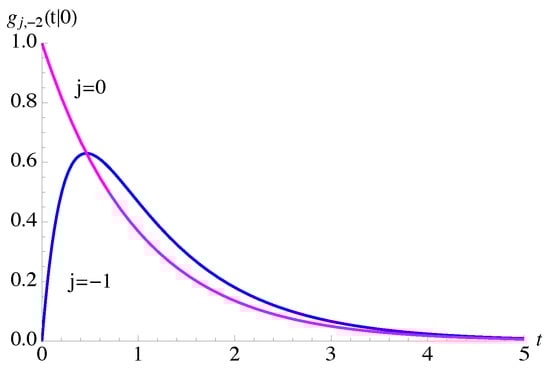
Figure 5. The density of the time of first failure is plotted for $\phi \left(t\right)=1$ and for $\xi =1.0$, $\varrho =0.6$, $\nu =4.0$.

5. Operating States and Their Probabilities

For the birth-death chain $\{N\left(t\right),t\ge t_0\}$, in addition to the assumptions (11), we suppose that the birth and death intensity functions are

$${\lambda }_n\left(t\right)=(\ell -n)\lambda \left(t\right),n=0,1,\dots ,\ell ;{\mu }_n\left(t\right)=n\mu \left(t\right),n=1,\dots ,\ell ,$$

(30)

with $\lambda \left(t\right)$ and $\mu \left(t\right)$ positive, bounded and continuous functions for $t\ge 0$. Note that the birth-death intensity functions (30) define a time-inhomogeneous Prendiville process $\{\tilde{N}\left(t\right),t\ge t_0\}$ with finite state-space $\{0,1,\dots ,\ell \}$. The process $\tilde{N}\left(t\right)$ identifies with the process $N\left(t\right)$ in the absence of failures, repairs and restores.

Under the assumptions (11) and (30), the transition probabilities of $N\left(t\right)$ satisfy the following system:

$$\begin{array}{ccc}& & \frac{d{p}_{j,0}\left(t\right|t_0)}{dt}={\gamma }_0\phi \left(t\right)p_{j,-1}\left(t\right|t_0)-[\ell \lambda \left(t\right)+\xi \phi \left(t\right)]p_{j,0}\left(t\right|t_0)+\mu \left(t\right)p_{j,1}\left(t\right|t_0),\hfill \\ & & \frac{d{p}_{j,n}\left(t\right|t_0)}{dt}={\gamma }_n\phi \left(t\right)p_{j,-1}\left(t\right|t_0)+\lambda \left(t\right)(\ell -n+1)p_{j,n-1}\left(t\right|t_0)\hfill \\ & & -[\lambda \left(t\right)(\ell -n)+\mu \left(t\right)n+\xi \phi \left(t\right)]p_{j,n}\left(t\right|t_0)+\mu \left(t\right)(n+1)p_{j,n+1}\left(t\right|t_0),\hfill \\ & & n=1,2,\dots ,\ell -1,\hfill \\ & & \frac{d{p}_{j,\ell }\left(t\right|t_0)}{dt}={\gamma }_{\ell }\phi \left(t\right)p_{j,-1}\left(t\right|t_0)+\lambda \left(t\right)p_{j,\ell -1}\left(t\right|t_0)-[\ell \mu \left(t\right)+\xi \phi \left(t\right)]p_{j,\ell }\left(t\right|t_0),\hfill \end{array}$$

(31)

to solve with the initial conditions

$$\underset{t\downarrow t_0}{lim}{p}_{j,n}\left(t\right|t_0)={\delta }_{j,n},j\in \mathcal{S},n\in \{0,1,\dots ,\ell \}.$$

(32)

Let

$$G_j(z,t)=\sum _{n=0}^{\ell }{z}^n{p}_{i,n}\left(t\right|t_0),j\in \mathcal{S}$$

(33)

be the probability generating function (PGF) of the operating states of $N\left(t\right)$. From (31) one has:

$$\begin{array}{ccc}& & \frac{\partial }{\partial t}{G}_j(z,t)+(z-1)[\lambda \left(t\right)z+\mu \left(t\right)]\frac{\partial }{\partial z}{G}_j(z,t)\hfill \\ & & =[\ell (z-1)\lambda \left(t\right)-\xi \phi \left(t\right)]G_j(z,t)+\phi \left(t\right)p_{j,-1}\left(t\right|t_0)\sum _{i=0}^{\ell }{\gamma }_i{z}^i,j\in \mathcal{S},\hfill \end{array}$$

(34)

to solve with the conditions

$$\begin{array}{ccc}& & G_j(z,t_0)=\sum _{n=0}^{\ell }{\delta }_{j,n}{z}^n=\left\{\begin{array}{cc}0,\hfill & j=-1,-2\hfill \\ z^j,\hfill & j\in \{0,1,\dots ,\ell \},\hfill \end{array}\right.\hfill \\ & & \hfill \\ & & G_j(z,t_0)=\mathcal{P}\left(t\right|t_0)=1-p_{j,-2}\left(t\right|t_0)-p_{j,-1}\left(t\right|t_0).\hfill \end{array}$$

(35)

Proposition 4.

Under the assumption (11) and (30), the PGF of the operating states of $N\left(t\right)$ is

$$\begin{array}{ccc}& & G_j(z,t)=e^{-\xi \mathsf{\Phi }\left(t\right|t_0)}\sum _{i=0}^{\ell }{\delta }_{j,i}{[1+(z-1)b_1\left(t\right|t_0)]}^i{[1+(z-1)b_2\left(t\right|t_0)]}^{\ell -i}\hfill \\ & & +{\int }_{t_0}^{t}du\phi \left(u\right)p_{j,-1}\left(u\right|t_0)e^{-\xi \mathsf{\Phi }\left(t\right|u)}{\left[\frac{1+(z-1)b_2\left(t\right|t_0)}{1+(z-1)b_2\left(u\right|t_0)}\right]}^{\ell }\hfill \\ & & \times \sum _{i=0}^{\ell }{\gamma }_i{\left[\frac{1+(z-1)b_1\left(t\right|u)}{1+(z-1)b_2\left(t\right|u)}\right]}^i,j\in \mathcal{S},\hfill \end{array}$$

(36)

where $\mathsf{\Phi }\left(t\right|t_0)$ is given in (12) and where

$$b_1\left(t\right|t_0)=e^{-[\mathsf{\Lambda }\left(t\right|t_0)+M\left(t\right|t_0)]}\left[1+B\left(t\right|t_0)\right],b_2\left(t\right|t_0)=e^{-[\mathsf{\Lambda }\left(t\right|t_0)+M\left(t\right|t_0)]}B\left(t\right|t_0),$$

(37)

with

$$\mathsf{\Lambda }\left(t\right|t_0)={\int }_{t_0}^t\lambda \left(\tau \right)d\tau ,M\left(t\right|t_0)={\int }_{t_0}^t\mu \left(\tau \right)d\tau ,B\left(t\right|t_0)={\int }_{t_0}^t\lambda \left(\tau \right)e^{\mathsf{\Lambda }\left(\tau \right|t_0)+M\left(\tau \right|t_0)}d\tau .$$

(38)

Proof. 

The proof is given in Appendix A. □

We remark that $0\le b_1\left(t\right|t_0)\le 1$ and $0\le b_2\left(t\right|t_0)\le 1$ for all $t\ge t_0$. Furthermore, we note that the function

$${\tilde{G}}_i(z,t)={\left[1+(z-1)b_1\left(t\right|t_0)\right]}^i{\left[1+(z-1)b_2\left(t\right|t_0)\right]}^{\ell -i},i\in \{0,1,\dots ,\ell \},$$

(39)

which appears to the right-hand sides of (36), is the PGF of the time-inhomogeneous Prendiville process $\tilde{N}\left(t\right)$, characterized by the birth-death intensity functions ${\lambda }_n\left(t\right)$ and ${\mu }_n\left(t\right)$, given in (30). The transition probabilities of $\tilde{N}\left(t\right)$ are (cf. Zheng [43], Giorno and Nobile [49]):

$$\begin{array}{cc}\hfill & {\tilde{p}}_{0,n}\left(t\right|t_0)=\left(\genfrac{}{}{0pt}{}{\ell }{n}\right){\left[b_2\left(t\right|t_0)\right]}^n{[1-b_2\left(t\right|t_0)]}^{\ell -n},\hfill \\ \hfill & {\tilde{p}}_{i,n}\left(t\right|t_0)={\left[b_1\left(t\right|t_0)\right]}^n{[1-b_2\left(t\right|t_0)]}^{\ell -i}{[1-b_1\left(t\right|t_0)]}^{i-n}\hfill \\ \hfill & \times \sum _{r=max(0,n-i)}^{min(\ell -i,n)}\left(\genfrac{}{}{0pt}{}{\ell -i}{r}\right)\left(\genfrac{}{}{0pt}{}{i}{n-r}\right){\left\{\frac{b_2\left(t\right|t_0)[1-b_1\left(t\right|t_0)]}{b_1\left(t\right|t_0)[1-b_2\left(t\right|t_0)]}\right\}}^r,i=1,2,\dots ,\ell -1,\hfill \\ \hfill & {\tilde{p}}_{\ell ,n}\left(t\right|t_0)=\left(\genfrac{}{}{0pt}{}{\ell }{n}\right){\left[b_1\left(t\right|t_0)\right]}^n{[1-b_1\left(t\right|t_0)]}^{\ell -n},\hfill \end{array}$$

(40)

and the conditional mean and the conditional variance are:

$$\begin{array}{cc}\hfill & \mathrm{E}\left[\tilde{N}\left(t\right)\right|\tilde{N}\left(t_0\right)=i]=i{b}_1\left(t\right|t_0)+(\ell -i)b_2\left(t\right|t_0),\hfill \\ \hfill & \mathrm{Var}\left[\tilde{N}\left(t\right)\right|\tilde{N}\left(t_0\right)=i]=i{b}_1\left(t\right|t_0)[1-b_1\left(t\right|t_0)]+(\ell -i)b_2\left(t\right|t_0)[1-b_2\left(t\right|t_0)].\hfill \end{array}$$

(41)

Under the assumptions (11) and (30), the probability that the system $N\left(t\right)$ is in the zero-state at time t can be determined from (33):

$$\begin{array}{ccc}& & p_{j,0}\left(t\right|t_0)=G_j(0,t)=e^{-\xi \mathsf{\Phi }\left(t\right|t_0)}\sum _{i=0}^{\ell }{\delta }_{j,i}{\tilde{p}}_{i,0}\left(t\right|t_0)\hfill \\ & & +\sum _{i=0}^{\ell }{\gamma }_i{\int }_{t_0}^{t}du\phi \left(u\right)p_{j,-1}\left(u\right|t_0)e^{-\xi \mathsf{\Phi }\left(t\right|u)}{\left[\frac{1-b_2\left(t\right|t_0)}{1-b_2\left(u\right|t_0)}\right]}^{\ell }{\left[\frac{1-b_1\left(t\right|u)}{1-b_2\left(t\right|u)}\right]}^i,j\in \mathcal{S},\hfill \end{array}$$

(42)

where

$${\tilde{p}}_{i,0}\left(t\right|t_0)={[1-b_1\left(t\right|t_0)]}^i{[1-b_2\left(t\right|t_0)]}^{\ell -i}$$

is obtained from (40). Similarly, the probability that the system $N\left(t\right)$ is in the state $n=1$ at time t follows from (36):

$$\begin{array}{ccc}& & p_{j,1}\left(t\right|t_0)=\frac{d{G}_j(z,t)}{dz}{|}_{z=0}=e^{-\xi \mathsf{\Phi }\left(t\right|t_0)}\sum _{i=0}^{\ell }{\delta }_{j,i}{\tilde{p}}_{i,1}\left(t\right|t_0)\hfill \\ & & +{\int }_{t_0}^{t}du\phi \left(u\right)p_{j,-1}\left(u\right|t_0)e^{-\xi \mathsf{\Phi }\left(t\right|u)}{\left[\frac{1-b_1\left(t\right|t_0)}{1-b_2\left(u\right|t_0)}\right]}^{\ell -1}\{\frac{\ell \left[b_2\left(t\right|t_0)-b_2\left(u\right|t_0)\right]}{{[1-b_2\left(u\right|t_0)]}^2}\hfill \\ & & \times \sum _{i=0}^{\ell }{\gamma }_i{\left[\frac{1-b_1\left(t\right|u)}{1-b_2\left(t\right|u)}\right]}^i+e^{-\left[\mathsf{\Lambda }\right(t\left|u\right)+M\left(t\right|u\left)\right]}\frac{1-b_1\left(t\right|t_0)}{1-b_2\left(u\right|t_0)}\sum _{i=0}^{\ell }i{\gamma }_i\frac{{[1-b_1\left(t\right|u)]}^{i-1}}{{[1-b_2\left(t\right|u)]}^{i+1}}\},\hfill \end{array}$$

(43)

where, by virtue of (40), one has:

$$\begin{array}{ccc}& & {\tilde{p}}_{i,1}\left(t\right|t_0)={[1-b_1\left(t\right|t_0)]}^{i-1}{[1-b_2\left(t\right|t_0)]}^{\ell -i-1}\hfill \\ & & \times \left\{i{b}_1\left(t\right|t_0)[1-b_2\left(t\right|t_0)]+(\ell -i)b_2\left(t\right|t_0)[1-b_1\left(t\right|t_0)]\right\}.\hfill \end{array}$$

For $r\in \mathbb{N}$, let us introduce the r-th conditional moment of $N\left(t\right)$:

$$\mathrm{E}\left[N^r\left(t\right)\right|N\left(t\right)\ge 0,N\left(t_0\right)=j]=\frac{1}{{\mathcal{P}}_j\left(t\right|t_0)}\sum _{n=0}^{\ell }{n}^r{p}_{j,n}\left(t\right|t_0),j\in \mathcal{S}.$$

(44)

From (36), we have

$$\begin{array}{ccc}& & \mathrm{E}\left[N\left(t\right)\right|N\left(t\right)\ge 0,N\left(t_0\right)=j]=\frac{1}{{\mathcal{P}}_j\left(t\right|t_0)}\frac{d{G}_j(z,t)}{dz}{|}_{z=1}\hfill \\ & & =\frac{1}{{\mathcal{P}}_j\left(t\right|t_0)}[e^{-\xi \mathsf{\Phi }\left(t\right|t_0)}\sum _{i=0}^{\ell }{\delta }_{j,i}\mathrm{E}\left[\tilde{N}\left(t\right)\right|\tilde{N}\left(t_0\right)=i]+{\int }_{t_0}^{t}du\phi \left(u\right)p_{j,-1}\left(u\right|t_0)e^{-\xi \mathsf{\Phi }\left(t\right|u)}\hfill \\ & & \times \left\{\ell \nu [b_2\left(t\right|t_0)-b_2\left(u\right|t_0)]+e^{-\left[\mathsf{\Lambda }\right(t\left|u\right)+M\left(t\right|u\left)\right]}\sum _{i=0}^{\ell }i{\gamma }_i\right\}],j\in \mathcal{S},\hfill \end{array}$$

(45)

where $\mathrm{E}\left[\tilde{N}\left(t\right)\right|\tilde{N}\left(t_0\right)=i]$ is given in (41).

6. Asymptotic Distribution of Operating States

To study the asymptotic behavior of the probabilities for the operating states, we assume that the intensity functions of $N\left(t\right)$ are proportional. Specifically, in addition to the conditions (11), we suppose that

$${\lambda }_n\left(t\right)=(\ell -n)\lambda \phi \left(t\right),n=0,1,\dots ,\ell ;{\mu }_n\left(t\right)=n\mu \phi \left(t\right),n=1,\dots ,\ell ,$$

(46)

with $\phi \left(t\right)$ positive, bounded and continuous function for $t\ge 0$.

Let

$$G\left(z\right)=\sum _{n=0}^{\ell }{z}^n{q}_n$$

(47)

be the asymptotic PGF of the operating states of $N\left(t\right)$. From (34) one has

$$(z-1)[\lambda z+\mu ]\frac{dG\left(z\right)}{dz}=[\ell (z-1)\lambda -\xi ]G\left(z\right)+q_{-1}\sum _{i=0}^{\ell }{\gamma }_i{z}^i,j\in \mathcal{S},$$

(48)

to solve with the condition

$$G\left(1\right)=Q=1-q_{-2}-q_{-1}.$$

(49)

Proposition 5.

Under the assumptions (11) and (46), the asymptotic PGF of the operating states is:

$$\begin{array}{ccc}& & G\left(z\right)={(\lambda z+\mu )}^{\xi /(\lambda +\mu )+\ell }{(1-z)}^{-\xi /(\lambda +\mu )}{q}_{-1}\hfill \\ & & \times \sum _{i=0}^{\ell }{\gamma }_i{\int }_z^1{x}^i{(\lambda x+\mu )}^{-\xi /(\lambda +\mu )-\ell -1}{(1-x)}^{\xi /(\lambda +\mu )-1}dx.\hfill \end{array}$$

(50)

Proof. 

The general solution of the differential Equation (48) is:

$$\begin{array}{ccc}& & G\left(z\right)={(\lambda z+\mu )}^{\xi /(\lambda +\mu )+\ell }{(1-z)}^{-\xi /(\lambda +\mu )}\hfill \\ & & \times \left[-q_{-1}\sum _{i=0}^{\ell }{\gamma }_i{\int }_{}^z{x}^i{(\lambda x+\mu )}^{-\xi /(\lambda +\mu )-\ell -1}{(1-x)}^{\xi /(\lambda +\mu )-1}dx+c\right],\hfill \end{array}$$

(51)

where c is an arbitrary constant. Making use of the condition (49), we note that the term in square brackets at the right-hand side of (51) must vanish when $z\to 1$, allowing to determine the constant c. Hence, from (51) we obtain (50). □

The knowledge of the asymptotic PGF (50) allows to calculate the asymptotic probabilities of the operating states, as

$$q_0=G\left(0\right),q_n=\frac{1}{n!}\frac{d^{n}G\left(z\right)}{d{z}^n}{|}_{z=0},n=1,2,\dots ,\ell ,$$

(52)

and the r-th asymptotic conditional moment of $N\left(t\right)$:

$$\mathrm{E}\left[N^r\right|N\ge 0]=\frac{1}{\mathcal{Q}}\sum _{n=0}^{\ell }{n}^r{q}_n,r\in \mathbb{N}.$$

(53)

Proposition 6.

Under the assumptions (11) and (46), one has:

$$\begin{array}{ccc}& & q_0=\frac{1}{\lambda +\mu }{\left(\frac{\mu }{\lambda +\mu }\right)}^{\xi /(\lambda +\mu )+\ell }{q}_{-1}\sum _{i=0}^{\ell }{\gamma }_{i}B\left(i+1,\frac{\xi }{\lambda +\mu }\right)\hfill \\ & & \times F\left(\frac{\xi }{\lambda +\mu },\frac{\xi }{\lambda +\mu }+\ell +1;\frac{\xi }{\lambda +\mu }+i+1;\frac{\lambda }{\lambda +\mu }\right),\hfill \\ & & q_1=\frac{1}{\mu }(\lambda \ell +\xi )q_0-\frac{{\gamma }_0}{\mu }{q}_{-1},\hfill \\ & & q_2=\frac{1}{2{\mu }^2}\{(\lambda \ell +\xi )[\lambda (\ell -1)+\xi ]+\xi \mu \}{q}_0+\left\{\frac{{\gamma }_0}{2{\mu }^2}\left[\lambda (\ell -1)+\xi +\mu \right]-\frac{{\gamma }_1}{2\mu }\right\}{q}_{-1},\hfill \end{array}$$

(54)

where

$$B(x,y)=\frac{\mathsf{\Gamma }\left(x\right)\mathsf{\Gamma }\left(y\right)}{\mathsf{\Gamma }(x+y)}$$

(55)

denotes the beta function and

$$F(a,b;c;x)=\sum _{n=0}^{+\infty }\frac{{\left(a\right)}_n{\left(b\right)}_n}{{\left(c\right)}_n}\frac{x^n}{n!}$$

(56)

is the Gauss hypergeometric function.

Proof. 

Since $q_0=G\left(0\right)$, by setting $z=0$ in (50) one obtains:

$$q_0={\mu }^{\ell +\xi /(\lambda +\mu )}{q}_{-1}\sum _{i=0}^{\ell }{\gamma }_i{\int }_0^1{x}^i{(\lambda x+\mu )}^{-\xi /(\lambda +\mu )-\ell -1}{(1-x)}^{\xi /(\lambda +\mu )-1}dx.$$

(57)

Recalling that (see, Gradshteyn and Ryzhik [50], p. 1005 and p. 1008, n. 9.131)

$$\begin{array}{ccc}& & F(a,b;c;z)=\frac{1}{B(b,c-b)}{\int }_0^1{x}^{b-1}{(1-x)}^{c-b-1}{(1-xz)}^{-a}dx,Rec>Reb>0,\hfill \\ & & F(a,b;c;z)={(1-z)}^{-a}F\left(a,c-b;c;\frac{z}{z-1}\right),\hfill \end{array}$$

by setting $a=\ell +1+\xi /(\lambda +\mu )$, $b=i+1$, $c=i+1+\xi /(\lambda +\mu )$ and $z=-\lambda /\mu$, for $i=0,1,\dots ,\ell$ one has

$$\begin{array}{ccc}& & {\int }_0^1{x}^i{(\lambda x+\mu )}^{-\xi /(\lambda +\mu )-\ell -1}{(1-x)}^{\xi /(\lambda +\mu )-1}dx={\mu }^{-\xi /(\lambda +\mu )-\ell -1}\hfill \\ & & \times B\left(i+1,\frac{\xi }{\lambda +\mu }\right)F\left(\frac{\xi }{\lambda +\mu }+\ell +1,i+1;\frac{\xi }{\lambda +\mu }+i+1:-\frac{\lambda }{\mu }\right)\hfill \\ & & ={(\lambda +\mu )}^{-\xi /(\lambda +\mu )-\ell -1}B\left(i+1,\frac{\xi }{\lambda +\mu }\right)F\left(\frac{\xi }{\lambda +\mu },\frac{\xi }{\lambda +\mu }+\ell +1;\frac{\xi }{\lambda +\mu }+i+1;\frac{\lambda }{\lambda +\mu }\right),\hfill \end{array}$$

where the symmetry property $F(a,b;c;z)=F(b,a;c;z)$ has been used in the last equality. Hence, the first equation in (54) follows from (57). Moreover, from (50) we have:

$$\frac{dG\left(z\right)}{dz}=\left[\left(\ell +\frac{\xi }{\lambda +\mu }\right)\frac{\lambda }{\lambda z+\mu }+\frac{\xi }{\lambda +\mu }\frac{1}{1-z}\right]G\left(z\right)-\frac{q_{-1}}{(\lambda z+\mu )(1-z)}\sum _{i=0}^{\ell }{\gamma }_i{z}^i,$$

(58)

so that the second equation in (54) follows from (52) for $n=1$. Finally, from (58) one has:

$$\begin{array}{ccc}& & \frac{d^{2}G\left(z\right)}{d{z}^2}=\left[-\left(\ell +\frac{\xi }{\lambda +\mu }\right){\left(\frac{\lambda }{\lambda z+\mu }\right)}^2+\frac{\xi }{\lambda +\mu }{\left(\frac{1}{1-z}\right)}^2\right]G\left(z\right)\hfill \\ & & +\left[\left(\ell +\frac{\xi }{\lambda +\mu }\right)\frac{\lambda }{\lambda z+\mu }+\frac{\xi }{\lambda +\mu }\frac{1}{1-z}\right]\frac{dG\left(z\right)}{dz}\hfill \\ & & +\frac{q_{-1}}{(\lambda z+\mu )(1-z)}\left[\left(\frac{\lambda }{\lambda z+\mu }-\frac{1}{1-z}\right)\sum _{i=0}^{\ell }{\gamma }_i{z}^i-\sum _{i=0}^{\ell }i{\gamma }_i{z}^{i-1}\right].\hfill \end{array}$$

(59)

Hence, by virtue of (52) for $n=2$, from (59) the last equation in (54) follows. □

Proposition 7.

Under the assumptions (11) and (46), one obtain:

$$\mathrm{E}\left[N\right|N\ge 0]=\frac{1}{\lambda +\mu +\xi }\left\{\lambda \ell +\frac{\xi }{\nu }\sum _{i=0}^{\ell }i{\gamma }_i\right\},$$

(60)

with $\nu ={\gamma }_0+{\gamma }_1+\dots +{\gamma }_{\ell }$.

Proof. 

By virtue of (53), from (58) one has

$$\begin{array}{ccc}& & \mathrm{E}\left[N\right|N\ge 0]=\frac{1}{Q}\frac{dG\left(z\right)}{dz}{|}_{z=1}\hfill \\ & & =\frac{1}{Q}\underset{z\to 1}{lim}\frac{\left[\left(\ell +\frac{\xi }{\lambda +\mu }\right)\frac{\lambda (1-z)}{\lambda z+\mu }+\frac{\xi }{\lambda +\mu }\right]G\left(z\right)-\frac{q_{-1}}{\lambda z+\mu }{\sum }_{i=0}^{\ell }{\gamma }_i{z}^i}{1-z}\hfill \\ & & =\left(\ell +\frac{\xi }{\lambda +\mu }\right)\frac{\lambda }{\lambda +\mu }-\frac{\xi }{\lambda +\mu }\mathrm{E}\left[N\right|N\ge 0]-\frac{q_{-1}}{Q}\frac{\lambda \nu }{{(\lambda +\mu )}^2}+\frac{q_{-1}}{Q(\lambda +\mu )}\sum _{i=0}^{\ell }i{\gamma }_i\hfill \end{array}$$

from which (60) follows. □

Example 1.

We assume that $\ell =0$. Under the assumptions (11), the time-inhomogeneous Markov chain $N\left(t\right)$ is shown in Figure 6.

Figure 6. The state diagram of the Markov process $N\left(t\right)$ with $\ell =0$.

In this case, there is only one operating state in zero, the intensity functions of failure $\xi \left(t\right)=\xi \phi \left(t\right)$, of repair $\varrho \left(t\right)=\varrho \phi \left(t\right)$ and of restore ${\gamma }_0\left(t\right)={\gamma }_0\phi \left(t\right)$ are proportional and $p_{j,0}\left(t\right|t_0)+p_{j,-2}\left(t\right|t_0)+p_{j,-1}\left(t\right|t_0)=1$. From (42), one has:

$$p_{j,0}\left(t\right|t_0)=e^{-\xi \mathsf{\Phi }\left(t\right|t_0)}{\delta }_{j,0}+{\gamma }_0{\int }_{t_0}^t\phi \left(u\right)p_{j,-1}\left(u\right|t_0)e^{-\xi \mathsf{\Phi }\left(t\right|u)}du,j=-2,-1,0.$$

(61)

Of course, the conditional mean (45) is equal to zero for all $t\ge t_0$.

From Proposition 6, one obtains:

$$q_0=\frac{1}{\xi }{\left(\frac{\mu }{\lambda +\mu }\right)}^{\xi /(\lambda +\mu )}{q}_{-1}F\left(\frac{\xi }{\lambda +\mu },\frac{\xi }{\lambda +\mu }+1;\frac{\xi }{\lambda +\mu }+1;\frac{\lambda }{\lambda +\mu }\right).$$

(62)

Since,

$$F(a,b;b;z)={(1-z)}^{-a},$$

(63)

from (62) one clearly has

$$q_0=\frac{q_{-1}}{\xi }{\gamma }_0=\frac{\varrho {\gamma }_0}{{\gamma }_0\varrho +{\gamma }_0\xi +\varrho \xi },$$

that identifies with the probability Q, being $\nu ={\gamma }_0$.

Example 2.

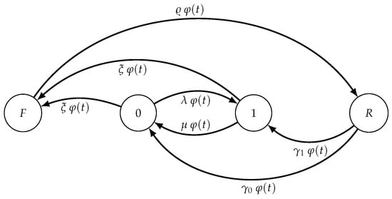
We assume that $\ell =1$. Under the assumption (11) and (46), the time-inhomogeneous Markov chain $N\left(t\right)$ is shown in Figure 7.

Figure 7. The state diagram of the Markov chain $N\left(t\right)$ with $\ell =1$.

In this case, there are two operating states 0 and 1, with intensity functions of failure $\xi \left(t\right)=\xi \phi \left(t\right)$, of repair $\varrho \left(t\right)=\varrho \phi \left(t\right)$ and of restores ${\gamma }_i\left(t\right)={\gamma }_i\phi \left(t\right)$ for $i=0,1$; the birth-death intensity functions are ${\lambda }_0\left(t\right)=\lambda \phi \left(t\right)$ and ${\mu }_1\left(t\right)=\mu \phi \left(t\right)$. By setting $\ell =1$ in the first equation in of (54) one has

$$\begin{array}{ccc}& & q_0=\frac{1}{\xi }{\left(\frac{\mu }{\lambda +\mu }\right)}^{\xi /(\lambda +\mu )+1}{q}_{-1}[{\gamma }_{0}F\left(\frac{\xi }{\lambda +\mu },\frac{\xi }{\lambda +\mu }+2;\frac{\xi }{\lambda +\mu }+1;\frac{\lambda }{\lambda +\mu }\right)\hfill \\ & & +{\gamma }_1\frac{\lambda +\mu }{\lambda +\mu +\xi }F\left(\frac{\xi }{\lambda +\mu },\frac{\xi }{\lambda +\mu }+2;\frac{\xi }{\lambda +\mu }+2;\frac{\lambda }{\lambda +\mu }\right)].\hfill \end{array}$$

(64)

Recalling the Gauss’ recursion function (see, Gradshteyn and Ryzhik [50], p. 1010, n. 9.137.17)

$$cF(a,b;c;z)-(c-b)F(a,b;c+1;z)-bF(a,b+1;c+1;z)=0$$

(65)

and the relation (63), one obtains:

$$F\left(\frac{\xi }{\lambda +\mu },\frac{\xi }{\lambda +\mu }+2;\frac{\xi }{\lambda +\mu }+1;\frac{\lambda }{\lambda +\mu }\right)=\frac{\lambda +\mu }{\lambda +\mu +\xi }\frac{\mu +\xi }{\mu }{\left(\frac{\mu }{\lambda +\beta }\right)}^{-\xi /(\lambda +\mu )}$$

(66)

Making use of (66) and of the relation (63) in Equation (64), for $\ell =1$ it follows

$$\begin{array}{ccc}& & q_0=\frac{\mu }{\xi }\frac{1}{\lambda +\mu +\xi }\left[\left(1+\frac{\xi }{\mu }\right){\gamma }_0+{\gamma }_1\right]q_{-1},\hfill \\ & & \hfill \\ & & q_1=\frac{\lambda +\xi }{\mu }{q}_0-\frac{{\gamma }_0}{\mu }{q}_{-1}.\hfill \end{array}$$

(67)

Of course, $q_0+q_1=Q=\varrho \nu /(\varrho \nu +\nu \xi +\varrho \xi )$, with $\nu ={\gamma }_0+{\gamma }_1$. From (53) we have

$$\mathrm{E}\left(N\right|N\ge 0)=\frac{q_1}{Q}=\frac{\lambda +\xi }{\mu }\frac{q_0}{Q}-\frac{{\gamma }_0}{\mu }\frac{\xi }{{\gamma }_0+{\gamma }_1}=\frac{1}{\lambda +\mu +\xi }\left(\lambda +\xi \frac{{\gamma }_1}{{\gamma }_0+{\gamma }_1}\right).$$

that identifies with (60) for $\ell =1$.

Example 3.

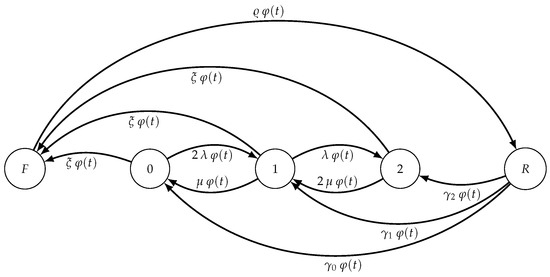
We assume that $\ell =2$. Under the assumption (11) and (46), the time-inhomogeneous Markov chain $N\left(t\right)$ is shown in Figure 8.

Figure 8. The state diagram of the Markov chain $N\left(t\right)$ with $\ell =2$.

In this case, there are three operating states 0, 1 and 2, with the intensity functions of failure $\xi \left(t\right)=\xi \phi \left(t\right)$, of repair $\varrho \left(t\right)=\varrho \phi \left(t\right)$ and of restores ${\gamma }_i\left(t\right)={\gamma }_i\phi \left(t\right)$ for $i=0,1,2$; the birth-death intensity functions are ${\lambda }_n\left(t\right)=(2-n)\lambda \phi \left(t\right)$ for $n=0,1$ and ${\mu }_n\left(t\right)=n\mu \phi \left(t\right)$ for $n=1,2$. By setting $\ell =2$ in the first equation in of (54) one obtains

$$\begin{array}{ccc}& & q_0=\frac{1}{\xi }{\left(\frac{\mu }{\lambda +\mu }\right)}^{\xi /(\lambda +\mu )+2}{q}_{-1}[{\gamma }_{0}F\left(\frac{\xi }{\lambda +\mu },\frac{\xi }{\lambda +\mu }+3;\frac{\xi }{\lambda +\mu }+1;\frac{\lambda }{\lambda +\mu }\right)\hfill \\ & & +{\gamma }_1\frac{\lambda +\mu }{\lambda +\mu +\xi }F(\frac{\xi }{\lambda +\mu },\frac{\xi }{\lambda +\mu }+3;\frac{\xi }{\lambda +\mu }+2;\frac{\lambda }{\lambda +\mu }\hfill \\ & & +2{\gamma }_2\frac{{(\lambda +\mu )}^2}{(\lambda +\mu +\xi )\left[2\right(\lambda +\mu )+\xi ]}F\left(\frac{\xi }{\lambda +\mu },\frac{\xi }{\lambda +\mu }+3;\frac{\xi }{\lambda +\mu }+3;\frac{\lambda }{\lambda +\mu }\right)].\hfill \end{array}$$

(68)

By virtue of (65), one has:

$$\begin{array}{ccc}& & F\left(\frac{\xi }{\lambda +\mu },\frac{\xi }{\lambda +\mu }+3;\frac{\xi }{\lambda +\mu }+1;\frac{\lambda }{\lambda +\mu }\right)=\frac{{(\lambda +\mu )}^2}{2(\lambda +\mu )+\xi }{\left(\frac{\mu }{\lambda +\beta }\right)}^{-\xi /(\lambda +\mu )}\hfill \\ & & \times \left[\frac{\xi }{{\mu }^2}+\frac{2}{\lambda +\mu +\xi }\left(1+\frac{\xi }{\mu }\right)\right],\hfill \\ & & \hfill \\ & & F\left(\frac{\xi }{\lambda +\mu },\frac{\xi }{\lambda +\mu }+3;\frac{\xi }{\lambda +\mu }+2;\frac{\lambda }{\lambda +\mu }\right)=\frac{\lambda +\mu }{2(\lambda +\mu )+\xi }{\left(\frac{\mu }{\lambda +\beta }\right)}^{-\xi /(\lambda +\mu )}\left(2+\frac{\xi }{\mu }\right),\hfill \end{array}$$

(69)

Making use of (69) and of the relation (63) in Equation (68), for $\ell =2$ it follows

$$\begin{array}{ccc}& & q_0=\frac{{\mu }^2}{\xi }\frac{1}{(\lambda +\mu +\xi )\left[2\right(\lambda +\mu )+\xi ]}{q}_{-1}\hfill \\ & & \times \left\{{\gamma }_0\right[\frac{\xi (\lambda +\mu +\xi )}{{\mu }^2}+2(1+\frac{\xi }{\mu })]+{\gamma }_1(2+\frac{\xi }{\mu })+2{\gamma }_2\},\hfill \\ & & q_1=\frac{2\lambda +\xi }{\mu }{q}_0-\frac{{\gamma }_0}{\mu }{q}_{-1},\hfill \\ & & q_2=\frac{(\xi +\lambda )(\xi +2\lambda )+\xi \mu }{2{\mu }^2}{q}_0-\left[{\gamma }_0\frac{\xi +\lambda +\mu }{2{\mu }^2}+\frac{{\gamma }_1}{2\mu }\right]q_{-1}.\hfill \end{array}$$

(70)

Clearly, $q_0+q_1+q_2=Q=\varrho \nu /(\varrho \nu +\nu \xi +\varrho \xi )$, with $\nu ={\gamma }_0+{\gamma }_1+{\gamma }_2$. Finally, from (53) one obtains

$$\begin{array}{ccc}& & \mathrm{E}\left(N\right|N\ge 0)=\frac{q_1+2q_2}{Q}=\left[\frac{2\lambda +\xi }{\mu }+\frac{(\xi +\lambda )(\xi +2\lambda )+\xi \mu }{{\mu }^2}\right]\frac{q_0}{Q}\hfill \\ & & -\left[{\gamma }_0\frac{\xi +\lambda +2\mu }{{\mu }^2}+\frac{{\gamma }_1}{\mu }\right]\frac{\xi }{{\gamma }_0+{\gamma }_1+{\gamma }_2}=\frac{1}{\lambda +\mu +\xi }\left\{2\lambda +\xi \frac{{\gamma }_1+2{\gamma }_2}{{\gamma }_0+{\gamma }_1+{\gamma }_2}\right\},\hfill \end{array}$$

that identifies with (60) for $\ell =2$.

7. Conclusions

In the present paper, we have considered a time-inhomogeneous CTMC with a finite space-state in which failures and repairs can occur at random times. In addition to the operating states, the space of the states includes two particular ones, denoted by F and R, representing the failure state and the repair one, respectively. The failures occur according to a non-stationary exponential distribution and they produce a transition from an operating state to F. Subsequently, a repair is required that involves a transition from F to R. Even the repair times are assumed to be random and occurring according to a non-stationary exponential distribution. After the reparation, the system restarts from one of the operating states.

Assuming that the failures, repairs and restores are characterized by proportional intensity functions, we determine the transition probabilities that, starting from an arbitrary state j at time $t_0$, the system reaches the state F, or the state R, or one of the operating states at time t. The obtained results show that that the probability that the system is in an operating state at time t does not depend on the intensity functions related to the birth-death process without failures and repairs. In other words, the transition probabilities related to the states F, R, as well as the transition probability that the system occupies an operating state, are independent of the dynamics existing between the operating states. We determine the density of the time of first failure and the related average. Moreover, we focus on the transition probabilities of operating states by determining the PGF and the conditioned mean. Finally, under the assumption of proportional intensity functions, we analyze the asymptotic behavior for the probabilities of the operating states by calculating the asymptotic PGF and the asymptotic conditional mean.

References

- Anderson, W.J. Continuous-Time Markov Chains: An Applications-Oriented Approach; Springer Series in Statistics; Springer: New York, NY, USA, 1991. [Google Scholar]
- Iosifescu, M.; Tautu, P. Stochastic Processes and Applications in Biology and Medicine II. Models; Springer: Berlin/Heidelberg, Germany, 1973. [Google Scholar]
- Medhi, J. Stochastic Models in Queueing Theory; Academic Press: Amsterdam, The Netherlands, 2003. [Google Scholar]
- Bailey, N.T.J. The Elements of Stochastic Processes with Applications to the Natural Sciences; John Wiley & Sons, Inc.: New York, NY, USA, 1964. [Google Scholar]
- van Kampen, N.G. Stochastic Processes in Physics and Chemistry; Elsevier Science: Amsterdam, The Netherlands, 1992. [Google Scholar]
- Taylor, H.M.; Karlin, S. An Introduction to Stochastic Modeling; Academic Press: Boston, MA, USA, 1994. [Google Scholar]
- Sericola, B. Markov Chains: Theory, Algorithms and Applications; John Wiley & Sons, Inc.: Hoboken, NJ, USA, 2013. [Google Scholar]
- Dharmaraja, S.; Di Crescenzo, A.; Giorno, V.; Nobile, A.G. A continuous-time Ehrenfest model with catastrophes and its jump-diffusion approximation. J. Stat. Phys. 2015, 161, 326–345. [Google Scholar] [CrossRef]
- Giorno, V.; Nobile, A.G. On a bilateral linear birth and death process in the presence of catastrophe. In Computer Aided Systems Theory-EUROCAST 2013, Part I; Moreno-Diaz, R., Pichler, F., Quesada-Arencibia, A., Eds.; LNCS 8111; Springer: Berlin/Heidelberg, Germany, 2013; pp. 28–35. [Google Scholar]
- Giorno, V.; Nobile, A.G.; Spina, S. On some time non-homogeneous queueing systems with catastrophes. Appl. Math. Comp. 2014, 245, 220–234. [Google Scholar] [CrossRef]
- Giorno, V.; Nobile, A.G.; Pirozzi, E. A state-dependent queueing system with asymptotic logarithmic distribution. J. Math. Anal. Appl. 2018, 458, 949–966. [Google Scholar] [CrossRef]
- Di Crescenzo, A.; Giorno, V.; Nobile, A.G. Constructing transient birth-death processes by means of suitable transformations. Appl. Math. Comp. 2016, 281, 152–171. [Google Scholar] [CrossRef]
- Economou, A.; Fakinos, D. A continuous-time Markov chain under the influence of a regulating point process and applications in stochastic models with catastrophes. Eur. J. Oper. Res. 2003, 149, 625–640. [Google Scholar] [CrossRef]
- Economou, A.; Fakinos, D. Alternative approaches for the transient analysis of Markov chains with catastrophes. J. Stat. Theory Pract. 2008, 2, 183–197. [Google Scholar] [CrossRef][Green Version]
- Chen, A.; Zhang, H.; Liu, K.; Rennolls, K. Birth-death processes with disasters and instantaneous resurrection. Adv. Appl. Probab. 2004, 36, 267–292. [Google Scholar] [CrossRef]
- Di Crescenzo, A.; Giorno, V.; Krishna Kumar, B.; Nobile, A.G. A double-ended queue with catastrophes and repairs, and a jump-diffusion approximation. Method. Comput. Appl. Probab. 2012, 14, 937–954. [Google Scholar] [CrossRef]
- Di Crescenzo, A.; Giorno, V.; Krishna Kumar, B.; Nobile, A.G. A time-non-homogeneous double-ended queue with failures and repairs and its continuous approximation. Mathematics 2018, 6, 81. [Google Scholar] [CrossRef]
- Ye, J.; Liu, L.; Jiang, T. Analysis of a Single-Sever Queue with Disasters and Repairs Under Bernoulli Vacation Schedule. J. Syst. Sci. Inf. 2016, 4, 547–559. [Google Scholar] [CrossRef]
- Mytalas, G.C.; Zazanis, M.A. An MX/G/1 queueing system with disasters and repairs under a multiple adapted vacation policy. Nav. Res. Logist. 2015, 62, 171–189. [Google Scholar] [CrossRef]
- Krishna Kumar, B.K.; Krihnamoorthy, A.; Madheswari, S.P.; Basha, S.S. Transient analysis of a single server queue with catastrophes, failures, and repairs. Queueing Syst. 2007, 56, 133–141. [Google Scholar] [CrossRef]
- Altiok, T. On the phase-type approximations of general distributions. IIE Trans. 1985, 17, 110–116. [Google Scholar] [CrossRef]
- Altiok, T. Queueing modeling of a single processor with failures. Perform. Eval. 1989, 9, 93–102. [Google Scholar] [CrossRef]
- Altiok, T. Performance Analysis of Manufacturing Systems; Springer Series in Operations Research; Springer: New York, NY, USA, 1997. [Google Scholar]
- Dallery, Y. On modeling failure and repair times in stochastic models of manufacturing systems using generalized exponential distributions. Queueing Syst. 1994, 15, 199–209. [Google Scholar] [CrossRef]
- Kendall, D.G. On the generalized “birth-and-death”process. Ann. Math. Stat. 1948, 19, 1–15. [Google Scholar] [CrossRef]
- McNeil, D.R.; Schach, S. Central limit analogues for Markov population processes. J. R. Stat. Soc. Ser. B (Methodol.) 1973, 35, 1–23. [Google Scholar] [CrossRef]
- Di Crescenzo, A.; Nobile, A.G. Diffusion approximation to a queueing system with time dependent arrival and service rates. Queueing Syst. 1995, 19, 41–62. [Google Scholar] [CrossRef]
- Di Crescenzo, A.; Giorno, V.; Krishna Kumar, B.; Nobile, A.G. M/M/1 queue in two alternating environments and its heavy traffic approximation. J. Math. Anal. Appl. 2018, 458, 973–1001. [Google Scholar] [CrossRef]
- Giorno, V.; Nobile, A.G.; Ricciardi, L.M. On some time-nonhomogeneous diffusion approximations to queueing systems. Adv. Appl. Prob. 1987, 19, 974–994. [Google Scholar] [CrossRef]
- Giorno, V.; Nobile, A.G. On a class of birth-death processes with time-varying intensity functions. Appl. Math. Comput. 2020, 379, 125255. [Google Scholar] [CrossRef]
- Ammar, S.I.; Zeifman, A.; Satin, Y.; Kiseleva, K.; Koroley, V. On limiting characteristics for a non-stationary two–processor heterogeneous system with catastrophes, server failures and repairs. J. Ind. Manag. Optim. 2021, 17, 1057–1068. [Google Scholar] [CrossRef]
- Zeifman, A.I.; Isaacson, D.L. On strong ergodicity for nonhomogeneous continuous-time Markov chains. Stoch. Process. Appl. 1994, 50, 263–273. [Google Scholar] [CrossRef]
- Zeifman, A.; Satin, Y.; Korolev, V.; Shorgin, S. On truncations for weakly ergodic inhomogeneous birth and death processes. Int. J. Appl. Math. Comput. Sci. 2014, 24, 503–518. [Google Scholar] [CrossRef]
- Satin, Y.A.; Zeifman, A.I.; Shilova, G.N. On approaches to constructing limiting regimes for some queuing models. Inform. Primen. 2020, 14, 3–9. [Google Scholar]
- Jouini, O.; Dallery, Y. Moments of first passage times in general birth-death processes. Math. Meth. Oper. Res. 2008, 68, 49–76. [Google Scholar] [CrossRef]
- Giorno, V.; Nobile, A.G. First-passage times and related moments for continuous-time birth-death chains. Ric. Mat. 2019, 68, 629–659. [Google Scholar] [CrossRef]
- Prendiville, B.J. Discussion: Symposium on stochastic processes. J. Roy. Statist. Soc. B 1949, 11, 273. [Google Scholar]
- Takashima, M. Note on evolutionary processes. Bull. Math. Stat. 1956, 7, 18–24. [Google Scholar] [CrossRef]
- Giorno, V.; Negri, C.; Nobile, A.G. A solvable model for a finite capacity queueing system. J. Appl. Prob. 1985, 22, 903–911. [Google Scholar] [CrossRef]
- Ricciardi, L.M. Stochastic Population Theory: Birth and Death Processes. In Mathematical Ecology. Biomathematics; Hallam, T.G., Levin, S.A., Eds.; Springer: Berlin/Heidelberg, Germany, 1986; Volume 17, pp. 155–190. [Google Scholar]
- Karlin, S.; McGregor, J. Ehrenfest Urn Model. J. Appl. Prob. 1965, 2, 352–376. [Google Scholar] [CrossRef]
- Flegg, M.B.; Pollett, P.K.; Gramotnev, D.K. Ehrenfest model for condensation and evaporation processes in degrading aggregates with multiple bonds. Phys. Rev. E 2008, 78, 031117. [Google Scholar] [CrossRef]
- Zheng, Q. Note on the non-homogeneous Prendiville process. Math. Biosci. 1998, 148, 1–5. [Google Scholar] [CrossRef]
- Giorno, V.; Nobile, A.G.; Saura, A. Prendiville Stochastic Growth Model in the Presence of Catastrophes. In Cybernetics and Systems 2004, Proceedings of the 17th European Meeting on Cybernetics and Systems Research, Vienna, Austria, 13–16 April 2004; Trappl, R., Ed.; Austrian Society for Cybernetic Studies: Vienna, Austria, 2004; pp. 151–156. [Google Scholar]
- Giorno, V.; Nobile, A.G.; Spina, S. Some Remarks on the Prendiville Model in the Presence of Jumps. In Computer Aided Systems Theory–EUROCAST 2019; Moreno-Díaz, R., Pichler, F., Quesada-Arencibia, A., Eds.; LNCS 12013; Springer: Berlin/Heidelberg, Germany, 2020; pp. 150–157. [Google Scholar]
- Parthasarathy, P.R.; Krishna Kumar, B. Stochastic Compartmental models with Prendiville growth mechanisms. Math. Biosci. 1995, 125, 51–60. [Google Scholar] [CrossRef]
- Matis, J.H.; Kiffe, T.R. Stochastic Compartment models with Prendiville growth rates. Math. Biosci. 1996, 138, 31–43. [Google Scholar] [CrossRef]
- Buonocore, A.; Di Crescenzo, A.; Giorno, V.; Nobile, A.G.; Ricciardi, L.M. A Markov chain-based model for actomyosin dynamics. Sci. Math. Jpn. 2009, 70, 159–174. [Google Scholar]
- Giorno, V.; Nobile, A.G. Bell polynomial approach for time-inhomogeneous linear birth-death process with immigration. Mathematics 2020, 8, 1123. [Google Scholar] [CrossRef]
- Gradshteyn, I.S.; Ryzhik, I.M. Table of Integrals, Series and Products; Academic Press Inc.: Cambridge, MA, USA, 2014. [Google Scholar]
- Williams, W.E. Partial Differential Equations; Clarendon Press: Oxford, UK, 1980. [Google Scholar]
Publisher’s Note: MDPI stays neutral with regard to jurisdictional claims in published maps and institutional affiliations. |
© 2022 by the authors. Licensee MDPI, Basel, Switzerland. This article is an open access article distributed under the terms and conditions of the Creative Commons Attribution (CC BY) license (https://creativecommons.org/licenses/by/4.0/).