Evaluating Research Trends from Journal Paper Metadata, Considering the Research Publication Latency

Abstract

Investigating the research trends within a scientific domain by analyzing semantic information extracted from scientific journals has been a topic of interest in the natural language processing (NLP) field. A research trend evaluation is generally based on the time evolution of the term occurrence or the term topic, but it neglects an important aspect—research publication latency. The average time lag between the research and its publication may vary from one month to more than one year, and it is a characteristic that may have significant impact when assessing research trends, mainly for rapidly evolving scientific areas. To cope with this problem, the present paper is the first work that explicitly considers research publication latency as a parameter in the trend evaluation process. Consequently, we provide a new trend detection methodology that mixes auto-ARIMA prediction with Mann–Kendall trend evaluations. The experimental results in an electronic design automation case study prove the viability of our approach.

1. Introduction

For many scientific, industrial, and economic activities, collecting observations over time is a common procedure. Such data are generally formalized as discrete time-series, defined as sequences of observations $X_t$ taken at successive points in time t. The analysis of time-series employs carefully selected mathematical models for a two-fold purpose: (i) to understand the underlying mechanism that produces the observed data sequence and (ii) to predict future values of a given series based on its past values. This analysis often focuses on identifying past (or forecasting future) trends within the series of observations that may efficiently and synthetically characterize the time evolution of the variable under investigation.

In the natural language processing (NLP) field, trend analysis plays an important role, a relevant example in this respect being the evaluation of research trends using key term occurrences in scientific literature [1]. Due to their reduced sensitivities to outliers [2], the lack of assumptions concerning the data sample distribution [3] or homoscedasticity [4], non-parametric trend tests tend to be favored by researchers over parametric methods. In particular, the Mann–Kendall (MK) test statistic being a robust trend indicator when dealing with censored data, arbitrary non-Gaussian data distributions or time series with missing observations [5] have become almost standard methods for NLP applications [1,6,7,8,9,10,11,12].

To evaluate topic trends and identify “hot” research topics in two academic fields (i.e., information sciences and accounting) using paper titles and abstracts, Marrone [1] employed the Mann–Kendall test with Sen’s slope analysis. In medicine-related NLP applications, Marchini et al. [6] used the same method to analyze the urologic research trends described by 12 key terms, Chakravorti et al. [13] employed the MK trend evaluation method to detect and characterize mental health trends in online discussions, while Modave et al. [14] evaluated perception and attitude trends in breast cancer twitter messages. Moreover, Sharma et al. [7] used the Mann–Kendall test to understand machine learning research topic trends using metadata from journal papers. In [8], Zou analyzed the journal titles and abstracts to explore the temporal popularity of 50 drug safety research trends over time using the MK test, while Neresini et al. [15] used the Hamed and Rao [2] MK variant to extract trends from correlated time series. All of these papers assess actual research trends by applying trend evaluation methods directly to key term occurrences in metadata from published papers without explicitly considering the publication latency.

In our perspective, in evaluating the research trends using information extracted from published journal articles, an important issue has to be considered: there is a time lag that may range up to one year or even more from the end of the research work until the journal paper is published. This delay obviously has an important impact mainly for fast developing domains [16,17], where the trends abruptly change, driven by rapid theory or technology advancements. To cover the identified gap, we propose a novel trend, computing methodology, backed on a new method: n-steps-ahead Mann–Kendall test (nsaMK). This method is based on auto-ARIMA forecasting, which is coupled with the Yue-Wang variant of the Mann–Kendall (MK) test. To the best of our knowledge, our method is the first that incorporates the effects of research publication latency on research trends evaluations.

The main contributions of this paper are summarized below:

• A novel methodology that includes the new nsaMK method to identify term trends from metadata from journal paper, when considering the inherent time lag between the research completion and paper publication date;
• A definition of the research publication latency and an empirical formula to derive the number of prediction steps considered by the proposed method to countermeasure the effect of the journal review and publication process upon the research trend evaluation;
• An evaluation of the new nsaMK method in an electronic design automation case study by comparing it with the classical MK trend test. The superiority of nsaMK is confirmed by a 45% reduction of the mean square error of Sen’s slope evaluations and by an increase of correct term trend indications with 66%.

The rest of the paper is organized as follows. Section 2 describes the two algorithms that represent the pillars on which our strategy is built: auto-ARIMA prediction and the Mann–Kendall trend test with Sen’s slope estimator. Section 3 presents the proposed methodology and the new method for term trend evaluation. Section 4 presents an illustrative example of using the nsaMK trend test by comparing it with classical MK, while Section 5 concludes the paper.

2. Preliminaries

This section briefly presents the two algorithms (i.e., auto-ARIMA, MK with Sen’s slope) that constitute the foundation upon which the proposed nsaMK method is built.

2.1. Time-Series ARIMA Model Prediction. Auto-ARIMA Method

To accomplish the primary goal of time series prediction, to estimate future values based on past and current data samples, diverse mathematical models can be used. In the case of a non-seasonal time-series, a widely used class of models is the AutoRegressive Integrated Moving Average (ARIMA) proposed by Box and Jenkins back in 1970, to extend the statistical and predictive performances of AutoRegressive Moving Average (ARMA) models for a non-stationary time-series [18,19].

The ARMA family of models [20], denoted $ARMA(p,q)$, describes stationary stochastic processes using two polynomials, one for the autoregressive part $AR\left(p\right)$ and one for the moving-average part $MA\left(q\right)$:

$$X_t=\sum _{i=1}^p{\phi }_i{X}_{t-1}+\sum _{j=1}^q{\theta }_i{\epsilon }_{t-1}+{\epsilon }_t+c,$$

(1)

where p is the autoregressive order, q is the moving average order, ${\phi }_i$ and ${\theta }_j$ are the model’s coefficients, c is a constant, and ${\epsilon }_t$ is a white noise random variable.

The $ARMA(p,q)$ model from (1) can be rewritten in a compact form using the backward shift operator B ($B{X}_t=X_{t-1}$) as:

$$\phi \left(B\right)X_t=\theta \left(B\right){\epsilon }_t+c,$$

(2)

where the two polynomials in B are:

$$\phi \left(B\right)=1-{\phi }_{1}B-{\phi }_2{B}^2-\cdots -{\phi }_p{B}^p$$

(3)

and

$$\theta \left(B\right)=1+{\theta }_{1}B+{\theta }_2{B}^2+\cdots +{\theta }_q{B}^q.$$

(4)

In practice, the use of ARMA models is restrained to stationary time-series (i.e., time-series for which the statistical properties do not change over time) [19]. To address this issue, Box and Jenkins [18] applied a differencing procedure for transforming non-stationary time-series into stationary ones.

The first difference of a given time-series $X_t$ is a new time-series $Y_t$ where each observation is replaced by the change from the last encountered value:

$$Y_t=X_t-X_{t-1}=(1-B)X_t.$$

(5)

Generalizing, the dth differences may be formalized as:

$$Y_t={(1-B)}^d{X}_t.$$

(6)

By applying the generalized differencing process (6) to the ARMA model described by (2), a general $ARIMA(p,d,q)$ model is obtained in the form [19]:

$$\phi \left(B\right){(1-B)}^d{X}_t=\theta \left(B\right){\epsilon }_t+c,$$

(7)

where d is the differencing order needed to make the original time-series stationary.

For a specified triplet $(p,d,q)$, the coefficients ${\phi }_i$ and ${\theta }_j$ are generally obtained using the maximum likelihood parameter estimation method [21], while the most suitable values for the orders p, d, and q can be derived using the auto-ARIMA method [22]. The auto-ARIMA method varies the p, d, and q parameters in given intervals and evaluates a chosen goodness-of-fit indicator to select the best fitting $ARIMA(p,d,q)$ model. In our implementation, we employed Akaike information criterion ($AIC$) that can be computed by:

$$AIC=-2log\left(L\right)+2k,$$

(8)

where L is the maximum value of the likelihood function for the model, and k is the number of estimated parameters of the model, in our case $k=p+q+2$ if $c\ne 0$ and $k=p+q+1$ if $c=0$ [22]. When $AIC$ has a minimal value, the best trade-off between the model’s goodness of fit and its simplicity is achieved.

2.2. Mann–Kendall Trend Test with Sen’s Slope Estimator

Mann–Kendall (MK) [23] is a non-parametric test, which is widely used to detect monotonic trends in a time-series. Its robustness against censored and non-Gaussian distributed data o time series with missing or noisy observations [5] that are frequently encountered in a term occurrence time series makes MK an almost standard trend test method in NLP [1,6,7,8,9,10,11,12]. A brief description of the MK method is provided below.

Let us consider a time-series chunk of length n, denoted by $x_i$ with $i=1,2,\dots ,n$. The MK trend test analyzes changes in signs for the differences between successive points by computing the MK statistic S:

$$S=\sum _{k=1}^{n-1}\sum _{j=k+1}^{n}sgn(x_j-x_k),$$

(9)

where $sgn\left(x\right)$ is the signum function

$$sgn(x_j-x_k)=\left\{\begin{array}{cc}1& if(x_j-x_k)>0\\ 0& if(x_j-x_k)=0\\ -1& if(x_j-x_k)<0\end{array}\right.$$

(10)

For a sufficiently large n (e.g., $n\le 10$), S has approximately a normal distribution of zero mean and variance $V\left(S\right)$ given by:

$$V\left(S\right)=\frac{1}{18}\left[n(n-1)(2n+5)-\sum _{p=1}^m{r}_p(r_p-1)(2r_p+5)\right],$$

(11)

where m represents the number of tied groups (i.e., successive observations having the same value) and $r_p$ is the rank of the pth tied group.

The standardized form of the MK z-statistic ($Z_{MK}$), having a zero mean and unit variance, is given by:

$$Z_{MK}=\left\{\begin{array}{cc}\frac{S-1}{\sqrt{V\left(S\right)}}& forS>0\\ 0& forS=0\\ \frac{S+1}{\sqrt{V\left(S\right)}}& forS<0\end{array}\right.,$$

(12)

a positive value indicates an upward trend, while a negative one describes a downward trend.

The original version of MK test provides poor results in the case of correlated time-series. In order to solve this issue, Yue and Wang [24], proposed the replacement of the variance $V\left(S\right)$ in Equation (12) with a value that considers the effective sample size $n^{*}$:

$$V^{*}\left(S\right)=\frac{n}{n^{*}}V\left(S\right)=\left[1+2\sum _{s=1}^{n-1}(1-\frac{s}{n}){\rho }_s\right]V\left(S\right),$$

(13)

where ${\rho }_s$ represents the lag-s serial correlation coefficient for the $x_i$ time-series and can be computed using the following equation:

$${\rho }_s=\frac{\frac{1}{n-s}{\sum }_{v=1}^{n-s}\left[x_v-E\left(x_i\right)\right]\left[x_{v+s}-E\left(x_i\right)\right]}{\frac{1}{n}{\sum }_{v=1}^n{\left[x_v-E\left(x_i\right)\right]}^2}.$$

(14)

In practice, to evaluate if the z-statistic computed by Equation (12) is reliable, the two-sided p-value is calculated using the exact algorithm given in [25]. This p-value expresses the plausibility of the null hypothesis $H_0$ (i.e., no trend in the time series) to be true [26]. The lesser the p-value, the higher significance level of the z-statistic. Thus, if the two-sided p-value of the MK test is below a given threshold (e.g., p-value < 0.01), then a statistically significant trend is present in the data series.

Since the z-statistic coupled with the p-value of the MK test can reveal a trend in the data series, the magnitude of the trend is generally evaluated using Sen’s slope $\beta$, which is computed as the average of the slopes corresponding to all lines defined by pairs of time series observations [27]:

$$\beta =median\left(\frac{x_j-x_i}{j-i}\right),j>i$$

(15)

where $\beta <0$ indicates a downward trend and $\beta >0$ an upward time series trend.

3. Proposed Research Term Trend Evaluation

This section provides our proposed methodology to identify research term trends using journal paper metadata and its subsequent method (i.e., nsaMK).

3.1. Proposed Methodology

A paper may be first published in two different forms: (i) as an electronic paper version published in advance of its print edition (i.e., “online first” or “article in press”); or, (ii) directly as the final version of the paper included in journal or conference volumes. In both cases, the time lag between research completion and corresponding paper publication becomes an important issue when forecasting research trends based on already published papers. Obviously, in the second case, the time to access the enclosed research may be considerably increased to one year or even more, making the need for an n-steps-ahead research trend forecasting even more evident.

Definition 1.

publication latency $\left(t_{PL}\right)$ is the average time lag from the date a manuscript is submitted to the date when the resulting paper is first published. The publication latency is specific to the journal where the paper is published.

The publication latency is practically the mean time to review, revise, and first publish scientific papers in a specified publication. It can be obtained by averaging the time needed for individual papers to be published. Since this type of information is generally not included in paper metadata records, it needs to be manually extracted from the final versions of the papers.

Definition 2.

research publication latency $\left(t_{RPL}\right)$ is the average time lag from the moment a research is completed to the date when the resulting paper is first published.

In order to compute the research publication latency for a given research $t_{RPL}$, beside the publication latency $t_{PL}$ induced by the journal, we have to consider the mean time for paper writing $t_{PW}$:

$$t_{RPL}=t_{PL}+t_{PW}\left[\mathrm{years}\right],$$

(16)

The mean time for paper writing $t_{PW}$ is a positive value that can be taken in the interval between one and eight weeks depending on the type of publication (e.g., for a paper published as a short communication $t_{PW}$ has lower values, while for long papers, the values may be considerably higher). For our evaluations, we considered $t_{PW}=0.1$ years.

Our methodology to evaluate research term trends based on information contained in journal paper metadata consists of three phases:

• Phase I: identify the number of steps N to be predicted. This number depends on the research publication latency and on the moment in time for which the research trends are computed and can be obtained using the following formula:

  $$N=\lfloor t_{RPL}+\tau \rceil \left[\mathrm{years}\right],$$

  (17)

  where $\lfloor .\rceil$ is the rounding (nearest integer) function, and $\tau$ is the time deviation from the moment in time the last value in the annual time series was recorded to the date for which the research trends are computed. Since the published papers within a year are grouped in journal issues that are generally uniformly distributed during that year, we may consider that the recording day for each year is the middle of that year. Thus, if we want to calculate the research trends on 1 January, 2021, when having the last time series observation recorded for 2020, $\tau =0.5$ years, while if we calculate the research trends for 2 July, 2021, $\tau =1$ year.
• Phase II: form the annual time series for a specified key term by computing the number of its occurrences in paper metadata (i.e., title, keywords and abstract) during each year. For this, the following procedure can be used: each paper’s metadata are automatically or manually collected; the titles, keywords, and abstracts are concatenated into a text document, which is fed into an entity-linking procedure (e.g., TagMe [28], AIDA [29], Wikipedia Miner [30]), to obtain the list of terms that characterizes the paper; and, count the number of papers per each year where the key term occurs.
• Phase III: apply the proposed n-steps-ahead Mann–Kendall procedure for the annual time series containing the occurrences of the specified key term.

The proposed nsaMK method is described in the next paragraph.

3.2. N-Steps-Ahead Mann–Kendall Method

In order to evaluate the term trend from the term occurrence time series, we propose a two-step approach: (i) to the original time-series $x_i$ with $i=1,2,\dots ,k$, we add N predicted values $x_{k+1},x_{k+2},\dots ,x_{k+N}$ using the auto-ARIMA method presented in Section 2.1; and then, (ii) apply the Yue and Wang [24] variant of MK test with the Sen’s slope estimation described in Section 2.2, to the concatenated time-series $x_i$ with $i=1,2,\dots ,k+N$. We term the resulting trend evaluation method as n-steps-ahead Mann–Kendall (nsaMK).

It is noteworthy to mention that, at the end of first step, all negative predictions provided by the auto-ARIMA method need to be set to zero since the term occurrences cannot take negative values.

We use the auto-ARIMA method, considering its efficiency in forecasting large categories of time-series [18,19,22]. Since this method adds upon the existing serial correlation of time-series observations, we need to employ an MK test variant that can cope with serial correlation, namely the variant proposed by Yue and Wang [24]. Using this MK variant, the statistically significant trends are identified based on z-statistic and two-sided p-value, while the trend magnitudes are evaluated using Sen’s slope.

4. Experimental Results

We tested our research trend evaluation methodology against the standard Mann–Kendall test with Sen’s slope method (Yue and Wang variant), using journal paper metadata from 2010 to 2019, with the observations from 2020 as ground truth. We evaluated the trends of the main key terms that characterized the highly dynamic research domain of electronic design automation (EDA) using paper metadata extracted from the IEEE Transactions on Computer-Aided Design of Integrated Circuits and Systems (TCAD). For this particular journal, the publication latency, evaluated for the papers published in the first quarter of 2020, is $t_{PL}=0.55$ years. By selecting a time deviation $\tau =0.5$ years that corresponds to research trend evaluation for 1 January 2021, the number of steps N to be predicted is equal to one, according to Equation (17).

4.1. Data Acquisition and Preprocessing

For each TCAD paper published in the interval 2010–2020, we extracted the paper metadata that included titles, abstracts, keywords, authors, digital object identifiers, and publication year fields, using the IEEEXplore API.

Attempting to summarize, as accurately as possible, the content of each journal paper, we built a compound abstract by concatenating the title, the keywords, and the abstract of the given paper. We chose to process each of these compound abstracts using the TagMe [28] entity linking procedure, with the link-probability parameter set to $0.1$, in order to build a processed abstract, containing a list of encountered key terms.

The main terms that characterize the EDA domain have been identified by evaluating the normalized document frequency ($ndf$) [31] for all terms found in the processed abstracts belonging to journal papers published in 2020, by computing:

$$ndf(\mathcal{T},C)=\frac{df(\mathcal{T},C)}{\mathcal{N}}$$

(18)

where $df(\mathcal{T},C)$ is the document frequency of term $\mathcal{T}$ in the collection of documents C, while $\mathcal{N}$ is the total number of documents from the corpus C. After sorting the terms in descending order of their $ndf$ scores, we retain the first 300 EDA terms, considering that this number arguably reflects the current status of a domain.

Table 1. Top 24 EDA terms in 2020 and their normalized document frequency score.

Rank	Term	ndf	Rank	Term	ndf
1.	integrated circuit	$0.211$	13.	neural network	$0.064$
2.	optimization	$0.163$	14.	low power	$0.059$
3.	computer architecture	$0.136$	15.	hybrid	$0.055$
4.	algorithm	$0.130$	16.	system on chip	$0.055$
5.	logic gates	$0.125$	17.	mathematical model	$0.053$
6.	computational modeling	$0.121$	18.	power	$0.044$
7.	latency	$0.094$	19.	convolutional neural network	$0.044$
8.	fpga	$0.090$	20.	logic	$0.044$
9.	task analysis	$0.084$	21.	memory management	$0.044$
10.	energy efficiency	$0.073$	22.	real time systems	$0.042$
11.	machine learning	$0.071$	23.	cmos	$0.042$
12.	ram	$0.067$	24.	nonvolatile memory	$0.041$

presents the top 24 terms in EDA based on their normalized document frequency score for 2020.

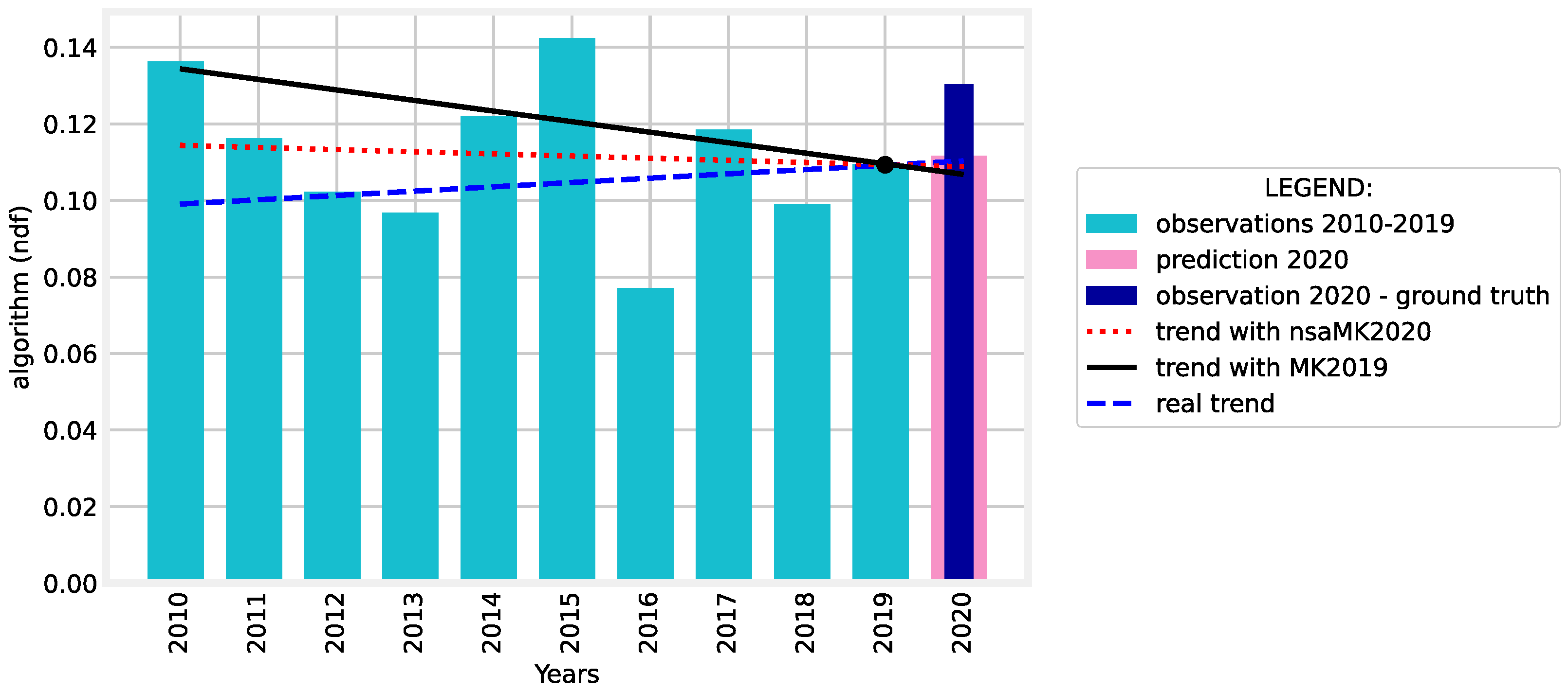
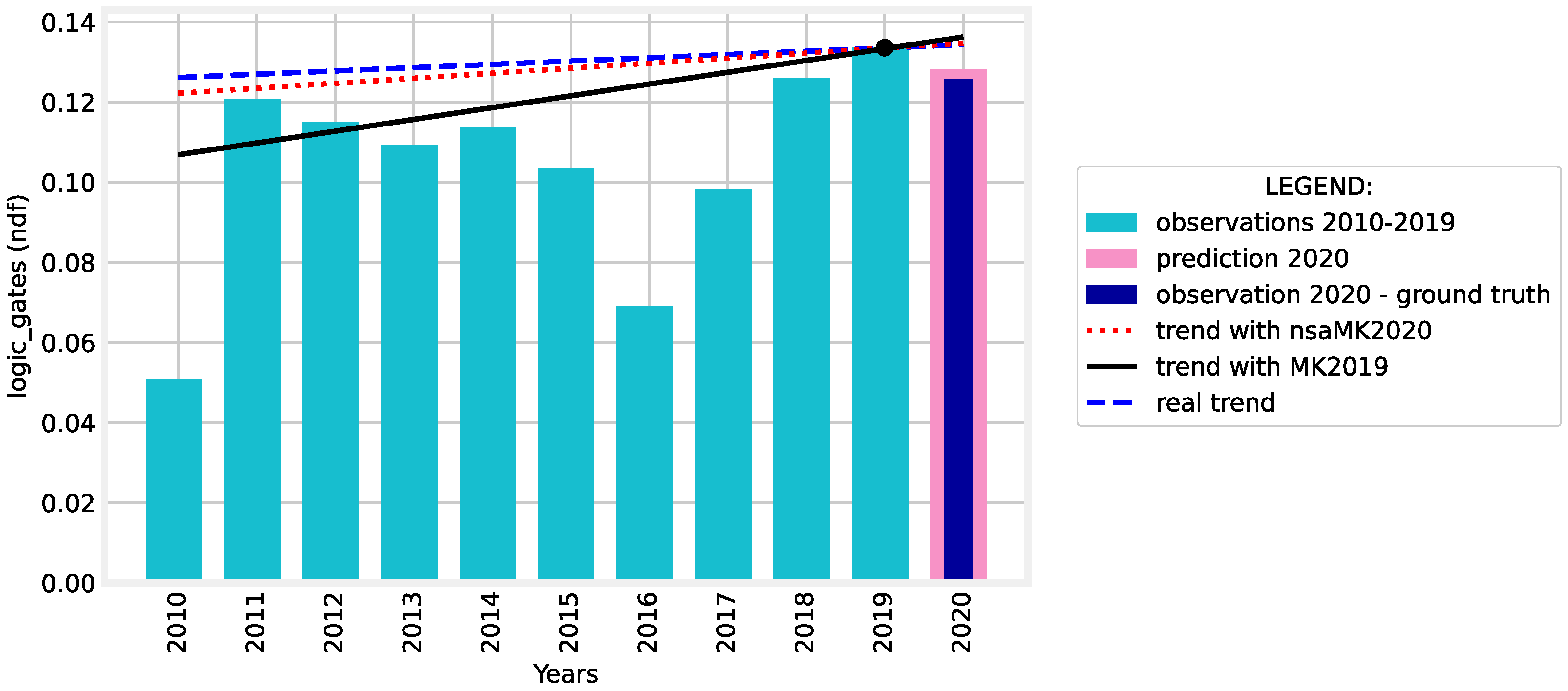
4.2. nsaMK Method Evaluation

In order to compare our nsaMK method with the traditional MK method, we compute z-score, p-value, and Sen’s slope for each of the three hundred EDA terms, considering the corresponding $ndf$ values for ten consecutive years, in three cases:

• Using the Yue and Wang variant of MK test for journal papers published between 2011 and 2020 (MK2020). The results of the MK2020 are considered as ground-truth.
• Using our nsaMK method when considering journal papers published between 2010 and 2019 and the predicted values for 2020 (nsaMK2020).
• Using the Yue and Wang variant of MK test for journal papers published between 2010 and 2019 (MK2019).

By this, the results provided by the new method (nsaMK2020) are compared with the ones offered by MK2019, MK2020 being considered as ground truth.

The parameters for the auto-ARIMA procedure were chosen as follows: the autoregressive order $p\in \{1,2,3\}$, the moving average order $q\in \{0,1,2\}$, and the differencing order $d\in \{0,1,2\}$, while the best ARIMA predictor was automatically selected using the Akaike information criterion described by Equation (8). Since the autoregressive order p cannot be equal to zero, the use of the Yue and Wang variant of the MK test is reasonable.

The obtained results for the top 24 terms in EDA are presented in

Table 2. Comparison results of nsaMK and MK methods for the top 24 terms in EDA.

Term		nsaMK2020			MK2019			MK2020—Ground Truth
		z	p-Value	Slope	z	p-Value	Slope	z	p-Value	Slope
1	integrated circuit	−5.057	$4.2\times {10}^{-7}$	−0.008	−2.715	0.00662	−0.005	−4.809	$1.5\times {10}^{-6}$	−0.008	✓
2	optimization	8.494	0	0.005	5.964	$2.4\times {10}^{-9}$	0.005	10.738	0	0.006	✓
3	computer architecture	4.856	$1.2\times {10}^{-6}$	0.009	4.059	$4.9\times {10}^{-5}$	0.009	6.828	$8.6\times {10}^{-12}$	0.012	✓
4	algorithm	0	1	−0.000	−2.047	0.04060	−0.002	1.061	0.28868	0.001	✓
5	logic gates	0.597	0.54995	0.001	1.257	0.20871	0.002	0.300	0.76357	0.000	✓
6	computational modeling	0.590	0.55509	0.001	−0.522	0.60141	−0.000	1.714	0.08649	0.001	✓
7	latency	1.459	0.14438	0.001	2.027	0.04261	0.001	4.459	$8.2\times {10}^{-6}$	0.004	✓
8	fpga	3.910	$9.2\times {10}^{-5}$	0.006	1.842	0.06533	0.003	3.571	0.00035	0.008	✓
9	task analysis	1.862	0.06250	0	1.816	0.06932	0	2.031	0.04216	0.001	✓
10	energy efficiency	5.235	$1.6\times {10}^{-7}$	0.007	4.005	$6.1\times {10}^{-5}$	0.004	4.894	$9.8\times {10}^{-7}$	0.007	✓
11	machine learning	5.856	$4.7\times {10}^{-9}$	0.003	4.512	$6.3\times {10}^{-6}$	0.003	5.025	$5.0\times {10}^{-7}$	0.005	✓
12	ram	4.346	$1.3\times {10}^{-5}$	0.002	4.232	$2.3\times {10}^{-5}$	0.003	5.118	$3.0\times {10}^{-7}$	0.004
13	neural network	1.938	0.05250	0.002	0.907	0.36428	0	2.892	0.00382	0.004	✓
14	low power	0	1	0.000	1.712	0.08684	0.001	1.910	0.05607	0.001
15	hybrid	3.298	0.00097	0.003	2.580	0.00987	0.002	4.213	$2.5\times {10}^{-5}$	0.004	✓
16	system on chip	3.637	0.00027	0.003	6.111	$9.8\times {10}^{-10}$	0.004	3.694	0.00022	0.003	✓
17	mathematical model	−5.016	$5.2\times {10}^{-7}$	−0.005	−0.924	0.35519	−0.004	−3.686	0.00022	−0.004
18	power	−4.734	$2.1\times {10}^{-6}$	−0.002	−3.678	0.00023	−0.001	−2.532	0.01133	−0.001
19	convolutional neural network	3.842	0.00012	0.001	3.275	0.00105	0.001	3.361	0.00077	0.002	✓
20	logic	0.497	0.61901	0.000	−0.685	0.49291	−0.001	2.419	0.01553	0.001	✓
21	memory management	5.262	$1.4\times {10}^{-7}$	0.003	5.672	$1.4\times {10}^{-8}$	0.003	9.513	0	0.004	✓
22	real time systems	0	1	0	2.307	0.02102	0.002	1.859	0.06289	0.003
23	cmos	7.518	$5.5\times {10}^{-14}$	0.003	7.646	$2.0\times {10}^{-14}$	0.004	6.133	$8.6\times {10}^{-10}$	0.002	✓
24	nonvolatile memory	2.058	0.03958	0.001	2.701	0.00690	0.002	5.340	$9.2\times {10}^{-8}$	0.003

, where, in the last column, we use check marks to label all key terms for which our method achieves superior performance (i.e., the Sen’s slopes offered by nsaMK2020 are closer to the ground truth than the ones provided by MK2019). We may notice that within the top 24 EDA terms in 75% of the cases our method is superior, while on the entire 300 term set this percentage is 66%. Moreover, for the entire set of 300 terms, the mean square error of the Sen’s slopes for our method is 45% better than the one provided by the classic MK method (5.045 × 10${}^{-7}$ vs. 9.041 × 10${}^{-6}$), while for the 24 best ranked EDA terms presented in Table 2, the mean square error is 48% less for our method (2.559 × 10${}^{-6}$ vs. 5.282 × 10${}^{-6}$). When considering only the relevant trends according to p-values (i.e., p-value < 0.01), the results are almost similar: in the 300 terms set, there are 130 terms with identified trends, and for 87 of them (66.9%), our method yields better performance.

In Figure 1 and Figure 2, we present two representative examples, namely for the ’algorithm’ and ’logic gates’ key terms. The light blue observations (i.e., for 2010–2019) are used to compute the slope marked with black solid line by MK2019, the last nine light blue observations, together with the pink-marked auto-ARIMA prediction are used by nsaMK2020 to evaluate the slope presented with red dotted line, and the last nine light blue observations together with the dark blue observation for 2020 are used by MK2020 to reveal the real trend depicted with a blue dashed line (ground truth).

For Figure 1, the best auto-ARIMA prediction for 2020 was obtained when p = 1, d = 0, and q = 1, with an AIC score of −38.633. We may observe that the trend changes from “decreasing” when considering 2010–2019 to “increasing” (ground-truth) and our method nsaMK offers a more appropriate result than MK2019. In the case depicted in Figure 2 the auto-ARIMA obtained the best results when p = 1, d = 0, and q = 0, where the AIC score was −35.658. We may observe that the trend provided with our nsaMK method offers a more suitable result than MK2019.

All methods and experiments were implemented in python 3.8 based on the Mann–Kendall trend test function yue_wang_modification_test() from pyMannKendall 1.4.2 package [32], ARIMA prediction function derived from tsa.statespace.SARIMAX() included in statsmodels 0.13.0 package [33], and CountVectorizer() from scikit-learn 1.0.1 library.

It is worth mentioning that the efficiency of using the nsaMK method strongly depends on the prediction accuracy provided by ARIMA models. In future work, we intend to analyze how the trend evaluation performances change when replacing the ARIMA method in our methodology with exponential smoothing or neural network forecasting. Other limitations of our method are induced by the use of the Mann–Kendall trend test, which has poor results when the time series includes periodicities and tends to provide inconclusive results for short datasets.

5. Conclusions

This paper introduces research publication latency as a new parameter that needs to be considered when evaluating research trends from journal paper metadata, mainly within rapidly evolving scientific fields. The proposed method comprises two steps: (i) a prediction step performed using the auto-ARIMA method to estimate the most recent research evolution that is not yet available in publications; and, (ii) a trend evaluation step using a suitable variant of the Mann–Kendall test with Sen’s slope evaluation. Our simulations, using paper metadata collected from IEEE Transactions on Computer-Aided Design of Integrated Circuits and System, provide convincing results.

References

1. Marrone, M. Application of entity linking to identify research fronts and trends. Scientometrics 2020, 122, 357–379. [Google Scholar] [CrossRef] [Green Version]
2. Hamed, K.H. Trend detection in hydrologic data: The Mann–Kendall trend test under the scaling hypothesis. J. Hydrol. 2008, 349, 350–363. [Google Scholar] [CrossRef]
3. Önöz, B.; Bayazit, M. The power of statistical tests for trend detection. Turk. J. Eng. Environ. Sci. 2003, 27, 247–251. [Google Scholar]
4. Wang, F.; Shao, W.; Yu, H.; Kan, G.; He, X.; Zhang, D.; Ren, M.; Wang, G. Re-evaluation of the power of the mann-kendall test for detecting monotonic trends in hydrometeorological time series. Front. Earth Sci. 2020, 8, 14. [Google Scholar] [CrossRef]
5. Hirsch, R.M.; Slack, J.R. A nonparametric trend test for seasonal data with serial dependence. Water Resour. Res. 1984, 20, 727–732. [Google Scholar] [CrossRef] [Green Version]
6. Marchini, G.S.; Faria, K.V.; Neto, F.L.; Torricelli, F.C.M.; Danilovic, A.; Vicentini, F.C.; Batagello, C.A.; Srougi, M.; Nahas, W.C.; Mazzucchi, E. Understanding urologic scientific publication patterns and general public interests on stone disease: Lessons learned from big data platforms. World J. Urol. 2021, 39, 2767–2773. [Google Scholar] [CrossRef]
7. Sharma, D.; Kumar, B.; Chand, S. A trend analysis of machine learning research with topic models and mann-kendall test. Int. J. Intell. Syst. Appl. 2019, 11, 70–82. [Google Scholar] [CrossRef] [Green Version]
8. Zou, C. Analyzing research trends on drug safety using topic modeling. Expert Opin. Drug Saf. 2018, 17, 629–636. [Google Scholar] [CrossRef]
9. Merz, A.A.; Gutiérrez-Sacristán, A.; Bartz, D.; Williams, N.E.; Ojo, A.; Schaefer, K.M.; Huang, M.; Li, C.Y.; Sandoval, R.S.; Ye, S.; et al. Population attitudes toward contraceptive methods over time on a social media platform. Am. J. Obstet. Gynecol. 2021, 224, 597.e1–597.e4. [Google Scholar] [CrossRef] [PubMed]
10. Chen, X.; Xie, H. A structural topic modeling-based bibliometric study of sentiment analysis literature. Cogn. Comput. 2020, 12, 1097–1129. [Google Scholar] [CrossRef]
11. Chen, X.; Xie, H.; Cheng, G.; Li, Z. A Decade of Sentic Computing: Topic Modeling and Bibliometric Analysis. Cogn. Comput. 2021, 1–24. [Google Scholar] [CrossRef]
12. Zhang, T.; Huang, X. Viral marketing: Influencer marketing pivots in tourism–a case study of meme influencer instigated travel interest surge. Curr. Issues Tour. 2021, 1–8. [Google Scholar] [CrossRef]
13. Chakravorti, D.; Law, K.; Gemmell, J.; Raicu, D. Detecting and characterizing trends in online mental health discussions. In Proceedings of the 2018 IEEE International Conference on Data Mining Workshops (ICDMW), Singapore, 17–20 November 2018; pp. 697–706. [Google Scholar]
14. Modave, F.; Zhao, Y.; Krieger, J.; He, Z.; Guo, Y.; Huo, J.; Prosperi, M.; Bian, J. Understanding perceptions and attitudes in breast cancer discussions on twitter. Stud. Health Technol. Inform. 2019, 264, 1293. [Google Scholar] [PubMed]
15. Neresini, F.; Crabu, S.; Di Buccio, E. Tracking biomedicalization in the media: Public discourses on health and medicine in the UK and Italy, 1984–2017. Soc. Sci. Med. 2019, 243, 112621. [Google Scholar] [CrossRef] [Green Version]
16. King, A.L.O.; Mirza, F.N.; Mirza, H.N.; Yumeen, N.; Lee, V.; Yumeen, S. Factors associated with the American Academy of Dermatology abstract publication: A multivariate analysis. J. Am. Acad. Dermatol. 2021. [Google Scholar] [CrossRef] [PubMed]
17. Andrew, R.M. Towards near real-time, monthly fossil CO2 emissions estimates for the European Union with current-year projections. Atmos. Pollut. Res. 2021, 12, 101229. [Google Scholar] [CrossRef]
18. Box, G.; Jenkins, G.; Reinsel, G. Time-Series Analysis: Forecasting and Control; Holden-Day Inc.: San Francisco, CA, USA, 1970; pp. 575–577. [Google Scholar]
19. Chatfield, C. Time-Series Forecasting; CRC Press: Boca Raton, FL, USA, 2000. [Google Scholar]
20. Whittle, P. Hypothesis Testing in Time-Series Analysis; Almquist and Wiksell: Uppsalla, Sweden, 1951. [Google Scholar]
21. Cryer, J.; Chan, K. Time-Series Analysis with Applications in R; Springer Science & Business Media: New York, NY, USA, 2008. [Google Scholar]
22. Hyndman, R.; Athanasopoulos, G. Forecasting: Principles and Practice; OTexts: Melbourne, Australia, 2018. [Google Scholar]
23. Şen, Z. Innovative Trend Methodologies in Science and Engineering; Springer: New York, NY, USA, 2017. [Google Scholar]
24. Yue, S.; Wang, C. The Mann–Kendall test modified by effective sample size to detect trend in serially correlated hydrological series. Springer Water Resour. Manag. 2004, 18, 201–218. [Google Scholar] [CrossRef]
25. Best, D.; Gipps, P. Algorithm AS 71: The upper tail probabilities of Kendall’s Tau. J. R. Stat. Society. Ser. C (Appl. Stat.) 1974, 23, 98–100. [Google Scholar] [CrossRef]
26. Helsel, D.; Hirsch, R.; Ryberg, K.; Archfield, S.; Gilroy, E. Statistical Methods in Water Resources; Technical Report; US Geological Survey Techniques and Methods, Book 4, Chapter A3; Elsevier: Amsterdam, The Netherlands, 2020; 458p. [Google Scholar]
27. Sen, P.K. Estimates of the regression coefficient based on Kendall’s tau. J. Am. Stat. Assoc. 1968, 63, 1379–1389. [Google Scholar] [CrossRef]
28. Ferragina, P.; Scaiella, U. TagMe: On-the-fly annotation of short text fragments (by Wikipedia entities). In International Conference on Information and Knowledge Management; ACM: Toronto, ON, Canada, 2010; pp. 1625–1628. [Google Scholar]
29. Yosef, M.A.; Hoffart, J.; Bordino, I.; Spaniol, M.; Weikum, G. Aida: An online tool for accurate disambiguation of named entities in text and tables. Proc. VLDB Endow. 2011, 4, 1450–1453. [Google Scholar] [CrossRef]
30. Milne, D.; Witten, I.H. Learning to link with wikipedia. In Proceedings of the 17th ACM conference on Information and knowledge management, Napa Valley, CA, USA, 26–30 October 2008; pp. 509–518. [Google Scholar]
31. Happel, H.J.; Stojanovic, L. Analyzing organizational information gaps. In Proceedings of the 8th Int. Conference on Knowledge Management, Graz, Austria, 3–5 September 2008; pp. 28–36. [Google Scholar]
32. Hussain, M.; Mahmud, I. PyMannKendall: A python package for non parametric Mann–Kendall family of trend tests. J. Open Source Softw. 2019, 4, 1556. [Google Scholar] [CrossRef]
33. Seabold, S.; Perktold, J. Statsmodels: Econometric and statistical modeling with python. In Proceedings of the 9th Python in Science Conference, Austin, TX, USA, 28 June–3 July 2010; pp. 92–96. [Google Scholar]
Figure 1. Trend evaluation comparison for the key term ’algorithm’.
Mathematics 10 00233 g001
Figure 2. Trend evaluation comparison for the key term ’logic gate’.
Mathematics 10 00233 g002