Numerical Studies of Statistical Management Decisions in Conditions of Stochastic Chaos

Abstract

The research presented in this article is dedicated to analyzing the acceptability of traditional techniques of statistical management decision-making in conditions of stochastic chaos. A corresponding example would be asset management at electronic capital markets. This formulation of the problem is typical for a large number of applications in which the managed object interacts with an unstable immersion environment. In particular, this issue arises in problems of managing gas-dynamic and hydrodynamic turbulent flows. We highlight the features of observation series of the managed object’s state immersed in an unstable interaction environment. The fundamental difference between observation series of chaotic processes and probabilistic descriptions of traditional models is demonstrated. We also present an additive observation model with a chaotic system component and non-stationary noise which provides the most adequate characterization of the original observation series. Furthermore, we suggest a method for numerically analyzing the efficiency of conventional statistical solutions in the conditions of stochastic chaos. Based on numerical experiments, we establish that techniques of optimal statistical synthesis do not allow for making effective management decisions in the conditions of stochastic chaos. Finally, we propose several versions of compositional algorithms focused on the adaptation of statistical techniques to the non-deterministic conditions caused by the specifics of chaotic processes.

1. Introduction

A distinctive feature of dynamic open systems that interact with unstable immersion environments is the presence of random perturbations associated with unpredictable physical, economical, political, natural, etc. factors. At each moment of time any given (often latent) factor may start to dominate, which makes many explicitly pronounced local trends appear. The presence of such trends and large areas of observation series that are oscillatory non-periodic processes exactly satisfies the description of chaotic processes [1,2,3,4,5,6]. The chaotic nature of observation series violates the established constraints that are required for statistical estimates to be consistent, efficient, and non-biased. In particular, this refers to the stationarity of the noise, independence of increments, normality (gaussianity) of value variations, and others. The full list of conditions that provide effectiveness and consistency of statistical solutions can be found in classical and modern textbooks on mathematical statistics [7,8,9,10,11,12]. At the same time, as dedicated statistical studies [5,6] show, the most adequate model for describing observation series of the state of unstable objects is an additive combination of a system component consisting of an oscillatory non-periodic process with many local trends, and a random component that is a non-stationary random process. It is obvious that in these conditions, aptly named stochastic chaos, the most important assumption about the repeatability of events which underlies the probabilistic-statistical paradigm has been violated. At the same time, statistical analysis methods remain the primary tool of management decision-making in the conditions of non-determinism. Hence, there is a problem of evaluating the effectiveness of statistical methods of data analysis in conditions in which they are obviously not optimal. Moreover, the estimates made in the conditions of stochastic chaos generally are not unbiased and effective. Therefore, the question about the effectiveness of management decisions based on them remains open. Currently, there are no analytical methods for assessing the quality of statistical estimates generated for chaotic data. The only available assessment means are numerical studies. Therefore, this is the methodology we use in the present article. Note that the specifics of chaotic dynamics do not allow us to obtain a stable result that determines the effectiveness of the estimation procedures themselves. However, considering the management task for which such estimates are made, it would be more sensible to assess the quality of the used algorithms via terminal performance indicators of the constructed strategies. We propose and examine the corresponding technique in this study.

2. Materials and Methods

2.1. Generalized Statistical Decision-Making

Decision-making via statistical synthesis requires constructing a statistical model of the trading situation state. A traditional example of such a model is the statement that an observation series of financial instrument quotations $y_1,y_2,\dots ,y_n$ are independent, identically distributed random variables with a total density $f(y,\theta ),y\in R^1$, where $\theta \in \Theta \subset R^m$ is the set of market parameters, R${}^m$ is an m-dimensional real Euclidean space, and D is the decision space. It is assumed that information about X is needed to select a trading decision $d\in D$ from a predetermined set of management decisions D. In general, d is the result of a certain predictive analysis procedure concerning the trading situation, which includes formalized data processing and interpretation of the obtained results. In practice, a trading decision d is made based on the predicted values of the trading situation state vector $\widehat{X}$.

A trading strategy (a decision function) is a map $S:Y\to D$, i.e., a rule according to which, within the framework of a given statistical model, a set of observations of a trading situation $y_1,y_2,\dots ,y_n\in Y$ corresponds to a trading decision $d\in D$. Thus, a trading strategy is essentially a procedure for analyzing and processing observation series, and a rule for interpreting the result.

The fundamental task of statistical synthesis of management decisions is to choose a strategy that is optimal with respect to some specific quality measure. Such a choice requires the introduction of “more—less”, “better—worse” order relations to the class of all strategies. Strategy $S_0$ is called feasible if it provides management decisions that satisfy a given class of constraints. Strategy $S^{*}$ is optimal in a given class of feasible strategies $S\in \left\{S_0\right\}$ if, taking into account the existing constraints, it outperforms any other strategy from this class by a specified effectiveness measure $\mu \left(S\right)$: $S=S^{*}:\mu \left(S^{*}\right)>\mu \left(S\right),\forall S\in \left\{S_0\right\}$.

The most common method of ordering a set of strategies requires a loss function $w(X,d)$ that maps ${\widehat{X}}_{\tau }\times D\to {\mathbb{R}}^{+}$, where ${\mathbb{R}}^{+}$ is the positive semi-axis of the real axis $\mathbb{R}$, which represents the loss of a trading decision $d\in D$ based on forecast ${\widehat{X}}_{\tau }$ in conditions when the true state of the trading environment is described by a vector parameter $X_{\tau }$, and $\tau$ is the forecasting interval. In estimation problems, the full square of the forecast error is often used as a loss function: $w(X_{\tau },{\widehat{X}}_{\tau })={({\widehat{X}}_{\tau }-X_{\tau })}^2$, i.e., the square of the Euclidean distance between ${\widehat{X}}_{\tau }$ and $X_{\tau }$. Sometimes the loss function is made more complex by adding a weight, thus becoming a weighted sum: $w(X_{\tau },{\widehat{X}}_{\tau })=\lambda \left(X_{\tau }\right){({\widehat{X}}_{\tau }-X_{\tau })}^2$, where the weight $\lambda \left(X_{\tau }\right)$ is selected from the condition of a specific task.

2.2. Specifics of Asset Management in the Conditions of Dynamic Chaos

During the construction of Bayesian management strategies, each acceptable trading strategy $S\in \left\{S_0\right\}$ is mapped to an average loss or risk$R_S\left(X\right)=E\left\{w(X,d)\right\}$, where E is the symbol of mathematical expectation. In the tasks of proactive (i.e., forecast-based) management, which is typical for trading, the main cause of risk is errors in predicting the market situation state vector ${\widehat{X}}_{\tau }$ for the forecast interval $\tau$ chosen by the trader. In the case of a point state vector of a particular financial instrument based on an independent sample of observations $y_1,y_2,\dots ,y_N$ with a distribution density $f\left(Y\right)$, the average loss from the selected trading decision will have the form

$$R_S\left(x_{\tau }\right)=\int \dots {\int }_{R^n}w(x_{\tau },{\widehat{x}}_{\tau }(y_1,\dots ,y_n))\prod _{i=1}^{n}f(y_i\mid x_{\tau })dy.$$

(1)

In the conditions of chaotic dynamics, the observed process does not meet the conditions of stationarity and ergodicity [5,6], the distribution function continuously changes in time and it is not possible to restore it from the previous sample of observations. In this case, the quality of the forecast itself is often estimated based on average square error $R_S=E\left\{{({\widehat{X}}_{\tau }-X_{\tau })}^2\right\}=D\left\{{\widehat{X}}_{\tau }\right\}+{(E\left\{{\widehat{X}}_{\tau }\right\}-X_{\tau })}^2$, where $D\left\{{\widehat{X}}_{\tau }\right\}$ is the variance of the forecast ${\widehat{X}}_{\tau }$. The trading risk from adopting a management strategy S is mainly related to the probabilistic scatter of ${\widehat{X}}_{\tau }$ near the true value $X_{\tau }$ for time $t+\tau$. For a normal distribution law, variance $\underset{n\to \infty }{lim}E\{{\widehat{X}}_{\tau }-X\}=\underset{n\to \infty }{lim}D\left\{{\widehat{X}}_{\tau }\right\}={\sigma }_{\tau }^2$ is a natural scatter measure. However, for chaotic processes, there is no natural general measure of scatter, and the choice has to be made in accordance with the conditions of a specific task.

The risk $R_S\left(X\right)$ associated with the application of strategy S introduces a partial order in the set of strategies so that $S_1\ge S_2\iff R_{S_1}\left(X\right)\le R_{S_2}\left(X\right)$$\forall X\in \left\{X\right\}$.

Generally, in chaotic conditions curves $R_{S_1}\left(X\right)$ and $R_{S_2}\left(X\right)$ intersect and, therefore, the corresponding strategies are generally incomparable. Only in very rare cases there may exist a curve in this class that lies uniformly below all the others at $\forall X\in \left\{X\right\}$, and thus corresponds to the optimal strategy according to the criterion of minimum trading risk.

2.3. Specifics of Applying Statistical Synthesis of Management Strategies in Asset Management

Making control decisions, according to the general theory of statistical decisions, is a procedure for choosing a decision $d\in D_0$ from a set of acceptable decision $D_0$ based on the results of observations of the state of the trading situation of interest to us, described by the process $X_t,t=1,\dots ,n$. In a real situation, this vector process can not always be observed directly and a judgment about it is made on the basis of functionally related, technically accessible observations $Y_t,t=1,\dots ,n$. In other words, an investor or trader usually only has access to direct or indirect observations that are functionally related to the considered trading situation. It would be interesting to consider a generalized representation of an asset’s state phase trajectory in a visual coordinate system “profit P — risk R — state X” using posterior observation data. The trading situation is described by the respective estimates of the specified parameters ${(P,R,X)}_t$ at the time $t=1,\cdots ,n$. In some cases, in particular forecasting changes in the trading situation, the estimated parameters include estimates of the speed and acceleration of changes in the expected profit and risk measures. Then, the vector of the estimated parameters of the phase trajectory at the time $t=1,\cdots ,n$ will have the form ${(P,P^{\prime },P^{″},R,R^{\prime },R^{″},X,X^{\prime },X^{″})}_t$. Observations $Y_t,t=1,\cdots ,n$ are the values of quotation vector of financial instruments $X_t,t=1,\cdots ,n$ and, possibly, some other econometric, political, social and other values, the ensemble of which determines the dynamics of expected changes in profit and risk. The perturbations that a submersion environment exerts on a trading situation ensures that observations contain a random component in all cases. The association between the the parameter vector and observation series $Y_t,t=1,\cdots ,n$ can be expressed with a (generally non-linear) one-dimensional operator: $\Phi :y=\Phi (x,v),$$y\in Y_0$, $x\in X_0$.

A management decision $d\in D$ is chosen based on observations $Y_t,t=1,\cdots ,n$ and all prior information available to the trader. Thus, the procedure for making a management decision, which is the main subject of statistical synthesis, can be written in the form of an operator $S:d=S(Y,x)$. In the ideal case, this operator inverts $\Phi$. The quality of a decision is substantially determined by the availability and reliability of prior information. The lack of reliable prior and current information relating to the trading situation defines the level of uncertainty at which a trading decision is made.

The most complete prior information consists of a probabilistic description of the observation and state spaces that uses a prior distribution of state $g\left(x\right)$ and a family of distributions of observations $f\left(y\right|x)$ for all $x\in X_0$. In this case, the management decision is chosen in accordance with the Bayesian ordering of strategies (1) described above, and the preference rule is based on Bayesian risk

$$R_S(f,g)={\int }_{\Theta }{R}_S(x,f)g\left(x\right)dx={\int }_{X}g\left(x\right){\int }_{R^n}w(x_{\tau },\widehat{x}{}_{\tau }(y_1,\cdots ,y_n))\prod _{i=1}^{n}f(y_i,x)d{y}_i,$$

(2)

where $h\left(x\right)$ is the prior distribution density of the estimated parameter. This approach provides the most effective management decisions for conventional statistical synthesis problems. However, in the conditions of non-stationary dynamics of observation series, prior information turns out to be unsuitable for dynamic reconstruction of distribution functions. The transition to conventional non-Bayesian techniques eliminates the need to restore the prior distribution of the forecast parameter. However, statistical technologies remain inapplicable due to the non-stationarity of the observed process, i.e., the dependence of observation distribution density $f(Y\mid x)$ on time. In particular, maximum likelihood estimation (MLE) [1,2,3,4], which is based on minimization of the joint distribution of observations $L\left(X\right)={\prod }_{i=1}^{n}f(y_i,x)$ and is widely used in statistical synthesis problems [1,2,3,4], turns out to be unsuitable for the same reason — the non-stationarity of observation series.

At the same time, it is known [1,2,3,4,5,6] that the purely random component of observations consisting of the difference between the values of observations, and the smoothed (or system) component of quotation dynamics, will tend to a Gaussian distribution by the central limit theorem. This convergence is approximate, and its degree remains undetermined, due to the impossibility to strictly separate the system component of observation series (deterministic chaos) and the random component.

Nevertheless, even for an approximate Gaussian scheme, using MLE (for a Gaussian model, this leads to the well-known least squares method (LSM)) it is possible to build constructive computational schemes intended to generate predictive management decisions. However, analytical estimates of the quality of such decisions are impossible due to the aforementioned uncertainty regarding the structure of the source data. The only possible way to analyze the problem is thus via numerical studies based on computational experiments. This article is dedicated to the investigation of these issues.

2.4. Observation Model in Asset Management

Figure 1 shows several examples of changes in various currency instrument quotations on a 250-day observation interval.

A visual examination of asset price observation series reveals that their nature is chaotic and can be described by an additive model of form:

$$y_k=x_k+v_k,k=1,\dots ,n,$$

(3)

in which the systemic component of the observed process $x_k,k=1,\cdots ,n$ used to make a decision is an implementation of dynamic chaos [1,2,3,4,5,6,7,8,9,10,13], and usually is an oscillatory non-periodic process with a large quantity of false local trends of undetermined length. The noise $v_k,k=1,\dots ,n$, as shown by applying statistical hypothesis tests [5,6], is a non-stationary heteroscedastic process with a non-degenerate time-dependent autocorrelation function.

Further on, we evaluate the feasibility of using decisions made based on conventional statistical methods in asset management described by the observation model (3). In order to do so, we have constructed a method based on the general theory of evaluating the effectiveness of IT systems presented in [14].

2.5. Analysing the Effectiveness of Statistical Decision-Making in Asset Management

According to the aforementioned theory, the effectiveness of IT systems (in this case, data analysis algorithms) should be assessed according to the performance of the metasystem, in interests of which it is utilized. In the trading case, the management decision is proactive, i.e., it is based on the forecast of the development of the observed process. Conventional statistical synthesis provides an ability to construct an optimal forecast based on well-known methods such as Bayesian estimation, maximum likelihood estimation, least squares method, etc. [1,2,3,4,7], as shown above. It is impossible to analytically estimate whether such methods are effective if the observed processes present chaotic and non-stationary dynamics. Considering that, we present numerical studies based on the terminal estimate of the efficiency of the forecast algorithms and proactive management decisions for real trading asset quotation dynamics processes.

In particular, we consider extrapolation-based computational schemes of optimal statistic forecasting, which estimate the parameters of a polynomial forecast model via the least squares method.

The movement model undergoes statistical identification on the segment of observations that corresponds to the time interval of a financial instrument’s price changing by a specific value $dL$. This approach corresponds to the problem in which the entire range of price changes of a financial instrument is divided into uniform segments of width $dL$. A positive or correct decision based on statistical trend identification accounts for the ability of the considered process to preserve the previously identified trend from the level it was detected at to the crossing of the next level in its direction. In the cases when the process turns around and reaches the opposite level, the respective experiment fragment will be considered to be a false decision. This approach is quite compatible with the tasks of electronic trading, when the gain (TP, Take Profit) is achieved when the process reaches a given level before it reverses and reaches the level of limiting losses (SL, Stop Loss).

Thus, the criterion of decision effectiveness is defined as the estimated probability (frequency) of the process intersecting the trend presence and identification level earlier than the Stop Loss level.

It should be noted that visual posterior observation of chaotic processes reflecting the currency instrument quotation dynamics confirms the assumption that there are local areas with pronounced trends which can be described by low-order polynomials. If this can be proven mathematically, then we can say that the degree of chaos of the observed process decreases locally. This, in turn, opens up prospects for constructing effective trading strategies. Areas that preserve trend direction can be described via conventional statistical methods. If this assumption turns out to be incorrect, it will not be possible to construct effective management strategies based on statistical methods of identifying trends.

As a typical process with non-stationary dynamics, we will consider changes in the quotations of currency pairs at the electronic FOREX market. To study this question, a number of computational experiments for the most commonly used currency instruments are carried out in this paper.

3. Computational Experiments

3.1. Description

The area on which the studied process $Y_t$ changes is divided into equal sectors that are $dL$ points in percentage (pipses) long. Suppose that the process has moved from level $dL$ to the level $L_{k+1}$ above it. We can loosely consider this to be an appearance of a positive trend. Such a transition will be denoted as $L_k\to L_{k+1}$. Conversely, we can understand $L_k\to L_{k-1}$ as negative dynamics [15].

The main problem that we focus on consists in proving the persistence of process $Y_t$ defined as it arriving at the next level of the detected trend.

We assess positive outcome probability, i.e., $Y_t$ going from $L_k\to L_{k+1}$ after it has gone from $L_{k-1}\to L_k$. We define a negative outcome as a opposite transition to the level below $L_k\to L_{k+1}$ directly after an upwards transition $L_{k-1}\to L_k$. Due to symmetry, similar measurements work for downwards transitions as well. Therefore, the set of exhaustive events consists of two positive outcomes $(L_k\to L_{k+1}\mid L_{k-1}\to L_k)$,$(L_k\to L_{k-1}\mid L_{k+1}\to L_k)$ and two negative outcomes $(L_k\to L_{k-1}\mid L_{k-1}\to L_k),(L_k\to L_{k+1}\mid L_{k+1}\to L_k)$.

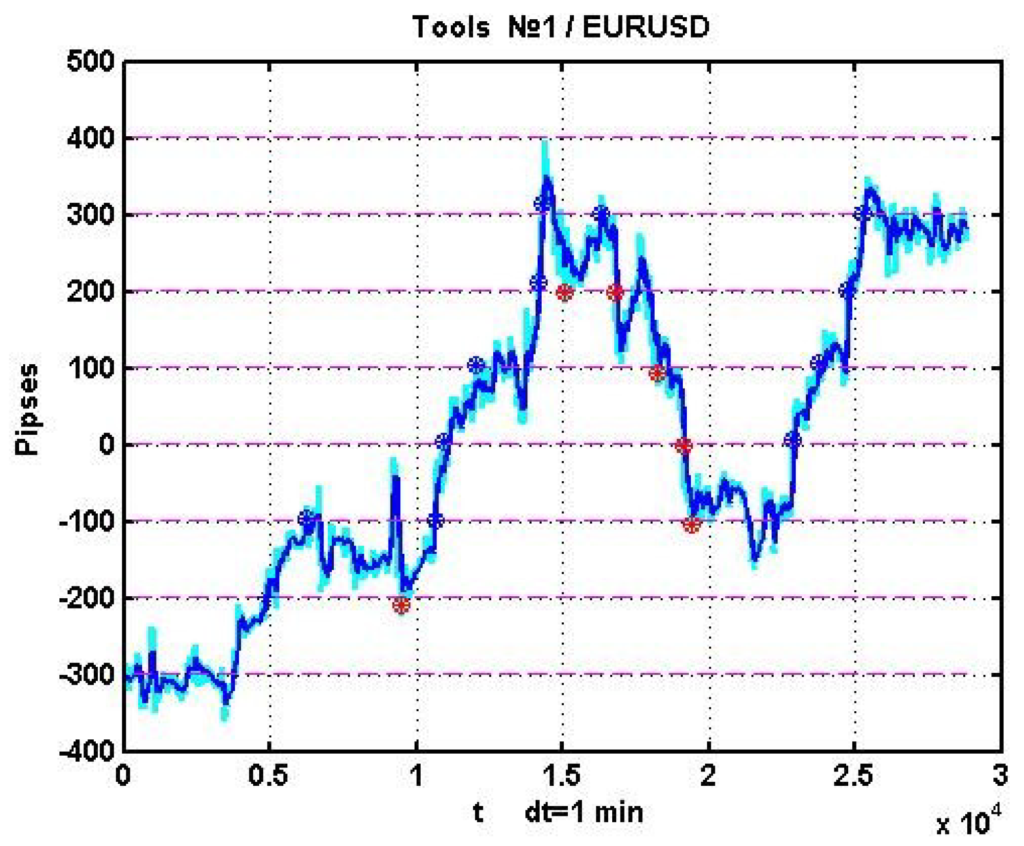
As in illustration, Figure 2 presents an example of EURUSD quotation dynamics on a 10-day observation interval with segmentation boundaries and marks denoting boundary intersections.

The figure presents both the $Y_t,t=1,\cdots ,n$ process and its smoothed version ${\tilde{Y}}_t,t=1,\cdots ,n$. It was smoothed via a simple exponential filter ${\tilde{Y}}_t=\alpha Y_t+\beta {\tilde{Y}}_{t-1},t=1,\dots ,n$, in which $\alpha \in (0,1),\beta =1-\alpha$.

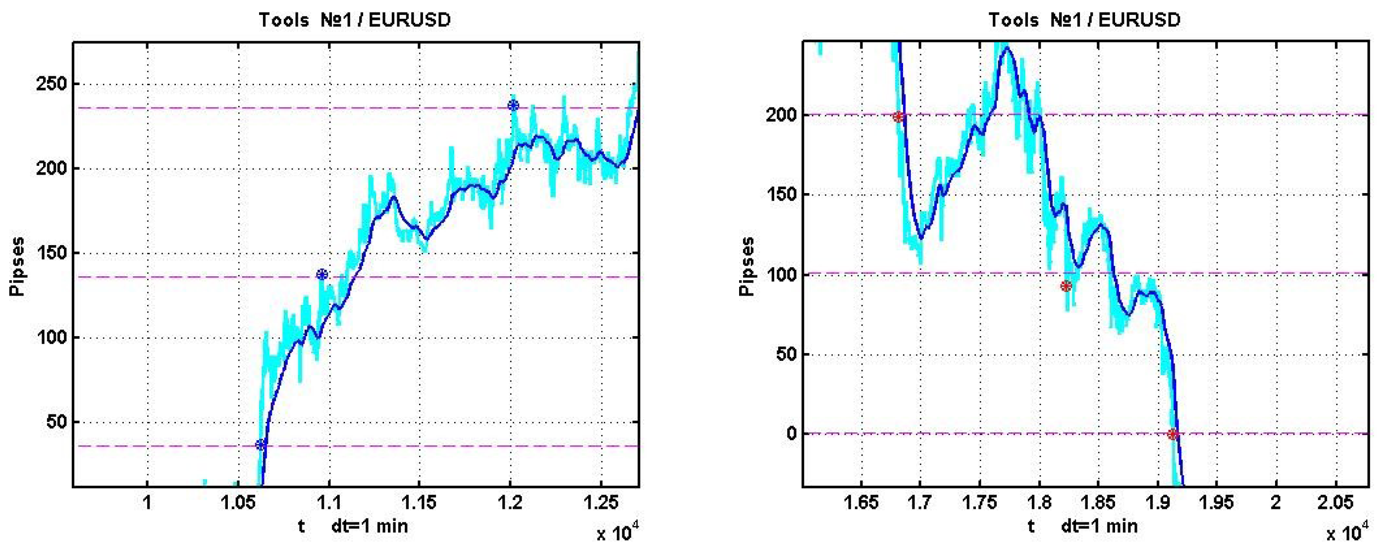
Examples of positive outcomes are shown in Figure 3, and negative ones in Figure 4.

Assume that N experiments were run, each of which has identified a transition from level to level, interpreted as a trend. If this direction persists until the process intersects the next level, this outcome will confirm the trend. Conversely, if the process reverses and reaches the previous level, it will point to trend absence. Suppose that as the result of N consecutive experiments m outcomes prove trend presence, and $N-m$ outcomes disprove it.

Thus, this can be considered as an alternative $H_1:p\ne 0.5$ to the null hypothesis $H_0:p=0.5$ of trend absence, in which $p_n=\frac{m}{n}$ is the frequency of experiments that confirm trend presence. If an experiment is repeated a sufficient number of times, the frequency of observed event is considered to be an estimate of the probability of the corresponding assumption. To test the $H_0$ hypothesis, it is possible to use a well-known rule $u<u^{*}$, where $u=(f_n-0.5){(0.25/n)}^{1/2}$ [8,9,10]. The critical value $u^{*}$ for the right-tailed criterion is found using the Laplace function $\Phi$ table of values, considering that $\Phi \left(u^{*}\right)=\frac{(1-2\gamma )}{2}$. Here, $\gamma$ is the significance level of the null hypothesis.

3.2. Results

In order to cover as many variations of chaotic dynamics in electronic trading as possible, we have considered five 100-day segments for three most widespread financial instruments: EURUSD, EURJPY, and USDJPY. We have used the $dL=100$ (pipses) as the size of the inter-level interval.

Probability is estimated using the frequency of positive outcomes, that is, the ratio of positive outcomes to the total number of experiments. The corresponding results of the computational experiment are presented in

Table 1. Positive outcome frequency at $dL=100$.

Time Interval, Days	EURUSD	EURJPY	USDJPY
1–100	0.552	0.484	0.444
101–200	0.507	0.536	0.465
201–300	0.533	0.552	0.560
301–400	0.494	0.452	0.465
401–500	0.446	0.545	0.444

.

The presented data clearly indicates complete absence of any inertia in quotation dynamics. This statement can be verified with statistical hypothesis testing. As mentioned above, the null hypothesis $H_0:p=0.5$ is tested against the alternative $H_1:p\ne 0.5$.

As an example, consider an experiment for the 100-day interval of EURUSD observation. It resulted in $N=76$ closes, out of which $m=42$ corresponded to the inertia condition at $dL=100$. The relative frequency $\frac{m}{N}=0.552$ corresponds to the value of the decision statistic

$$u=\frac{(\frac{m}{N}-p_0)\sqrt{N}}{\sqrt{p_0{q}_0}}=\frac{0.052\sqrt{76}}{\sqrt{0.25}}=0.91.$$

Here, $q_0=1-p_0,u\in N(0,1)$, i.e., it is subject to the standard Gaussian distribution with the $(0,1)$ parameters. The assumption about the normal distribution of the criterion follows from Laplace’s theorem (for a sufficiently large n, the relative frequency can be approximately considered normally distributed with the mathematical expectation p and standard deviation $\sqrt{\frac{pq}{N}}$). In the general case, this assumption needs additional verification.

The critical area for the symmetrical competing hypothesis $H_1:p\ne 0.5$ is determined based on the selected significance level $\alpha =0.99$. For a two-sided critical area, $u_{cr}$ is determined via the Laplace function value table according to $\Phi \left(u_{cr}\right)=\frac{1-\alpha }{2}=0.005$. Using the distribution tables of the Laplace function, we determine $u_{cr}=2.85$. Therefore, the calculated value of statistic $u=0.91$ belongs to the area of hypothesis acceptance $H_0:p=0.5$, which means that statistical solutions are unsuitable for the considered processes.

The conclusion that inertia is absent in the previous experiment may be caused by an excessively large confirmation interval $dL=100$ p. Let us check whether we can confirm the presence of inertia on smaller segmentation levels. Note that the considered process contains a significant completely random component. Considering the random value spread relatively to the smoothed process from ${\tilde{Y}}_t,t=1,\cdots ,n$$\alpha =0.02$ then its SD on 100-day observation segments oscillates within 11–14 pipses for various currency instruments. Decreasing $\alpha$ to $0.01$, the corresponding SD changes within 15–20 pipses, which is due to a lower degree of smoothness and therefore a smaller difference between the initial and smoothed processes.

The width of the spread is responsible for random decisions that do not correspond to systemic processes of quotation dynamics and therefore skews the conclusions on inertia presence. Thus, in order to obtain a correct conclusion on inertia, the size of the segmentation step (system dynamics) must be significantly larger than the random component.

As an example that illustrates the minimum feasible segmentation step for the presented SD values, consider the same task with $dL=50$. The frequencies of positive outcomes that confirm process inertia can be found in

Table 2. Positive outcome frequency at $dL=50$.

Time Interval, Days	EURUSD	EURJPY	USDJPY
1–100	0.539	0.568	0.522
101–200	0.524	0.528	0.497
201–300	0.529	0.503	0.537
301–400	0.503	0.550	0.534
401–500	0.493	0.548	0.552

.

The results, similarly to the previous case, confirm the stability of the hypothesis $H_0:p=0.5$, which refutes the use of statistical management techniques in a chaotic environment. The positive asymmetry is too small to accept the null hypothesis on the significance of the difference between the frequency of positive outcomes and 50%. The difference between the following series of experiments is that the beginning of each stage of the management process is fixed when the segmentation level is crossed not by the process itself, but by its smoothed version. Positions are closed (i.e., establishing the fact of recognizing or not recognizing inertia in each experiment) by the process $Y_t,t=1,\cdots ,n$ itself.

Obviously, the higher the degree of smoothness, the less the result will depend on the fluctuating component of the process randomly crossing the levels. On the other hand, a higher degree of smoothness inevitably leads to a lag in the smoothed process relative to the original one, which skews the resulting estimates. As a compromise, we will use values $\alpha =0.005-0.02$. The segmentation step, as in the first experiment, is equal to 100 p. The results of estimating the probability of a positive outcome confirming the alternative $H_1$ for five 100-day observation intervals and different values of the exponential filter transfer coefficient $\alpha$ are presented in

Table 3. Positive outcome frequency: opening by smoothed curve.

Time Interval, Days	$\mathit{\alpha }=0.005$	$\mathit{\alpha }=0.01$	$\mathit{\alpha }=0.01$
1–100	0.667	0.681	0.618
101–200	0.771	0.791	0.667
201–300	0.606	0.706	0.612
301–400	0.612	0.653	0.618
401–500	0.648	0.581	0.574

.

It can be seen from the above data that the smoothed version of the process has more inertia, which in general is suitable for making useful trading recommendations. However, one should keep in mind that negative decisions are more drastic in terms of loss, since in this case the dynamics of the quote reverse, and the departure of the process $Y_t,t=1,\cdots ,n$ during the time when the smoothed curve ${\tilde{Y}}_t,t=1,\cdots ,n$ crosses the opening level can be very large.

The final computational experiment is similar to the previous one, but both were carried out by a smoothed process ${\tilde{Y}}_t,t=1,\cdots ,n$ at the intersection of the corresponding level. The results of the experiment are shown in

Table 4. Positive outcome frequency: opening and closing by smoothed curve.

Time Interval, Days	$\mathit{\alpha }=0.005$	$\mathit{\alpha }=0.01$	$\mathit{\alpha }=0.01$
1–100	0.652	0.652	0.593
101–200	0.698	0.706	0.696
201–300	0.686	0.707	0.688
301–400	0.612	0.612	0.582
401–500	0.567	0.534	0.574

.

It is easy to see that the presented results are quite close to the corresponding estimates given in Table 3. In other words, using a smoothed curve did not change the final result. This is due to the fact that the probability of process $Y_t,t=1,\cdots ,n$ reaching the decision level will be higher both with a positive and negative outcome.

The disadvantage of the analysis method proposed above is that it does not take into account the quality of the transitions on which the local trend is detected. For example, transition $Y\left(k\right)\to Y\left(k\right)+dY$ can go on for a long time, with fluctuations and with a large negative “sagging” (it is only necessary that it does not turn around and does not reach level $Y\left(k\right)-dY$). Such a process is quite difficult to perceive as a trend. However, in accordance with the above formalization, such a transition will also be interpreted as a positive trend. In this regard, it makes sense to move on to a more complex trend detection criterion, based, for example, on the average rate of change in the state of the process on a sliding time window of size l:

$$\Delta Y(k,l)=Y(k-l+1,k)=\left[Y\right(k-l+1),Y(k-l+2),\dots ,Y(k\left)\right]$$

(4)

Trend detection in this case is exceeding the value of the linear approximation coefficient $a_1\left(k\right)$ calculated at the observation site $\Delta Y(k,l)$ of a certain critical value $a_1\left(k\right)>a^{*}$. This approach can be generalized to more complex trend detection rules. In particular, we can consider a version of trend detection based on linear approximation coefficients calculated on two observation windows of different lengths $\Delta Y(k,l_1)$ and $\Delta Y(k,l_2)$, $l_1>l_2$, or a version that uses a sliding approximation by a second-order polynomial. The second half of the proposed effectiveness analysis approach, namely, confirming the existence of a trend, remains unchanged. The $H_0$ hypothesis of trend absence in the prolongation of the detected trend means that the process, after its detection at $t_0$, reaches threshold values $Y\left(t_0\right)+dL$ and $Y\left(t_0\right)-dL$ with the same probability, i.e., $H_0:p=p_0=0.5$, p being the value of the observed process at the time of trend detection. An alternative hypothesis indicating the possibility of using such strategies in conditions of market chaos will have the form $H_1:p\ne p_0=0.5$. As in previous experiments, in addition to the main chaotic process $Y\left(t\right)$, we will use its smoothed version $Y_s\left(t\right)$ (4) with a transmission coefficient. The process $Y_s\left(t\right)$, which simulates the system component of chaotic dynamics makes it possible to isolate the purely random component of the initial noise chaotic process $v\left(t\right)=Y\left(t\right)-Y_s\left(t\right)$, which is a centered random process with a distribution that is close to Gaussian. The variance of the residual process $D\left(v\right(t\left)\right)$, in turn, allows us to estimate the lower bound of the parameter $dL$ that determines the level of confirmation or denial of the trend presence hypothesis. The method of conducting computational experiments is close to its prototype described above. An observation series of a trading asset’s state at various non-intersecting 100-day observation intervals is considered as the polygon of chaotic data. Next, we form a sliding observation window $\Delta Y(k,l)$ of size l, on which we calculate approximating polynomials $P(q,l)$, q being their degree. A decision about the presence of a trend is made based on the comparison of estimated coefficients of a with critical values $a^{*}$. The number of outcomes corresponding to the process reaching a predetermined level $dL$ is calculated to statistically verify the effectiveness of management decisions made following trend-based strategies. Due to the symmetry of the task, the negative result consists in a trend reversal and reaching the $-dL$ level. If the ratio of reaching $dL$ to the total number of position openings $m/n$ (the frequency of the event) is close to 0.5, then this confirms the hypothesis $H_0$ that it is impossible to successfully implement trend-based management strategies. The parameters of the computational experiment are observation window l, degree of smoothing polynomial q, threshold values of trends $a^{*}$, and trend confirmation level $dL$. The simplest linear approximation scheme $\tilde{Y}\left(t\right)=a_0+a_{1}t$ is used on a sliding observation window $\Delta Y(k,l)$. A trend is confirmed when the linear approximation coefficient $a_1$ exceeds a pre-set value $a^{*}:a_1\ge a^{*}$. Trend presence is either denied or confirmed when the condition $Y\left(t\right)=Y_0\pm dL$ is met, in which $Y_0=Y\left(t_0\right)$ is the value of the process at the time of trend detection $t_0$, and $dL=30,50,100$ are the trend confirmation levels. The size of the observation window l varies in the (0.1–0.5) day range. A trend is detected if $|a_1|\ge a^{*}$ is satisfied, and confirmed when $Y\left(t\right)=Y_0\pm dL$ levels are reached. Estimates of the probability (frequency) of reaching the trend confirmation level for its various values $dL=25,50,75,100$, for the $l=0.1,0.25,0.5$-day observation window and for threshold values $a^{*}=0.05,0.075,0.1$ on a 100-day observation interval are shown in

Table 5. Trend confirmation frequency for different parameter values.

a${}^{*}$	dL, n l, Days	0.025	0.05	0.075	0.1
0.025	25	0.50	0.48	0.49	0.49
0.025	50	0.51	0.50	0.51	0.50
0.025	75	0.50	0.50	0.50	0.51
0.025	100	0.50	0.51	0.51	0.51
0.05	25	0.50	0.48	0.48	0.50
0.05	50	0.50	0.50	0.51	0.50
0.05	75	0.50	0.50	0.51	0.50
0.05	100	0.50	0.51	0.51	0.51
0.075	25	0.50	0.49	0.49	0.49

.

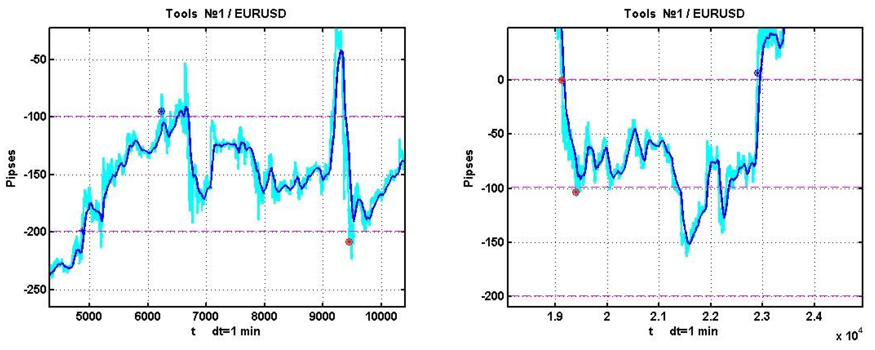
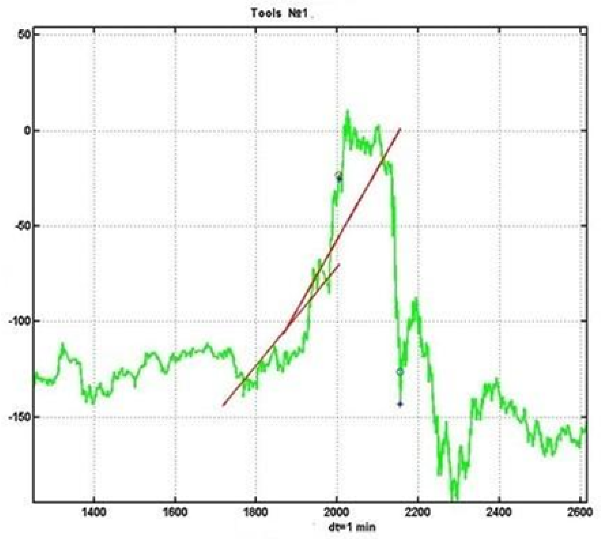
The presented data clearly confirms that it is impossible to successfully prolongate $Y_s\left(t\right)$ in a wide range of changes in intensity values, fixation levels and trend confirmation levels. The disadvantage of this experiment is the fixed length of the sliding observation window l. A large window causes a significant delay in trend detection, which leads to a delayed decision and, as a result, to an incorrect assessment of the probability of trend confirmation. An example is shown in Figure 5.

A small window leads to an increased sensitivity of the trend detection procedure to the random component, which, in turn, leads to statistical errors of Type II (false alarms), that is, to the detection of a non-existent trend. In this regard, it makes sense to consider the problem of trend detection based on a complex criterion that uses two sliding observation windows of different sizes.

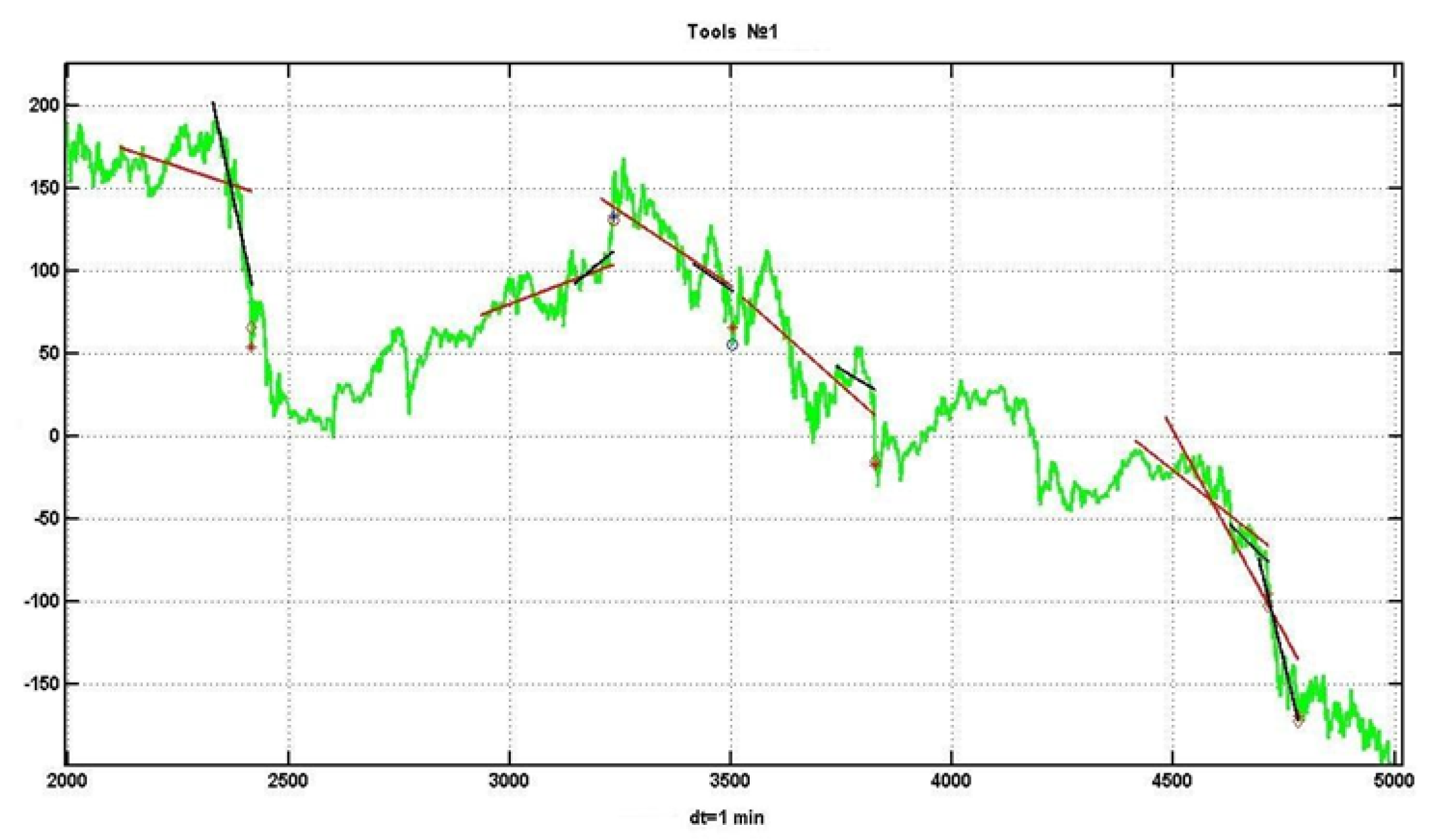
Unlike the previous experiment, in this one we consider two trends. In this case, linear approximations $q=1$ are used for two sliding observation windows of size $l_1$ and $l_2$, $l_1>l_2$. It is obvious that the first trend has stronger smoothing characteristics, and the second is more sensitive to both systemic process changes and “false alarms”. Let $l_1=300$, $l_2=90$ minute counts, critical values of the linear regression coefficient $a_1^{*}=0.05,a_2^{*}=0.1$, the level of trend confirmation $dL=75$. The decision on the presence of a trend is made if both linear regression coefficients exceed their critical values by the absolute value. An example of the implementation of such a scheme is shown in Figure 6.

Longer trends correspond to larger observation windows. Let us consider the result of using this method for four 100-day intervals with different levels of trend confirmation $dL=25:25:100$. The corresponding data is presented in

Table 6. Trend confirmation frequency for various time intervals.

dL, n / $\mathbf{\Delta }\mathit{T}$	1–100 Days	101–200 Days	201–300 Days	301–400 Days
25	0.48	0.49	0.48	0.47
50	0.53	0.46	0.48	0.48
75	0.53	0.50	0.49	0.45
100	0.55	0.50	0.52	0.47

. It is easy to see that the modification did not have a positive effect.

Obviously, the issues of the previous version of this approach have not been resolved. Additionally, the method, as a rule, detects a trend at the time of confirmation (or denial) of the previous trend. At the same time, there is no new trend detection during the confirmation time: this would require a method that simultaneously analyzes several trends. The provided data clearly illustrates the extremely insignificant fluctuations in the frequency of trend confirmation relative to the 0.5 value. This conclusion is easily confirmed by testing the statistical hypothesis $H_0:p=0.5$ about the absence of a trend using U-statistics and confidence level $\alpha =0.99$.

4. Discussion

The applicability of statistical techniques for making management decisions for chaotic processes with a non-stationary random component is a key question in applied problems of asset management. An example of such a problem are effective management strategies based on statistical trend analysis. It is impossible to make analytical estimates of unstable inertia-less system management strategies because the observed processes are unstable parameter-wise. Thus, such studies can be conducted as numerical studies exclusively, considering large observation intervals that cover the variety of stochastic chaos. The technique proposed in the article uses segmentation of the area of change of the considered random process. Thus, it allows us to build a visual system for analyzing the effectiveness of statistical management decisions. The use of the process itself to fix the levels of confirmation or denial of the management effectiveness does not lead to a stable solution due to the high degree of its stochastic spread. The process reaches decision-making levels more often due to high variance than as a result of an inertial trend. This leads to the idea of using a smoothed process for analysing inertia. In particular, good results are obtained with smoothing via an exponential filter with transfer coefficient $\alpha =0.005-0.02$.

A better management result can be expected from more efficient computational schemes for the extraction of the system component in observation series. This issue is currently under study.

Trend analysis that we have conducted does not confirm the effectiveness of trend-based statistical decisions. The trend management strategy for areas with a weak trend of chaotic variations of the immersion environment is essentially non-profitable. Detecting a trend on such segments of price dynamics indicates an upcoming change in the near future and, therefore, it being appropriate to open a position in the opposite direction. In other words, the problem lies not in the statistical methods of estimation themselves, but in the infinite variety of dynamic forms generated by market chaos, which makes it impossible to utilize simple stationary observation models.

It should be noted that currency market inertia is still not confirmed with statistical significance. Some facts that are observed at financial markets confirm this point. If a trend is detected, it is highly likely that in the next moment it will reverse. This means strategies that were effective on backtest could accidentally be effective in the future. The inability of the trend to continue its development can be explained by the fact that most of the time the composition of trading participants is in an equilibrium balance. The influence of trend-following traders (momentum traders) is compensated by market makers and mean reversion traders [16]. At the same time, according to the inaction inertia theory [17], individual investors who missed the opportunity to enter a position at a good price prefer to hold back from a trade at a less favorable price, thereby preventing the trend from developing. However, these factors become insignificant when the fundamental valuation of the asset is changed. When this view is shared by the majority of traders, a continuous trend may develop [18].

This leads to the conclusion that the market situation needs multilateral analysis. In particular, the use of the considered types of statistical solutions combined with an automatic text analyzer, which would assess the general “mood” in relation to the financial instruments used, would significantly increase the effectiveness of the generated decisions.

Therefore, the most promising direction in the development of the task of automatic management of market assets is the development of trading robots based on multi-expert systems. Our current and planned publications will be dedicated to the development of the conceptual and practical aspects of such systems.