Global Stabilization of Nonlinear Finite Dimensional System with Dynamic Controller Governed by 1 − d Heat Equation with Neumann Interconnection

Abstract

This paper deals with the stabilization of a class of uncertain nonlinear ordinary differential equations (ODEs) with a dynamic controller governed by a linear $1-d$ heat partial differential equation (PDE). The control operates at one boundary of the domain of the heat controller, while at the other end of the boundary, a Neumann term is injected into the ODE plant. We achieve the desired global exponential stabilization goal by using a recent infinite-dimensional backstepping design for coupled PDE-ODE systems combined with a high-gain state feedback and domination approach. The stabilization result of the coupled system is established under two main restrictions: the first restriction concerns the particular classical form of our ODE, which contains, in addition to a controllable linear part, a second uncertain nonlinear part verifying a lower triangular linear growth condition. The second restriction concerns the length of the domain of the PDE which is restricted.

1. Introduction

In this work, we deal with the stabilization problem of a chemical reaction by control via heat diffusion equation, where the interaction occurs at the boundary of the heat domain and the control input is located at the second boundary [1,2,3,4]. The closed-loop system of such models is expressed as a nonlinear ODE coupled with $1-d$ heat diffusion systems.

Over the last two decades, the controllability problem of coupled ODE-PDE systems has attracted more and more attention due to their extensive and successful applications in road traffic [5], gas flow pipelines [6], power converters connected to transmission lines [7], and oil drilling [8]. Many problems of stabilization for classes of linear coupled PDE-ODE have been solved, for example, those in [6,9,10,11,12,13], to name just a few. Some nonlinear extensions are studied in [14,15,16], where the nonlinear term is assumed to be globally Lipschitz, and in [17,18,19,20] for general nonlinear ODE.

The controllability theory of linear coupled PDE-ODE systems has been developed in [21]. Since then, many state and output stabilization problems for classes of linear coupled PDE-ODE have been established—those in [6,9,10,11,12,13], to name just a few. Some nonlinear extensions are treated in [14,15,16], where the nonlinear term is assumed to be globally Lipschitz, and in [17,18,19,20] for general nonlinear ODE, where the input-to-state stability (ISS) property is assumed.

For linear ODE systems, by combining predictor feedback and the infinite-dimensional backstepping method, it has been proved that it is possible to compensate the input delays [22,23], diffusive PDE’s [24,25], Schrodinger PDE’s [26], and wave PDEs [27]. For nonlinear ODE systems, results are available for the compensation of transport PDE (or equivalently control delay) [18,23], wave PDE [17,18].

For nonlinear ODE systems, contrary to the control via the wave equation where many results are available, only a few results concerning the stabilization by control through the heat diffusion equation are available. This is mainly due to the fact that the heat propagation is of infinite speed. Recently, the authors of [15] have built a global convergent observer of cascaded nonlinear ODE and heat equation provided that the nonlinear term is globally Lipschitz. It should be noted that the observer design problem studied in [15] is dual to our stabilization problem. More recently, in [2], a global stabilization by heat control was achieved for a class of nonlinear ODEs, where the Lipschitzian global condition of the nonlinear term was rejected and replaced by a domination condition. More recently [4], the rapid stabilization of coupled nonlinear ODE-heat equation was established. The results presented in [2,4] were obtained thanks to a combined technique of high gain feedback and backstepping design for coupled ODE-PDE systems, introduced by [9,24]. Later, in the case where the nonlinear term is dominated by an upper triangular linear system, the observer-based output feedback of the same coupled ODE and $1-d$ heat is designed in [28]. In all the above works, the heat control acts in the ODE equation by Dirichlet interconnection.

In this work, we design a global stabilizing dynamic feedback control governed by the $1-d$ heat equation to stabilize a class of nonlinear ODE systems. The control system acts on the nonlinear ODE plant via a Neumann interconnect. As we shall see, this interconnection poses more difficulties for the study of the coupled system, either in terms of the existence of a solution or in terms of exponential stability.

The remainder of this paper is organized as follows. Section 2 contains the problem reformulation and the state feedback design using the infinite-dimensional backstepping for PDE-ODE coupled systems. Section 3 is devoted to well posedeness of the closed-loop system and to its global exponential stability. Section 4 presents some numerical simulations to illustrate the effectiveness of the proven theoretical results. Section 5 presents the conclusion of this work and some future work directions. Finally, some proofs are collected in Appendix A.

2. Problem Setting and Controller Design

2.1. Problem Formulation

In this paper, we are focused on the design of global stabilizing state feedback for the following class of nonlinear finite-dimensional systems

$$\dot{X}\left(t\right)=AX\left(t\right)+Bv\left(t\right)+f\left(X\left(t\right)\right),$$

(1)

where $X\left(t\right)\in {\mathbb{R}}^n$ is the state, $v\left(t\right)\in \mathbb{R}$ is the input control and matrices $A\in {\mathbb{R}}^{n\times n}$ and $B\in {\mathbb{R}}^{n\times 1}$ are given by

$$A=\left[\begin{array}{ccccc}0& 1& 0& \cdots & 0\\ 0& 0& 1& \ddots & ⋮\\ ⋮& & \ddots & \ddots & 0\\ ⋮& & & \ddots & 1\\ 0& 0& \cdots & \cdots & 0\end{array}\right],B=\left[\begin{array}{c}0\\ ⋮\\ ⋮\\ 0\\ 1\end{array}\right].$$

(2)

System (1) is the well-known perturbed chain of integrators in which $f\left(X\right)$ represents an unknown perturbation. A standard assumption about $f\left(X\right)$ is the following linear triangular domination, which is a sufficient condition for avoiding finite escape time [29].

Assumption A: There exists a known positive constant $\theta$, such that the nonlinear locally Lipschitz function $f\left(X\right)={\left[f_1\left(X\right),\cdots ,f_n\left(X\right)\right]}^T$ satisfies the linear growth rate condition

$$|f_i\left(X\right)|\le \theta \sum _{j=1}^i\left|X_i\right|,$$

(3)

for all $X={[X_1,\cdots ,X_n]}^T\in {\mathbb{R}}^n.$

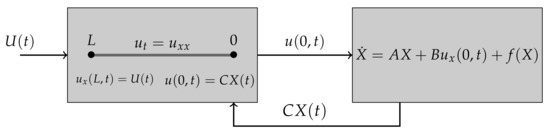
In some practical problems, we are obliged to control a finite-dimensional ODE System (1) by dynamic control law governed by a $1-d$ heat equation (see [1,2]),

$$\begin{array}{ccc}\hfill u_t(x,t)& =& u_{xx}(x,t),x\in (0,L),\hfill \end{array}$$

(4)

$$\begin{array}{ccc}\hfill u(0,t)& =& CX\left(t\right),\hfill \end{array}$$

(5)

$$\begin{array}{ccc}\hfill u_x(L,t)& =& U\left(t\right),\hfill \end{array}$$

(6)

$$\begin{array}{ccc}\hfill v\left(t\right)& =& u_x(0,t)\hfill \end{array}$$

(7)

where $u(·,t)\in L^2(0,L)$ is the state of the control, C is a row matrix in ${\mathbb{R}}^{1\times n}$, $U\left(t\right)\in \mathbb{R}$ is the control input, and $v\left(t\right)\in \mathbb{R}$ is the output of the control system. System (1) in closed loop with dynamic controller (4)–(7) can be written as

$$\begin{array}{cc}\hfill \dot{X}\left(t\right)& =AX\left(t\right)+B{u}_x(0,t)+f\left(X\left(t\right)\right),\hfill \end{array}$$

(8)

$$\begin{array}{cc}\hfill u_t(x,t)& =u_{xx}(x,t),x\in (0,L),\hfill \end{array}$$

(9)

$$\begin{array}{cc}\hfill u(0,t)& =CX\left(t\right),\hfill \end{array}$$

(10)

$$\begin{array}{cc}\hfill u_x(L,t)& =U\left(t\right).\hfill \end{array}$$

(11)

Recent stabilization results for different variants of coupled Systems (8)–(11) (represented by Figure 1) are established in [2,4,28,30]. To the best of our knowledge, this paper is the first to study a coupled system whose ODE subsystem contains a nonlinear term with a Neumann boundary term.

Figure 1. The block diagram of the coupled PDE-ODE system (8)–(11).

To solve the stabilization problem, we apply backstepping transformation for coupled ODE-PDE system introduced recently by [10,12] combined with high gain feedback and domination methods for finite dimensional systems [31].

2.2. Backstepping Transformations

Let $r\ge 1$ be a constant scalar to be designated later, consider the following infinite-dimensional backstepping transformation $\mathcal{F}:(X,u)\to (Z,w)$ as

$$\begin{array}{ccc}\hfill Z\left(t\right)& =& D_{r}X\left(t\right),\hfill \end{array}$$

(12)

$$\begin{array}{ccc}\hfill w(x,t)& =& u(x,t)-{\int }_0^{x}q(x,y)u(y,t)dy-H\left(x\right)D_{r}X\left(t\right),x\in [0,L],\hfill \end{array}$$

(13)

where $q(·,·):[0,L]\times [0,L]\to \mathbb{R}$ and $H(·):[0,L]\to {\mathbb{R}}^{1\times n}$ are two smooth kernels to be selected adequately to reach the stabilization goal. $D_r$ is the following n-order square matrix

$$D_r=diag\left(1,\frac{1}{r},\cdots ,\frac{1}{r^{n-1}}\right).$$

Exploiting the controllability property of the pair $(A,B)$, consider an $1\times n$-matrix $K=[k_1{k}_2\cdots k_n]$, such that $A+BK$ is Hurwitz. The backstepping method aims to determine kernels $q(x,y)$ and $H\left(x\right)$ such that System (8)–(11) is converted by the transformation (12)–(13) to the new nonlinear target system

$$\begin{array}{cc}\hfill \dot{Z}\left(t\right)& =r(A+BK)Z\left(t\right)+r^{-(n-1)}B{w}_x(0,t)+f_r\left(Z\left(t\right)\right),\hfill \end{array}$$

(14)

$$\begin{array}{cc}\hfill w_t(x,t)& =w_{xx}(x,t)+g_r(x,Z\left(t\right)),x\in (0,L)\hfill \end{array}$$

(15)

$$\begin{array}{cc}\hfill w(0,t)& =0,\hfill \end{array}$$

(16)

$$\begin{array}{cc}\hfill w_x(L,t)& =0,\hfill \end{array}$$

(17)

where $g_r(x,Z)$ is a nonlinear term that will be fixed in the sequel. As underlined in the recent papers [2,4], it should be noted that the presence of the term $g_r(x,Z)$ in the subsystem (15) is the main difficulty to establish global exponential stability of the target System (14)–(17).

Let us define the following $2n\times 2n$-matrix

$$\mathcal{A}=\left[\begin{array}{cc}0& rA\\ I& -r^{1-n}BC{D}_r^{-1}\end{array}\right].$$

Proposition 1.

The backstepping transformation (12)–(13) with the following kernels

$$H\left(x\right)=[C{D}_r^{-1},r^{n}K-r^{1-n}C{D}_r^{-1}BC{D}_r^{-1}]e^{x\mathcal{A}}\left[\begin{array}{c}{I}_n\\ O\end{array}\right]$$

(18)

and

$$q(x,y)=r^{1-n}[C{D}_r^{-1},r^{n}K-r^{1-n}C{D}_r^{-1}BC{D}_r^{-1}]e^{(x-y)\mathcal{A}}\left[\begin{array}{c}{I}_n\\ O\end{array}\right]B,$$

(19)

convert the original System (8)–(11) to the following target system

$$\begin{array}{cc}\hfill \dot{Z}\left(t\right)& =r\left(A+BK\right)Z\left(t\right)+r^{1-n}B{w}_x(0,t)+f_r\left(Z\left(t\right)\right),\hfill \end{array}$$

(20)

$$\begin{array}{cc}\hfill w_t(x,t)& =w_{xx}(x,t)-H\left(x\right)f_r\left(Z\left(t\right)\right),x\in (0,L)\hfill \end{array}$$

(21)

$$\begin{array}{cc}\hfill w(0,t)& =0,\hfill \end{array}$$

(22)

$$\begin{array}{cc}\hfill w_x(L,t)& =0,\hfill \end{array}$$

(23)

for the state feedback control

$$\begin{array}{ccc}\hfill U\left(t\right)& =& r^{1-n}C{D}_r^{-1}Bu(L,t)+{\int }_0^L{q}_x(L,y)u(y,t)dy+H^{\prime }\left(L\right)D_{r}X\left(t\right).\hfill \end{array}$$

(24)

The details of transformations and computations are given in Appendix A at the end of the manuscript, and are based on the classical infinite-dimensional backstepping design for coupled PDE-ODE systems as in [9,24].

As mentioned above, due to the presence of the nonlinear term $H\left(x\right)f_r\left(X\right)$ in the subsystem (21), establishing the global exponential stability of the target system is not an easy task. We show that, by selecting the scalar gain r large enough and making a restriction on L (as in [2,15]), it is possible to obtain the desired global exponential stability result.

3. Analysis of the Closed-Loop

In this section, we present the central result of this work which establishes that the System (8)–(11) can be exponentially stabilized by state feedback (24). Specifically, we show that if Assumption A is satisfied, we can select an r that is sufficiently large and a sufficiently small L such that the state feedback (24) globally exponentially stabilizes the System (8)–(11). A precise justification for the restriction of L is provided in the next section.

In the following section, we prove that the System (8)–(11) in closed loop with state feedback (24) is well posed.

3.1. Well-Posedness

Let us define the Hilbert space $\mathcal{H}={\mathbb{R}}^n\times L^2(0,L)$ equipped with its canonical product norm

$${\parallel (X,u)\parallel }_{\mathcal{H}}^2={\left|X\right|}^2+{\parallel u\parallel }^2,$$

where $\parallel .\parallel$ is the canonical $L^2(0,L)$ norm and where $|.|$ denotes the Euclidean norm of ${\mathbb{R}}^n$.

First, considering transformations (12) and (13), it is easy to obtain the following inequalities

$$\begin{array}{cccc}\hfill {\parallel w\parallel }^2& \le a_1{\parallel u\parallel }^2+b_1{\left|X\right|}^2,\hfill & \hfill {\left|Z\right|}^2& \le {\left|X\right|}^2,\hfill \end{array}$$

(25)

where $a_1=3\left(1+{\parallel q\parallel }^2\right),$ and $b_1=3{\parallel H\parallel }^2$. This implies that the operator $\mathcal{F}$ defined by (12)–(13) is continuous. In addition, $\mathcal{F}$ is invertible (see [2] and references therein), and ${\mathcal{F}}^{-1}$ has the following form

$$\begin{array}{ccc}\hfill X\left(t\right)& =& D_r^{-1}Z\left(t\right),\hfill \end{array}$$

(26)

$$\begin{array}{ccc}\hfill u(x,t)& =& w(x,t)+{\int }_0^x{q}_1(x,y)w(y,t)dy+H_1\left(x\right)D_r^{-1}Z\left(t\right),x\in [0,L],\hfill \end{array}$$

(27)

for some kernels $q_1(·,·):[0,L]\times [0,L]\to \mathbb{R}$ and $H_1(·):[0,L]\to {\mathbb{R}}^{1\times n}$ satisfying classical differential equations [9,11]. For System (8)–(11) to be well posed intiially, it is necessary that System (20)–(23) is well posed and that the transformation ${\mathcal{F}}^{-1}$ is continuous. We have the following inequalities that arise from (26) and (27)

$$\begin{array}{ccc}\hfill {\parallel u\parallel }^2\le a_2{\parallel w\parallel }^2+b_2{\left|X\right|}^2,\hspace{1em}\hspace{1em}& \hfill {\left|X\right|}^2& \le r^{2(n-1)}{\left|Z\right|}^2,\hfill \end{array}$$

(28)

where $a_2=3\left(1+\parallel q_1{\parallel }^2\right)$ and $b_2=3r^{2(n-1)}{\parallel H_1\parallel }^2,$ and the continuity of ${\mathcal{F}}^{-1}$ ensues. In the following proposition, we establish that the target, System (20)–(23), is well posed.

We define the operator $\mathcal{A}:\mathcal{D}\left(\mathcal{A}\right)\to \mathcal{H}$ by

$$\begin{array}{cc}\hfill \mathcal{A}\mathcal{Z}& =\left(r(A+BK)Z+r^{1-n}B{w}^{\prime }\left(0\right),w^{″}\right)\hfill \end{array}$$

(29)

with domain $\mathcal{D}\left(\mathcal{A}\right)$ defined by

$$\mathcal{D}\left(\mathcal{A}\right)=\left\{\left(Z,w\right)\in {\mathbb{R}}^n\times H^2(0,L),w\left(0\right)=w^{\prime }\left(L\right)=0\right\}.$$

(30)

Consider the locally Lipschitz nonlinear functional $F:\mathcal{H}\to \mathcal{H}$ defined by $F\left(Z,w\right)=\left(f_r\left(Z\right),-H\left(x\right)f_r\left(Z\right)\right)$. The target, System (20) and (21), is then written in the following abstract form

$$\begin{array}{cc}\hfill \dot{\mathcal{Z}}\left(t\right)& =\mathcal{A}\mathcal{Z}\left(t\right)+F\left(\mathcal{Z}\left(t\right)\right),\hfill \end{array}$$

(31)

where $\mathcal{Z}=\left(Z,w\right)$. The following proposition guarantees the existence and uniqueness of a mild solution for System (31), which is equivalent to the target System (20)–(23).

Proposition 2.

For all initial conditions $\left(Z_0,w_0\right)\in \mathcal{H}$, there exists a unique local mild solution of the target System (20)–(23) defined on a maximal interval $[0,T_{max})$, for some positive time $T_{max}$, and it satisfies

$$\left(Z(·),w(x,·)\right)\in C\left([0,T_{max}),\mathcal{H}\right).$$

Furthermore, if the initial condition $\left(Z_0,w_0\right)$ is in the dense domain, the corresponding local mild solution is a classical solution that satisfies

$$\left(Z(·),w(x,·)\right)\in C^1\left([0,T_{max}),\mathcal{H}\right)\cap C\left([0,T_{max}),\mathcal{D}\left(\mathcal{A}\right)\right).$$

Proof. 

First, we start by showing in the following lemma that operator $\mathcal{A}$ is invertible and that its inverse ${\mathcal{A}}^{-1}$ is compact on $\mathcal{H}$. The proof of the Lemma is given in the Appendix A. □

Lemma 1.

Let $\mathcal{A}$ be defined by (29) and (30). Then, $\mathcal{A}$ is invertible and ${\mathcal{A}}^{-1}$ is compact on $\mathcal{H}$. Hence, $\sigma \left(\mathcal{A}\right)$, the spectrum of $\mathcal{A}$, consists of isolated eigenvalues only.

Now, we consider the eigenvalue problem of $\mathcal{A}$. Solving $\mathcal{A}(Z,w)=\lambda (Z,w)$, where $(Z,w)\in \mathcal{D}\left(\mathcal{A}\right)$ and $\lambda \in \mathbb{C}$. This gives

$$\begin{array}{cc}\hfill r(A+BK)Z+r^{1-n}B{w}^{\prime }\left(0\right)& =\lambda Z,\hfill \end{array}$$

(32)

$$\begin{array}{cc}\hfill w^{″}& =\lambda w,\hfill \end{array}$$

(33)

$$\begin{array}{cc}\hfill w\left(0\right)& =0,\hfill \end{array}$$

(34)

$$\begin{array}{cc}\hfill w^{\prime }\left(L\right)& =0.\hfill \end{array}$$

(35)

By integrating the second-order ODE (33), and taking in account (34), we obtain

$$w\left(x\right)=\alpha \left(e^{-\sqrt{\lambda }x}-e^{\sqrt{\lambda }x}\right),\forall x\in [0,L].$$

(36)

where $\alpha \in \mathbb{C}$. Combining (35) and (36), it yields

$$\sqrt{\lambda }\left(e^{-\sqrt{\lambda }L}+e^{\sqrt{\lambda }L}\right)=0.$$

(37)

Note that, from (37) and the fact that $\mathcal{A}$ is invertible, we obtain $e^{2\sqrt{\lambda }L}=-1=e^{i\pi }$, which gives

$$2\sqrt{\lambda }L=i\pi +2ik\pi ,k\in \mathbb{Z}.$$

Consequently, we can see that the eigenvalues of the operator $\mathcal{A}$ are given by

$${\lambda }_k=-{\pi }^2\frac{{(2k+1)}^2}{4L^2},k\in \mathbb{N},$$

(38)

and the corresponding eigenvectors are given by

$$w_k\left(x\right)=sin\left((2k+1)\frac{\pi x}{L}\right),x\in [0,L].$$

Using (32), it follows that

$$\left((A+BK)-{\lambda }_k{r}^{-1}I\right)Z=-\frac{r^{-n}(2k+1)\pi }{L}B.$$

(39)

Because $(A,B)$ is controllable, without losing generality, it is possible to select matrix K such that $-1$ is the only eigenvalue of $A+BK$. It follows that, if $r\ne {\lambda }_k$, for all $k\in \mathbb{N}$, the matrix $(A+BK)-{\lambda }_k{r}^{-1}I$ is invertible. Then, Equation (39) has the following unique solution

$$\begin{array}{ccc}\hfill Z_k& =& -\frac{r^{-n}{\lambda }_k^{-1}(2k+1)\pi }{L}{\left({\lambda }_k^{-1}(A+BK)-r^{-1}I\right)}^{-1}B.\hfill \end{array}$$

Now, to apply Bari’s Theorem (see [32], Theorem 2.3, p. 317), let $e_1=(1,0,\cdots ,0),e_2=(0,1,0,\cdots ,0),\cdots ,e_n=(0,\cdots ,0,1)$ the canonical basis of the Euclidian space ${\mathbb{R}}^n$ and ${\mathcal{E}}_1=(e_1,0),\cdots ,{\mathcal{E}}_n=(e_n,0),{\mathcal{F}}_k=(0,w_k(.)),k\in \mathbb{N}$ are vectors from $\mathcal{H}$. Then, $\{{\mathcal{E}}_1,\cdots ,{\mathcal{E}}_n,{\mathcal{F}}_k,k\in \mathbb{N}\}$ forms an orthogonal Riesz basis for $\mathcal{H}$. For all $k\in \mathbb{N}$, let ${\mathcal{Z}}_k=(Z_k,w_k(.))$ the eigenvectors of operator $\mathcal{A}$ associated to the eigenvalue ${\lambda }_k$. Because $|Z_k{|}^2=O\left(k^{-2}\right)$, it is assumed that there exists a sufficiently large positive integer N, such that

$$\sum _{k>N}{\parallel {\mathcal{F}}_k-{\mathcal{Z}}_k\parallel }_{\mathcal{H}}^2=\sum _{k>N}O\left(k^{-2}\right)<\infty .$$

Then, according to Bari’s theorem, there exists a Riesz basis $\{{\mathcal{Z}}_k,k\in \mathbb{N}\}$ formed by a set of eigenvectors of operator $\mathcal{A}$. Therefore, $\mathcal{A}$ generates a $C_0$-semigroup on $\mathcal{H}$.

Furthermore, as the function $F\left(\mathcal{Z}\right)$ is locally Lipschitz, it follows by [33] (Theorem 1.4, pp. 185–186), that for all initial condition ${\mathcal{Z}}_0=\left(Z_0,w_0\right)\in \mathcal{H}$, System (31) has a unique local mild solution $\mathcal{Z}\left(t\right)=\left(Z\left(t\right),w(x,t)\right)$ defined in a maximal interval $[0,T_{max})$, for some positive time $T_{max}$. Moreover, if the initial condition ${\mathcal{Z}}_0=\left(Z_0,w_0\right)$ is in the domain $\mathcal{D}\left(\mathcal{A}\right)$, then the corresponding mild solution is a classical solution. Thus, the proof of this proposition is complete.

3.2. Exponential Stability

At this stage, we present and prove our main result concerning the exponential stabilization of the System (1) by dynamic $1-d$ heat control (4)–(7) with feedback (24) and kernels (18) and (19). This is summarized in the following Theorem.

Theorem 1.

Assume that Assumption A is satisfied. Then, there exists a gain matrix K and scalar gain$r^{*}>0$and$L^{*}>0$, such that, for all$0<L\le L^{*}$and$r\ge r^{*},r\ne {\lambda }_k,k=0,1,\cdots$, the dynamic control (4)–(7) with state feedback (24) and kernels$q(x,y),H\left(x\right)$defined in (18) and (19), globally and exponentially stabilizes System (1) in the sense of the norm${\parallel .\parallel }_{\mathcal{H}}$. That is, for all initial condition$(X_0,u_0)\in {\mathbb{R}}^n\times H^2(0,L)$, System (1) in closed loop with dynamic$1-d$heat control (4)–(7) and state feedback (24) has a unique global classical solution,

$$(X(.),u(.,.))\in C^1\left([0,+\infty ),{\mathbb{R}}^n\right)\times C^1\left([0,+\infty ),H^2(0,L)\right).$$

Furthermore, for all$t\ge 0$,

$$\parallel \left(X\left(t\right),u(.,t)\right){\parallel }_{\mathcal{H}}\le C_1{\parallel \left(X_0,u_0\right)\parallel }_{\mathcal{H}}{e}^{-C_{2}t},$$

(40)

where$C_1$and$C_2$are two positive constants.

Before proceeding with the proof of the Theorem, we state the following remark about the restriction on the length L of the heat control domain.

Remark 1.

Note that, for all positive$r^{*}$, it is always possible to find$r\ge r^{*}$and satisfy the condition$r\ne {\lambda }_k,$for all$k=0,1,\cdots$, due to the fact that$|{\lambda }_{k+1}-{\lambda }_k|\ge |{\lambda }_1-{\lambda }_0|=\frac{2{\pi }^2}{L^2}.$

Remark 2.

Note that the imposed restriction on the length L of the heat dynamic control, which must be chosen in some interval$(0,L^{*})$, is reasonable. In fact, on the one hand, the L parameter is part of the dynamic control, and so we can take some restrictions on it, although in practice, it may impose some practical limitations in certain cases.

On the other hand, faced with the presence of an uncertain linear component in the nonlinear part$F\left(\mathcal{Z}\right)$of the System (31), we are forced to take restrictions on the linear part$\dot{\mathcal{Z}}\left(t\right)=\mathcal{A}\mathcal{Z}\left(t\right)$of the nominal system to cover the effect of this uncertain component to maintain the local stability of the entire system. More precisely, the eigenvalues of the unbounded operator$\mathcal{A}$, which are given in (39), are negative, and the greatest value${\lambda }_0=-{\pi }^2/\left(4L^2\right)$tends to zero as L approaches infinity. Hence, the linear uncertain part can destroy the local stability of System (31). Therefore, we prevent zero from going to 0 when L tends to infinity by adopting the restriction${\lambda }_0<-c$, which is equivalent to$L<L^{*}=\pi /\left(2\sqrt{c}\right)$, where c denotes a positive constant.

Proof of Theorem 1.

Let $r\ge 1$ be a positive constant and $r\ne {\lambda }_k,\forall k\in \mathbb{N}$. Because the pair $(A,B)$ is controllable, we select K such that $-1$ is the only eigenvalue of $A+BK$. Then, there exists a positive definite $n\times n$ matrix P, and a positive constant a satisfying the Lyapunov inequality:

$$P(A+BK)+{(A+BK)}^{T}P\le -aI.$$

(41)

Let ${\mathcal{Z}}_0=\left(Z_0,w_0\right)\in \mathcal{D}\left(\mathcal{A}\right)$ be an initial condition and $\mathcal{Z}(.)=\left(Z(·),w(x,·)\right)$ is the corresponding local classical solution of the target system (31) defined on its maximal interval $[0,T_{max})$, where $T_{max}>0$. We consider the Lyapunov function

$$V\left(\mathcal{Z}\left(t\right)\right)=Z^T\left(t\right)PZ\left(t\right)+\frac{d_1}{2}{\parallel w(·,t)\parallel }^2+\frac{d_2}{2}{\parallel w_x(·,t)\parallel }^2.$$

(42)

Using (12), (13), (26) and (27), it is straightforward to show that

$$\begin{array}{cc}\hfill {\parallel w\parallel }^2& \le a_1{\parallel u\parallel }^2+b_1{\left|X\right|}^2,\hfill \end{array}$$

(43)

$$\begin{array}{cc}\hfill \parallel w_x{\parallel }^2& \le a_2\parallel u_x{\parallel }^2+b_2{\parallel u\parallel }^2+c_2{\left|X\right|}^2,\hfill \end{array}$$

(44)

$$\begin{array}{cc}\hfill {\parallel u\parallel }^2& \le {\tilde{a}}_1{\parallel w\parallel }^2+{\tilde{b}}_1{\left|Z\right|}^2,\hfill \end{array}$$

(45)

$$\begin{array}{cc}\hfill \parallel u_x{\parallel }^2& \le {\tilde{a}}_2\parallel w_x{\parallel }^2+{\tilde{b}}_2{\parallel w\parallel }^2+{\tilde{c}}_2{\left|Z\right|}^2,\hfill \end{array}$$

(46)

$$\begin{array}{cc}\hfill {\left|Z\right|}^2& \le {\left|X\right|}^2\le r^{2(n-1)}{\left|Z\right|}^2,\hfill \end{array}$$

(47)

where $a_1=3\left(1+{\parallel q\parallel }^2\right),b_1={3\parallel H\parallel }^2,a_2=4,b_2=4\left(\parallel q_x{\parallel }^2+{\int }_0^{L}q{(x,x)}^{2}dx\right),c_2=4{\parallel H^{\prime }\parallel }^2,$ ${\tilde{a}}_1=3(1+\parallel q_1{\parallel }^2),{\tilde{b}}_1=3r^{2(n-1)}{\parallel H_1\parallel }^2,{\tilde{a}}_2=4,{\tilde{b}}_2=3\left(\parallel q_{1x}{\parallel }^2+{\int }_0^L{q}_1{(x,x)}^{2}dx\right)$ and ${\tilde{c}}_2=4{\parallel H_1^{\prime }\parallel }^2$. Then, from (42)–(47), we obtain

$$\begin{array}{cc}\hfill \underline{\nu }\left({\left|X\right|}^2+{\parallel u\parallel }^2+{\parallel u_x\parallel }^2\right)& \le V\left(\mathcal{Z}\right)\le \overline{\nu }\left({\left|X\right|}^2+{\parallel u\parallel }^2+{\parallel u_x\parallel }^2\right),\hfill \end{array}$$

(48)

where $\underline{\nu }$ and $\overline{\nu }$ are positive constants. The derivative of the Lyapunov function $V\left(\mathcal{Z}\right(t\left)\right)$ along the trajectories of the target system (31) is given by:

$$\begin{array}{c}\hfill \begin{array}{cc}\hfill \dot{V}\left(\mathcal{Z}\left(t\right)\right)& \le -{ra\left|Z\right|}^2+2Z^{T}P{f}_r\left(Z\right)+2r^{1-n}{Z}^{T}PB{w}_x(0,t)\hfill \\ \hfill & +d_1{\int }_0^L\left(w_{xx}(y,t)-H\left(y\right)f_r\left(Z\left(t\right)\right)\right)w(y,t)dy\hfill \\ \hfill & +d_2{\int }_0^L\left(w_{xxx}(y,t)-H^{\prime }\left(y\right)f_r\left(Z\left(t\right)\right)\right)w_x(y,t)dy.\hfill \end{array}\end{array}$$

By performing two integrations in parts, it follows that

$$\begin{array}{ccc}\hfill \dot{V}\left(t\right)& \le & -{ra\left|Z\right|}^2+2Z^{T}P{f}_r\left(Z\right)+2r^{1-n}{Z}^{T}PB{w}_x(0,t)-d_1{\parallel w_x(·,t)\parallel }^2\hfill \\ & & -d_1{\int }_0^{L}w(y,t)H\left(y\right)f_r\left(Z\right)dy-d_2{\parallel w_{xx}(·,t)\parallel }^2-d_2{w}_x(0,t)w_{xx}(0,t)\hfill \\ & & -d_2{\int }_0^L{w}_x(y,t)H^{\prime }\left(y\right)f_r\left(Z\right)dy.\hfill \end{array}$$

(49)

We have $w_{xx}(0,t)=0$, for all $t\in [0,T_{max})$. Indeed, from (21), we obtain $w_{xx}(x,t)=w_t(x,t)+H\left(x\right)f_r\left(Z\left(t\right)\right),$ for all $x\in (0,L)$. Because kernel $H(.)$ is continuous at $x=0$ and $w(·,t)\in H^2(0,L)$, followed by the continuity that $w_{xx}(0,t)=w_t(0,t)+H\left(0\right)f_r\left(Z\left(t\right)\right).$ Moreover, $H\left(0\right)=0$ and (22) yield $w_{xx}(0,t)=0$, for all $t\in [0,T_{max})$. Thus, the boundary term $-d_2{w}_x(0,t)w_{xx}(0,t)$ is cancelled from (49). In the following, we estimate the four cross terms on the right-hand side of (49). Concerning the term $f_r\left(Z\left(t\right)\right)$, as in [2], we have $|f_r\left(Z\right)|\le \theta n|Z|$ and it follows that

$$\begin{array}{cc}\hfill 2Z^{T}P{f}_r\left(Z\right)\le & 2n\theta {\lambda }_{max}\left(P\right){\left|Z\right|}^2,\hfill \end{array}$$

(50)

By the Cauchy–Schwartz inequality, it follows

$$\begin{array}{cc}\hfill 2Z^{T}PB{w}_x(0,t)\le & {\lambda }_{max}\left(P\right){\left|Z\right|}^2+w_x^2(0,t).\hfill \end{array}$$

(51)

For the last two cross terms that have integral representations, by the Cauchy–Schwartz and Poincare inequalities, it yields

$$\begin{array}{cc}\hfill -2d_1{\int }_0^{L}w(y,t)H\left(y\right)f_r\left(Z\right)dy\le & 2d_{1}n\theta \parallel H\parallel \left|Z\right|\parallel w(·,t)\parallel ,\hfill \\ \hfill \le & d_1^2{\parallel H\parallel }^2{\parallel w(·,t)\parallel }^2+n^2{\theta }^2{\left|Z\right|}^2,\hfill \\ \hfill \le & 4d_1^2{L}^2{\parallel H\parallel }^2\parallel w_x{(·,t)\parallel }^2+n^2{\theta }^2{\left|Z\right|}^2,\hfill \end{array}$$

(52)

$$\begin{array}{cc}\hfill -2d_2{\int }_0^L{w}_x(y,t)H^{\prime }\left(y\right)f_r\left(Z\right)dy\le & 2d_{2}n\theta \parallel H^{\prime }\parallel \left|Z\right|\parallel w_x(·,t)\parallel ,\hfill \\ \hfill \le & d_2^2\parallel H^{\prime }{\parallel }^2\parallel w_x{(·,t)\parallel }^2+n^2{\theta }^2{\left|Z\right|}^2.\hfill \end{array}$$

(53)

With Agmon’s inequality, it can be proved that the following inequality holds:

$$-\parallel w_{xx}{(·,t)\parallel }^2\le (1+L)L^{-1}{\parallel w_x(·,t)\parallel }^2-w_x^2(0,t).$$

(54)

By virtue of estimations (50)–(54), inequality (49) becomes

$$\begin{array}{ccc}\hfill \dot{V}\left(t\right)& \le & -\left(ra-2n\theta {\lambda }_{max}\left(P\right)-{\lambda }_{max}\left(P\right)-2n^2{\theta }^2\right){\left|Z\right|}^2-\left(d_2-1\right)w_x^2(0,t)\hfill \\ & & -\left(d_1-2d_1^2{L}^2{\parallel H\parallel }^2-d_2^2{\parallel H^{\prime }\parallel }^2-d_2(1+L)L^{-1}\right){\parallel w_x(·,t)\parallel }^2.\hfill \end{array}$$

(55)

Let $d_2\ge 1$ and rewrite (55) as follows

$$\begin{array}{ccc}\hfill \dot{V}\left(t\right)& \le & -c_1{\left(r\right)\left|Z\right|}^2-c_2(d_1,r){\parallel w_x\parallel }^2,\hfill \end{array}$$

(56)

where

$$\begin{array}{cc}\hfill c_1\left(r\right)& =ra-2n\theta {\lambda }_{max}\left(P\right)-{\lambda }_{max}\left(P\right)-2n^2{\theta }^2,\hfill \end{array}$$

(57)

$$\begin{array}{cc}\hfill c_2(d_1,r)& =d_1-2d_1^2{L}^2{\parallel H\parallel }^2-d_2^2{\parallel H^{\prime }\parallel }^2-d_2(1+L)L^{-1}.\hfill \end{array}$$

(58)

In the next step, we choose the parameters $d_1$ and r such that constants $c_1\left(r\right)$ and $c_2(d_1,r)$ are positive. We point out that $\parallel H\parallel$ and $\parallel H^{\prime }\parallel$ depend on the design parameters r and L. For this reason, we use the notations $\parallel H_{r,L}\parallel ,\parallel H_{r,L}^{\prime }\parallel$ instead of $\parallel H\parallel ,\parallel H^{\prime }\parallel$, respectively. Let

$$\begin{array}{cc}\hfill r_1^{*}& =\frac{1}{a}\left(1+2n\theta {\lambda }_{max}\left(P\right)+{\lambda }_{max}\left(P\right)+2n^2{\theta }^2\right).\hfill \end{array}$$

(59)

By choosing $r>r_1^{*}$ (recall that we have imposed $r\ne {\lambda }_k,\forall k\in \mathbb{N}$ to ensure the existence and uniqueness of the classical solution $\mathcal{Z}\left(t\right)$), we obtain $c_1\left(r\right)>0$. Now, we show that we can choose a positive parameter $d_1$, such that $c_2(d_1,r)>0$. Indeed, the discriminant of the second-degree polynomial function $d_1\to c_2(d_1,r)$ is:

$$\Delta \left(L\right)=1-8L\parallel H_{r,L}{\parallel }^2\left(L{d}_2^2{\parallel H_{r,L}^{\prime }\parallel }^2+d_2(1+L)\right).$$

(60)

From (18), it is obvious that there exist two positive constants $\kappa$ and $\omega$ that are independent of the constant L, such that

$$\begin{array}{c}\hfill max\left\{\right|H_{r,L}\left(x\right)|,|H_{r,L}^{\prime }\left(x\right)\left|\right\}\le \kappa e^{\omega x},\forall x\in [0,L].\end{array}$$

(61)

Taking the $L^2(0,L)$-norm in Equation (61), we obtain

$$\begin{array}{c}\hfill max\{\parallel H_{r,L}{\parallel }^2,\parallel H_{r,L}^{\prime }{\parallel }^2\}\le \frac{{\kappa }^2}{2\omega }\left(e^{2\omega L}-1\right).\end{array}$$

(62)

Taking into account (60) and (62), it follows that $\Delta \left(L\right)$ tends to 1, when L towards 0, and then there exists a positive constant $L^{*}$, such that the discriminant $\Delta \left(L\right)>0$, for all $L\in (0,L^{*})$. It follows that, for all $L\in (0,L^{*})$, the polynomial function $d_1\to c_2(d_1,r)$ has the two following positive roots:

$$\begin{array}{cccc}\hfill d_1^{\left(1\right)}& =\frac{1-\sqrt{\Delta \left(L\right)}}{4L^2{\parallel H_{r,L}\parallel }^2},\hfill & \hfill d_1^{\left(2\right)}& =\frac{1+\sqrt{\Delta \left(L\right)}}{4L^2{\parallel H_{r,L}\parallel }^2}.\hfill \end{array}$$

(63)

By choosing $d_1\in (d_1^{\left(1\right)},d_1^{\left(2\right)})$, it yields in $c_2(d_1,r)>0$. In summary, if the parameters $r,d_1$ and L satisfy $r>r_1^{*},r\ne {\lambda }_k,\forall k\in \mathbb{N}$, $d_1\in (d_1^{\left(1\right)},d_1^{\left(2\right)})$ and $L\in (0,L^{*})$, respectively, then using the Poincare inequality, from (56), we obtain

$$\begin{array}{ccc}\hfill \dot{V}\left(\mathcal{Z}\left(t\right)\right)& \le & -c_1\left(r\right){\left|Z\right|}^2-\frac{c_2(d_1,r)}{1+4L^2}\left({\parallel w\parallel }^2+{\parallel w_x\parallel }^2\right).\hfill \end{array}$$

(64)

Then, from (64), it follows that

$$\begin{array}{ccc}\hfill \dot{V}\left(\mathcal{Z}\left(t\right)\right)& \le & -\delta V\left(\mathcal{Z}\right(t\left)\right),\hfill \end{array}$$

(65)

where $\delta =min\left\{c_1\left(r\right),\frac{c_2(d_1,r)}{1+4L^2}\right\}$ is a positive constant. Integrating (65) yields $V\left(\mathcal{Z}\left(t\right)\right)\le V\left(\mathcal{Z}\left(0\right)\right)e^{-\delta t},$ or equivalently

$$\parallel \left(Z\left(t\right),w(.,t)\right){\parallel }_{\mathcal{H}}^2\le \frac{\overline{\nu }}{\underline{\nu }}\parallel \left(Z_0,w_0\right){\parallel }_{\mathcal{H}}^2{e}^{-\delta t},$$

(66)

for all $t\in [0,T_{max})$. Therefore, the local solution $\left(Z\left(t\right),w(·,t)\right)$ of the target system (20)–(23) is bounded on the maximal interval $[0,T_{max})$. Then, $T_{max}=+\infty$ and the solution $\left(Z\left(t\right),w(·,t)\right)$ converges exponentially to the origin. Thus, the closed-loop system (8)–(11) with state feedback (24) has a unique global classical solution $\left(X\right(t),u(x,t)$ defined on $[0,+\infty )$ and converges exponentially to the origin. This completes this proof. □

4. Numerical Example

In this section, we present a numerical simulation for the closed-loop system (8)–(11) to validate the performance of our feedback control. Consider the following numerical system having the same structure as (8)–(11):

$$\begin{array}{ccc}\hfill {\dot{X}}_1\left(t\right)& =& X_2\left(t\right)+f_1\left(X_1\left(t\right)\right),\hfill \end{array}$$

(67)

$$\begin{array}{ccc}\hfill {\dot{X}}_2\left(t\right)& =& u_x(0,t)+f_2(X_1\left(t\right),X_2\left(t\right)),\hfill \end{array}$$

(68)

$$\begin{array}{ccc}\hfill u_t(x,t)& =& u_{xx}(x,t),x\in (0,L),\hfill \end{array}$$

(69)

$$\begin{array}{ccc}\hfill u(0,t)& =& X_1\left(t\right),\hfill \end{array}$$

(70)

$$\begin{array}{ccc}\hfill u_x(L,t)& =& U\left(t\right),\hfill \end{array}$$

(71)

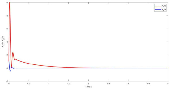
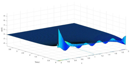
with $C=[1,0],B={[0,1]}^T,$ and $A=\left[\begin{array}{cc}0& 1\\ 0& 0\end{array}\right]$. Let $K=[-1-2]$, for which $-1$ is the only eigenvalue of the matrix $A+BK$. The solution of the Lyapunov Equation (41) is the matrix $P=\left[\begin{array}{cc}1.5& -0.5\\ -0.5& 0.5\end{array}\right]$, its maximal eigenvalue is ${\lambda }_{max}\left(P\right)=1.7071$ and the value of the constant a in the inequality (41) is equal to 1. Let $f_1\left(X_1\right)=0$ and $f_2(X_1,X_2)=0.1sin(X_1+X_2)$. It is easy to verify that the nonlinear function $f\left(X\right)={(f_1\left(X_1\right),f_2(X_1,X_2))}^T$ satisfies the A hypothesis with $\theta =0.1$. Therefore, all assumptions of Theorem 1 are satisfied. The kernels $H\left(x\right),q(x,y)$, and the state feedback $U\left(t\right)$ given, respectively, by (18), (19) and (24) can be computed explicitly. Using (59), it follows that $r_1^{*}=3.4699$. We note that the explicit computation of the optimal value $L^{*}$ of L is hard to determine. For the numerical simulation, we adopt the finite difference scheme directly to discretize System (67)–(71). The steps of space and time are taken as $0.05$ and $0.00125$, respectively. In addition, we take $L=2$ and the initial values of system states are $(X_1\left(0\right),X_2\left(0\right),u_0\left(x\right))=(1,1,cos\left(2\pi x\right))$. As a result, the simulation of the solution is plotted in Figure 2 and Figure 3. Figure 2 displays the state $X\left(t\right)$, while Figure 3 shows the trajectory of the state $u(x,t)$. It can be seen that both the states $X\left(t\right)$ and $u(x,t)$ converge to zero, which indicates that the closed-loop system, System (67)–(71), is exponentially stable.

Figure 2. Trajectory of the state $X\left(t\right)$ solution of System (67)–(71).

Figure 3. Trajectory of the state $u(x,t)$ solution of System (67)–(71).

5. Conclusions

In this paper, we solved the problem of global exponential stabilization for a class of finite-dimensional nonlinear uncertain systems using dynamic $1-d$ heat control. The nonlinear term of the ODE system is dominated by a linear lower-triangular term multiplied by a known parameter. Dynamic control acts in the system plant by Neumann interconnection at the boundary $x=0$ of the heat domain, and the control input is located at the boundary $x=L$. The problem is solved by combining a backstepping design for coupled ODE-PDE systems and high-gain state feedback, and finally, we presented numerical examples to confirm the obtained results. This study leaves some open questions for future works. A very interesting result was established later in [28], which solved the output stabilization problem of a cascaded finite-dimensional nonlinear feedforword system and a $1-d$ heat diffusion system. The method used can be generalized to solve the stabilization problem for a cascaded general nonlinear system coupled with a heat equation as follows:

$$\begin{array}{ccc}\hfill \dot{X}\left(t\right)& =& g\left(X\right(t),u(0,t\left)\right),\hfill \\ \hfill u_t(x,t)& =& u_{xx}(x,t),x\in (0,L),\hfill \\ \hfill u_x(0,t)& =& 0,\hfill \\ \hfill u_x(L,t)& =& U\left(t\right),\hfill \end{array}$$

under some weak assumptions on the nonlinear function $g(.,.)$.

References

- Zhao, A.; Xie, C. Stabilization of coupled linear plant and reaction—Diffusion process. J. Frankl. Inst. 2014, 351, 857–877. [Google Scholar] [CrossRef]
- Benabdallah, A. Stabilization of a class of nonlinear uncertain ordinary differential equation by parabolic partial differential equation controller. Int. J. Robust Nonlinear Control 2020, 30, 3023–3038. [Google Scholar] [CrossRef]
- Zhen, Z.; Si, Y.; Xie, C. Indirect control to stabilize reaction-diffusion equation. Int. J. Control 2021, 94, 3091–3098. [Google Scholar] [CrossRef]
- Benabdallah, A.; Dlala, M. Rapid exponential stabilization by boundary state feedback for a class of coupled nonlinear ODE and 1 − d heat diffusion equation. Discret. Contin. Dyn. 2021. [Google Scholar] [CrossRef]
- Goatin, P. The Aw-Rascle vehicular traffic flow model with phase transitions. Math. Comput. Model. 2006, 44, 287–303. [Google Scholar] [CrossRef]
- Tang, Y.; Prieur, C.; Girard, A. Stability analysis of a singularly perturbed coupled ODE-PDE system. In Proceedings of the 54 th IEEE Conference on Decision and Control, Osaka, Japan, 15–18 December 2015; pp. 4591–4596. [Google Scholar]
- J Daafouz, J.; Tucsnak, M.; Valein, J. Nonlinear control of a coupled PDE-ODE system modeling a switched power converter with a transmission line. Syst. Control Lett. 2014, 70, 92–99. [Google Scholar] [CrossRef]
- Saldivar, B.; Mondié, S.; Avila Vilchis, J.C. The Control of Drilling Vibrations: A Coupled PDE-ODE Modeling Approach. Int. J. Appl. Math. Comput. Sci. 2016, 26, 335–349. [Google Scholar] [CrossRef]
- Tang, S.; Xie, C. State and output feedback boundary control for a coupled PDE-ODE system. Syst. Control Lett. 2011, 60, 540–545. [Google Scholar] [CrossRef]
- Tang, S.; Xie, C. Stabilization for a coupled PDE-ODE control system. J. Frankl. Inst. 2011, 348, 2142–2155. [Google Scholar] [CrossRef]
- Krstic, M. Compensating a String PDE in the Actuation or Sensing Path of an Unstable ODE. IEEE Trans. Autom. Control 2009, 54, 1362–1368. [Google Scholar] [CrossRef]
- Susto, G.A.; Krstic, M. Control of PDE-ODE cascades with Neumann interconnections. J. Frankl. Inst. 2010, 347, 284–314. [Google Scholar] [CrossRef]
- Boundary stabilization of a coupled wave-ODE system with internal anti-damping. Int. J. Control 2012, 85, 1683–1693. [CrossRef]
- Wu, H.N.; Wang, J.W. Observer design and output feedback stabilization for nonlinear multivariable systems with diffusion PDE-governed sensor dynamics. Nonlinear Dyn. 2013, 72, 615–628. [Google Scholar] [CrossRef]
- Ahmed-Ali, T.; Giri, F.; Krstic, M.; Lamnabhi-Lagarrigue, F. Observer design for a class of nonlinear ODE-PDE cascade systems. Syst. Control Lett. 2015, 83, 19–27. [Google Scholar] [CrossRef]
- Cai, X.; Liao, L.; Zhang, J.; Zhang, W. Observer design for a class of nonlinear system in cascade with counter-convecting transport dynamics. Kybernetika 2016, 52, 76–88. [Google Scholar] [CrossRef][Green Version]
- Bekiaris-Liberis, N.; Krstic, M. Compensation of Wave Actuator Dynamics for Nonlinear Systems. IEEE Trans. Autom. Control 2014, 59, 1555–1570. [Google Scholar] [CrossRef]
- Diagne, M.; Bekiaris-Liberis, N.; Otto, A.; Krstic, M. Control of Transport PDE/Nonlinear ODE Cascades with State-Dependent Propagation Speed. In Proceedings of the IEEE 55th Conference on Decision and Control, Las Vegas, NV, USA, 12–14 December 2016; pp. 3125–3130. [Google Scholar]
- Hasana, A.; Aamoa, O.M.; Krstic, M. Boundary observer design for hyperbolic PDE-ODE cascade systems. Automatica 2016, 68, 75–86. [Google Scholar] [CrossRef]
- Cai, X.; Krstic, M. Nonlinear stabilization through wave PDE dynamics with a moving uncontrolled boundary. Automatica 2016, 68, 27–38. [Google Scholar] [CrossRef]
- Zhao, X.; Weiss, G. Controllability and Observability of a Well-posed System Coupled with a Finite-dimensional System. IEEE Trans. Autom. Control 2011, 56, 1–12. [Google Scholar] [CrossRef]
- Jankovic, M. Recursive predictor design for state and output feedback controllers for linear time delay systems. Automatica 2010, 46, 510–517. [Google Scholar] [CrossRef]
- Bekiaris-Liberis, N.; Krstic, M. Compensation of state-dependent input delay for nonlinear systems. IEEE Trans. Autom. Control 2013, 58, 275–289. [Google Scholar] [CrossRef]
- Krstic, M. Compensating actuator and sensor dynamics governed by diffusion PDEs. Syst. Control Lett. 2009, 58, 372–377. [Google Scholar] [CrossRef]
- Bekiaris-Liberis, N.; Krstic, M. Compensating the distributed effect of diffusion and counter-convection in multi-input and multi-output LTI systems. IEEE Trans. Autom. Control 2011, 56, 637–642. [Google Scholar] [CrossRef]
- Ren, B.; Wang, J.M.; Krstic, M. Stabilization of an ODE-Schrodinger Cascade. Syst. Control Lett. 2013, 62, 503–510. [Google Scholar] [CrossRef]
- Bekiaris-Liberis, N.; Krstic, M. Compensating the distributed effect of a wave PDE in the actuation or sensing path of MIMO LTI Systems. Syst. Control Lett. 2010, 59, 713–719. [Google Scholar] [CrossRef]
- Chang, Y.; Sun, T.; Zhang, X.; Chen, X. Output Feedback Stabilization for a Class of Cascade Nonlinear ODE-PDE Systems. Int. J. Control. Autom. Syst. 2021, 19, 2519–2528. [Google Scholar] [CrossRef]
- Mazenc, F.; Praly, L. Global stabilization by output feedback: Examples and counter examples. Syst. Control Lett. 1994, 23, 119–125. [Google Scholar] [CrossRef]
- Liu, X.; Xie, C. Control law in analytic expression of a system coupled by reaction—Diffusion equation. Syst. Control Lett. 2020, 137, 104643. [Google Scholar] [CrossRef]
- Andrieua, V.; Praly, L. A unifying point of view on output feedback designs for global asymptotic stabilization. Automatica 2009, 45, 1789–1798. [Google Scholar] [CrossRef]
- Gohbergue, I.; Krein, M.G. Introduction to the Theory of Linear Nonselfadjoint Operators; American Mathematical Society: Providence, RI, USA, 1969. [Google Scholar]
- Pazy, A. Semigroups of Linear Operators and Applications to Partial Differential Equations; Springer: New York, NY, USA, 1992. [Google Scholar]
- Adams, R.A.; Fournier, J.J.F. Sobolev Spaces, 2nd ed.; Elsevier/Academic Press: Amsterdam, The Netherlands, 2003. [Google Scholar]
Publisher’s Note: MDPI stays neutral with regard to jurisdictional claims in published maps and institutional affiliations. |
© 2022 by the authors. Licensee MDPI, Basel, Switzerland. This article is an open access article distributed under the terms and conditions of the Creative Commons Attribution (CC BY) license (https://creativecommons.org/licenses/by/4.0/).