Article

Forecasting the Hydrogen Demand in China: A System Dynamics Approach

1
Department of Economy and Management, North China Electric Power University, Baoding 102206, China
2
School of Electrical Engineering, Beijing Jiaotong University, Beijing 100091, China
*
Author to whom correspondence should be addressed.
Mathematics 2022, 10(2), 205; https://doi.org/10.3390/math10020205
Submission received: 22 November 2021 / Revised: 6 January 2022 / Accepted: 6 January 2022 / Published: 10 January 2022

Abstract

:
Many countries, including China, have implemented supporting policies to promote the commercialized application of green hydrogen and hydrogen fuel cells. In this study, a system dynamics (SD) model is proposed to study the evolution of hydrogen demand in China from the petroleum refining industry, the synthetic ammonia industry, and the vehicle market. In the model, the impact from the macro-environment, hydrogen fuel supply, and construction of hydrogen facilities is considered to combine in incentives for supporting policies. To further formulate the competitive relationship in the vehicle market, the Lotka–Volterra (LV) approach is adopted. The model is verified using published data from 2003 to 2017. The model is also used to forecast China’s hydrogen demand up to the year of 2030 under three different scenarios. Finally, some forward-looking guidance is provided to policy makers according to the forecasting results.

1. Introduction

Hydrogen is a type of zero-carbon and high-efficiency energy under serious consideration for many countries’ low-carbon transport, industrial decarbonization, and heat provisions [1]. Hydrogen is widely used to produce synthetic ammonia, methanol, and hydrogenation reactions in the petroleum refining process in China and globally. In addition, it is used in the electronic, metallurgical, and aerospace industries, as well as in food processing, float glass, fine chemical synthesis, vehicle transportation, and other fields [2]. As shown in Figure 1, in recent years, around 33% of hydrogen usage has been in petroleum refining, as well as 27% used for ammonia and 10% for methanol [3].
In China, hydrogen is currently mainly used as an intermediate product or raw material of chemical synthesis. More than 80% of hydrogen is used for the production of synthetic ammonia. The amount of hydrogen used in the petroleum refining industry is second only to synthetic ammonia, which accounts for more than 10% of the total hydrogen demand [4]. With the improvement of policy support for green hydrogen and hydrogen fuel vehicles, hydrogen energy vehicles may become a potential growth industry of hydrogen demand in the future. According to China’s hydrogen energy and fuel cell industry white paper of 2020, China’s annual demand for hydrogen will increase to about 130 million tons in 2060 with the development of hydrogen vehicles. Hydrogen can be produced from different feedstocks and energy pathways. While substantial quantities of hydrogen are currently used in industry, this is mainly made using fossil fuels with high CO2 emissions [5]. However, the commercialization of hydrogen vehicles and the environmental goal of carbon neutrality have promoted the development of green hydrogen. To incentivize the growth of green hydrogen and hydrogen fuel cells, the Korean government has published a hydrogen strategy and roadmap [6]. In addition, countries and regions such as Japan [7], Australia [8], the UK, and the European Union [1] are developing national hydrogen strategies to promote green hydrogen production and consumption. In its 14th five-year plan, China proposed to vigorously develop hydrogen energy. Inspired by the central government’s policies, more than 30 provinces have successively issued several guidelines to promote the development of hydrogen energy. A list of the selected hydrogen-related government policies announced in China since 2020 is shown in Table 1. The International Energy Agency has argued that policies are needed to stimulate commercial demand for hydrogen, mitigate risks, and promote research and development [3]. Well-designed government intervention requires an understanding of the efficacy of the policy options available [9]. Therefore, the forecasting of hydrogen demand has to consider the impact of policy efficacy.
To assist decision makers in formulating policies accurately, it is necessary to predict the medium- and long-term hydrogen demand in the future decades in combination with changes to the macro environment, policies, and other factors. In order to solve this problem, the system dynamics (SD) and Lotka-Vottera (LV) theory is used. SD is suitable for analyzing the complex socioeconomic and biophysical systems with the forecasting problems of long-term, periodic, and low-accuracy requirements. However, for a dynamic feedback system with a fuzzy feedback relationship, SD model prediction has large error. To discover the competition or substitution relationship of traditional, electric, and hydrogen vehicles in the automotive market in the future with limited annual data, the LV approach is adopted under the framework of SD, since LV is widely used in exploring interactions between two or more diverse competitors in a competitive environment. Taking China as an example, this paper forecasts China’s hydrogen energy demand by 2030. The main contributions are as follows:
  • First, we analyze the development of the industries related to hydrogen consumption, including the petroleum refining industry, synthetic ammonia industry, and vehicle industry to provide relevant countermeasures and suggestions for the scientific hydrogen development path planning in China.
  • Then, combining the impact of the supporting policies, the hydrogen fuel supply, and the macro-environment, we construct a hydrogen demand model using an SD method. To analyze the hydrogen demand from the vehicle market, the LV theory is combined to construct the competition among traditional vehicles, electric vehicles, and the new entry of hydrogen vehicles. In addition, for the petroleum refining industry and synthetic ammonia industry, with sufficient training samples, the regression method is used to fit the model parameters. For the newly developing hydrogen vehicle market, grey forecasting and scenario analysis methods are adopted to determine the parameters of the LV model.
  • Finally, based on the forecasting results under different scenarios, suggestions are made for the policies that incentivize the development of the hydrogen industry.

2. Literature Review

At present, the research conducted on the forecasting of hydrogen demand related to this work mainly involves three aspects:
First, the forecasting of China’s annual hydrogen demand. With the support of the policies, the development of hydrogen energy technology, and the growth of the population and the macro-economy, it is necessary to discover the consumption potential of hydrogen energy by the year 2030. In addition, it is essential to discuss the impact of supporting policies on the demand for hydrogen energy. However, to our knowledge, there have been few papers on the forecasting models of hydrogen energy demand in recent years. In an early paper on the prediction of hydrogen energy consumption [14], the authors used system dynamics (SD) to study the hydrogen energy consumption in China. They first assumed the proportion of hydrogen energy consumption in the first, second, and third sectors and then simulated the changes in energy consumption and hydrogen demand of the three sectors under different conditions of China’s economic growth rate. However, in their model, the development of the hydrogen vehicle industry and the impact of policy incentives were not considered. Furthermore, China’s ‘3060’ carbon peak plan has greatly changed the development of energy consumption industries.
Second, the forecasting of hydrogen demand from the vehicle market. In recent years, scholars have paid more attention to the prediction research of hydrogen energy vehicles. A computable general equilibrium (CGE) model was formulated in [15] to investigate a vehicle portfolio scenario in California during 2010–2030. The authors estimated the macroeconomic impacts of the advanced vehicle scenario on the economy of California. Results indicated that conventional vehicles are expected to dominate the on-road fleet, and gasoline is the primary transportation fuel over the next two decades. However, hydrogen could play an increasingly important role in gasoline displacement. The authors of [16] developed a forecasting model for hydrogen fuel cell vehicles based on the generalized Bass diffusion model and a simulation model using SD. The developed model forecasted that the saturation of hydrogen vehicles in Korea could be moved up 12 years compared with the US. An SD model of Iceland’s energy and transport systems was proposed in [17]. In the model, hydrogen and electricity transition pathways were simulated with the target of a carbon-neutral transportation sector. To reach the results, fleet mix, fuel demand, emissions reduction, and transition costs were analyzed. Additionally, a dynamic model of the vehicle fleet, based on predator–prey concepts of the LV theory, was presented in [18]. The authors predicted the evolution of the hydrogen-based vehicle’s role in the UK’s vehicle fleet and the sensitivity of this growth to the supply chain. According to review of the literature relating to hydrogen energy vehicles, most studies focus on a competition analysis of traditional vehicles versus hydrogen vehicles; few consider the relationship and competition among traditional vehicles, electric vehicles, and hydrogen vehicles.
Third, forecasting problems of the power and energy industry. The reader can refer to [19] for a comprehensive discussion on the forecasting research of electricity demand and prices as well as wind and solar power generation. Load forecasting problems can be categorized into short-term and long-term load forecasts. For the short-term, the forecast horizon is up to two weeks and is primarily used in power systems operations, such as unit commitment and economic dispatch. For long-term, the forecast horizon may range from a few months to several decades and is primarily used in power systems planning and financial planning [20]. Various techniques have been adopted for short-term load forecasting, such as artificial neural networks and multiple linear regression [19]. In recent years, various advanced artificial intelligence (AI) and machine learning (ML) techniques, such as deep learning [21], reinforcement learning [22], and transfer learning [23], have been adopted in short-term energy forecasting. Compared with short-term load forecasting problems, long-term load forecasting problems have two major challenges: first, the limited data history; second, the dynamic nature of the market. The challenges have limited the validation of long-term load forecasting problems through field implementations. To solve the challenges, in [24], regression analysis and survival analysis were applied to a long-term retail energy forecasting problem. In a recent study, the Long-Range Energy Alternative Planning system (LEAP) was used to forecast the future energy demand and available energy mix in Pakistan [25]. The LEAP is a scenario-based energy environment modeling tool. Scenario modeling can be valuable for assessing the effectiveness of energy policies by modeling scenarios in which different approaches are imposed and measuring the consequences using metrics such as technology uptake, costs, and environmental impacts [26].
In summary, although there are many studies on energy forecasting by domestic and foreign scholars with different perspectives, most of them have focused on the short-term forecasting problems. For long-term forecasts, the demand for hydrogen energy is seldom forecast, with forecasts focusing instead on the prediction of the development of hydrogen energy vehicles. To clearly reflect the major differences between this paper and the existing literature, Table 2 briefly summarizes the literature review and the characteristics of this paper.
The rest of the paper is organized as follows. In Section 3, the SD and LV approaches are introduced. A detailed analysis of the framework of the proposed system and the model is introduced in the third section. In Section 4, we discuss and analyze the results of the model. Finally, in Section 5, the paper is concluded with a short summary.

3. Methodology

The quantitative analysis of hydrogen demand must be based on an accurate and comprehensive qualitative analysis. Therefore, in this study we used a combination of qualitative and quantitative methods; that is, the system theory was used as a guide and system dynamics were used to build a dynamic model of the hydrogen demand system.
SD is a system modeling and dynamic simulation method for analyzing the emotional complexity of socioeconomic and biophysical systems with long-term, periodic, and low-accuracy requirements. By analyzing the complicated relationship among the system elements, SD establishes a relatively effective model that can achieve the predetermined goals and meet the requred conditions [27]. For understanding the hydrogen demand from multiple interactive industries over a long time period with uncertain policy effects, macro-environment, technology development levels, and limited training samples, the traditional statistical approaches become unsuitable.
SD is a discipline of research into system feedback structures and behaviors. SD uses computer simulations to simulate the structure and the dynamic behavior of economic, social, and ecological systems. It is widely used in the analysis of economy–energy systems. The authors in [28] used the system dynamics method to analyze the energy–environment–economy (3E) system and clearly discussed the economic, energetic, and environmental interactions and influencing factors. The authors in [27] constructed an SD model to discover the influence relationships and dynamic cycle process between specific factors in the electricity market and the tradable green certificates market, in order to discover the quantitative transfer process of the industries with complex time-varying influence variables. Based on the principles of system thinking and feedback control theory, SD helps understand the time-varying behavior of complex systems [27]. Therefore, we adopted SD as the system framework of the hydrogen demand model.
SD model is suitable for a static feedback system with a clear feedback relationship; however, for a dynamic feedback system with a fuzzy feedback relationship, SD model prediction has large error. Before constructing the SD model, we first need to combine the qualitative studies to screen influence factors and sort out the causality diagram among variables. For the comparatively mature petroleum and synthetic ammonia industries [29], there are sufficient references that studied the factors affecting the development of the industries and the technology of the sustainable development of ammonia production using hydrogen [30]. It is difficult to intuitively judge the competition or substitution relationship of traditional, electric, and hydrogen vehicles in the automotive market in the future with limited annual data. According to [31], the construction of hydrogenation facilities, hydrogen costs, technology, and policies of hydrogen energy vehicles will affect the competitiveness and development potential of hydrogen energy vehicles in the automotive market.
The LV model (also known as a predator–prey model) was originally used in population ecology to model the process of survival of the fittest in fish stocks. It has been adopted to explore interactions between two or more diverse competitors in a competitive environment [32] and is also widely used in the transportation area [33], where the primary objectives of the LV model are to project future vehicle market development paths and analyze strategies for specific policy targets [34]. With the development of green energy, the LV model has also been used to analyze the co-evolution of the market shares of different drivetrain technologies in relation to Germany, Austria, and Switzerland by the authors of [35]. In addition, the time-varying characteristics of LV theory and the ability to quantify the changing variable relationship make up for the disadvantages of the SD model. In a recently published paper, the authors of [36] formulated a combined SD and LV model. Based on the economy–population–transportation framework of the SD model, the authors used LV theory to determine the mutual influence and evolution relationships of water transportation, road transportation, and air transportation. Similarly, to solve the hydrogen demand forecasting problem, under the framework of the SD model, the LV theory could be adopted to build a model of vehicle market so as to discover the interactive relationships among traditional, electric, and hydrogen vehicles.

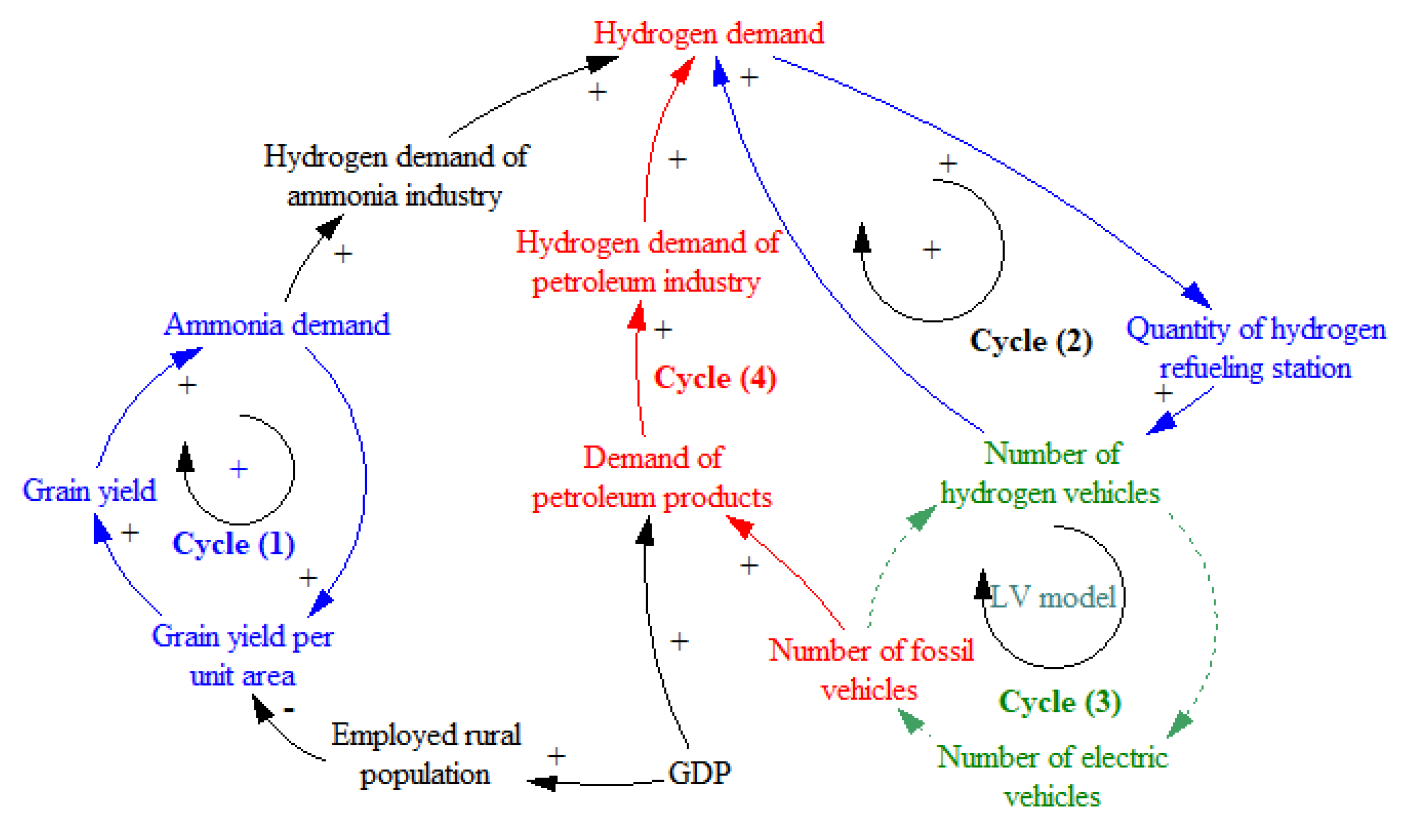
3.1. Structural Analysis of a Hydrogen Demand System

In this study, hydrogen demand mainly comes from the synthetic ammonia industry, the petroleum industry, and the hydrogen vehicle transportation industry. In addition, the development of the sectors is impacted by the macro-environment. The influence relationship and dynamic cycle process between specific factors in GDP, population, industrial development, and the corresponding hydrogen demand are shown in Figure 2. In causality, positive feedback (“+”) is defined as a facilitation relationship between factors; negative feedback (“−”) is defined as an inhibition relationship between elements; and the vehicle system, which is a feedback loop with unknown relationship, is determined through the LV model.
In Figure 2, four causality cycles are included:
  • Grain yield per unit area → grain yield → synthetic ammonia demand. The grain yield per unit area and synthetic ammonia demand cycle is a positive feedback loop. However, since GDP → employed rural population → grain yield per unit area is a negative feedback loop, with the increase in GDP, the hydrogen demand of the ammonia industry should be inhibited.
  • Hydrogen vehicle volume → hydrogen demand → quantity of hydrogen refueling stations. The hydrogen vehicle volume–quantity of hydrogen refueling station cycles is a positive feedback loop.
  • Hydrogen vehicle volume → electric vehicle volume → fossil fuel vehicle volume. The type of the vehicle volume’s feedback loop is unknown. An increase in hydrogen vehicles will influence the volume of fossil fuel and electric vehicles and then further affect the demand for hydrogen and petroleum fuels. The inner relationship could be one of competition, substitution, or promotion. To determine the relationship, the LV theory was adopted.
  • Fossil vehicle volume → demand of petroleum products → hydrogen demand of petroleum refining → hydrogen demand. The fossil vehicle volume–hydrogen demand cycle is affected by the vehicle volume feedback loop, and the relationship is determined by the result of the LV model.
As for the four causality cycles, cycle (1) is a relatively independent positive feedback subsystem. Cycle (2) and cycle (4) are influenced by cycle (3). The hydrogen demand between causality cycles represented in Figure 2 is interactive. Specifically, the factor of GDP as an exogenous variable of the hydrogen demand system impacts the hydrogen demand from both the petroleum refining cycle and the vehicle cycle. On the one hand, the production of diesel and gasoline from the petroleum refining industry will affect the fuel supply of fossil fuel vehicles in the vehicle market and then affect the competitiveness of traditional energy vehicles; on the other hand, the competitive volume of traditional, electric, and hydrogen energy vehicles in the vehicle market will also affect the production of the petroleum refining industry. To sum up, the operation of the economy–industry–hydrogen demand is a dynamic cycle process. Therefore, an SD model is constructed in this paper.
The SD model is mainly composed of three subsystems: the synthetic ammonia subsystem, the petroleum refining subsystem, and the vehicle subsystem. This paper will explain the operation mechanism and specific formula of the SD model from the above three subsystems. The following assumptions exist in the construction process of the SD model:
Hypothesis 1.
There is no speculation in the market, and all market participants are rational economic men.
Hypothesis 2.
The scope of the study is limited to the three hydrogen demand industries, namely the synthetic ammonia industry, the petroleum refining industry, and the vehicle market, regardless of cross-border transactions of hydrogen demand industries.
Before the introduction of the detailed formulation, we first list the symbols and their explanations in Table 3.

3.2. Synthetic Ammonia Subsystem

Since synthetic ammonia is mainly used for nitrogen fertilizer production and chemical products in China [4], we simplify the demand of synthetic ammonia into agricultural synthetic ammonia demand and synthetic ammonia for industrial use. To simplify the model, we assumed the proportion of agricultural use and industrial use to be 80% and 20%, respectively, according to the statistical data in [4]. The simplified model structure is shown in Figure 3.
The hydrogen demand of the synthetic ammonia industry in the t-th year is as follows:
H s , t = ( Q a s , t + Q i s , t ) × α s
where H s , t represents the hydrogen demand of synthetic ammonia production. Q a s , t and Q i s , t are the demand of synthetic ammonia for agricultural use and for industrial use. α s is the unit hydrogen consumption of synthetic ammonia production. The demand for synthetic ammonia for agricultural use consists of the grain yield and the policy of zero-growth of chemical fertilizers [37]. The zero-growth of chemical fertilizers aims to reduce the growth rate of chemical fertilizer use and strive to achieve zero growth of chemical fertilizer use by 2020. To reveal the quantitative relationship between the variables of Q a s , t , Q g , t , and the influence of zero-growth of chemical fertilizer policy, based on the empirical data of the years 2003–2019 from the national bureau of statistics of China and using regressive analysis, the equation is presented as follows:
Q a s , t = π Q 1 + π Q 2 · Q g , t + π Q 3 · γ c f
where π Q 1 , π Q 2 , and π Q 3 are regression coefficients. We define γ c f as an auxiliary binary variable. When the zero-growth policy is implemented, γ c f is 1; otherwise, γ c f is 0. Annual grain yield is determined by cultivated area and grain yield per unit area. Through regressive analysis, cultivated area is influenced by the time series factor and the red line of farmland policy [38]. The policy emphasizes the importance of ensuring the national farmland area and defines a red line of 1.8 billion mu.
Q g , t = A t × q g , t
A t = π A 1 + π A 2 · A t 1 + π A 3 · γ r l
π A 1 , π A 2 , and π A 3 are regression coefficients. γ r l is an auxiliary binary variable; when γ r l = 1 , the red line of farmland policy is implemented, otherwise γ r l = 0 .
q g , t = π q 1 + π q 2 · N p , t + π q 3 · e π q 4 · Q a s , t 1
where the grain yield per unit area is influenced by the employed rural population and the nitrogen fertilizer demand of the t 1 year. π q 1 , π q 2 , π q 3 , and π q 4 are regressive coefficients. The relationship between employed rural population and GDP is described by the Cobb–Douglas production function, and according to [39], the function is as follows:
G D P t = 1.948 10 8 K t 0.355 N p , t 3.756 A t 0.022
K t and A t represent the input of capital and the impact of technology development.
Using the ordinary least squares (OLS) method, the regression models of Equations (2), (4) and (5) were fitted to the year data from 2003 to 2017. The estimated parameters are shown in Table 4. The comparison between the simulated data and real data and the calculation results of hydrogen demand in the synthetic ammonia subsystem are presented in Section 4.

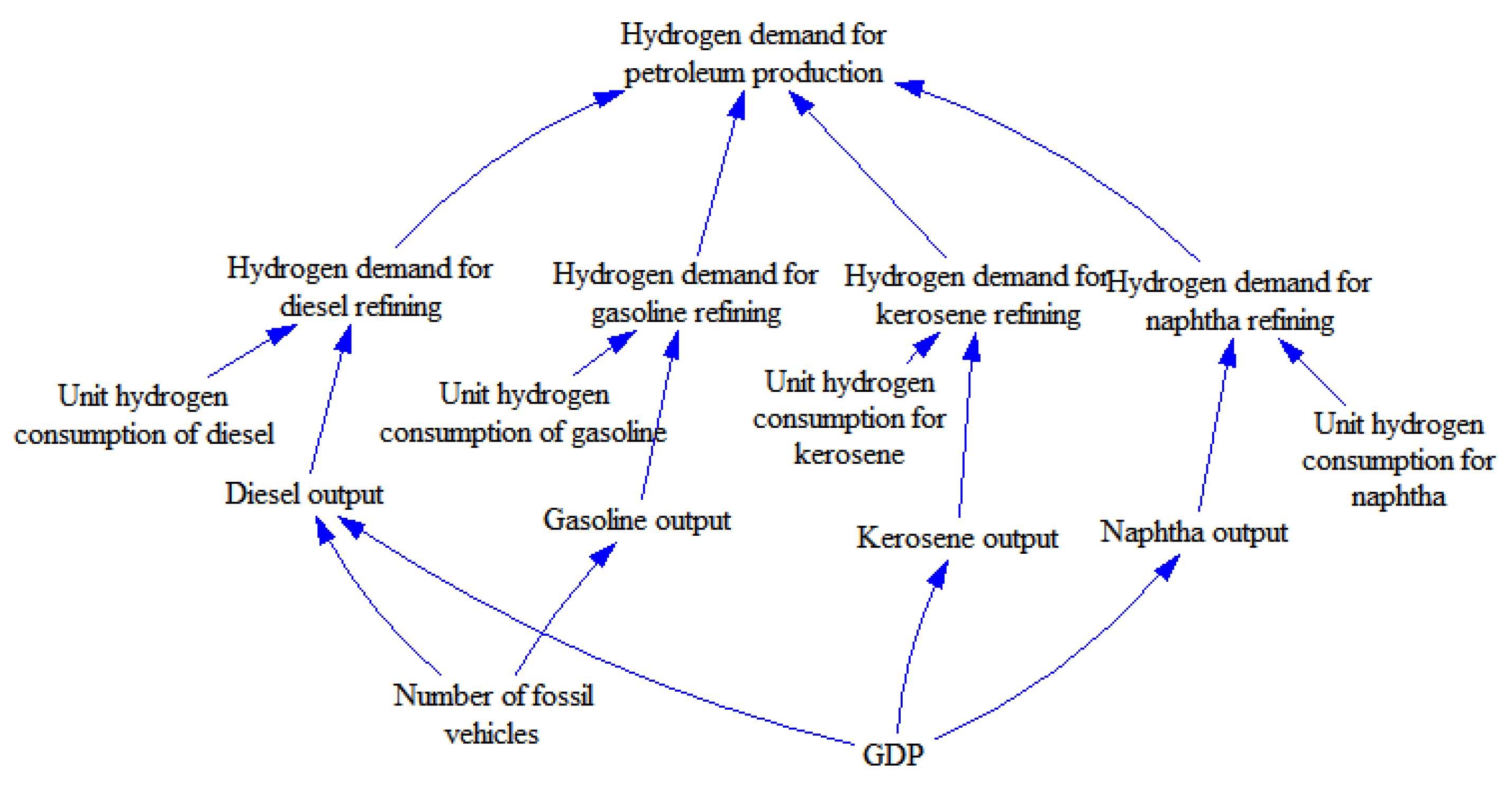
3.3. Petroleum Refining Subsystem

In the petroleum refining industry, hydrogen is mainly used for naphtha hydrodesulfurization and diesel hydrodesulfurization. Hydrogen is also used for kerosene hydrodesulfurization and hydrocracking of gasoline production. Hydrocracking is a catalytic process in the presence of hydrogen. In the petroleum refining industry, hydrogen consumption is determined by raw materials and processing technology [4]. According to the production proportion of petroleum refining products of Sinopec (China’s largest supplier of refined oil and petrochemical products and the world’s largest oil refining company), gasoline accounts for 31%, diesel accounts for 48%, kerosene accounts for 10%, naphtha accounts for 10%, and the rest are other products. The model structure of the petroleum industry subsystem refers to the major product composition of Sinopec as shown in Figure 4. The hydrogen demand for petroleum production in the t-th year is affected by the hydrogen demand of diesel refining, gasoline refining, kerosene refining, and naphtha refining as follows:
H p , t = H d r , t + H g r , t + H k r , t + H n r , t
H d r , t = Q d r , t × α d r
H g r , t = Q g r , t × α g r
H k r , t = Q k r , t × α k r
H n r , t = Q n r , t × α n r
where the hydrogen demand for diesel refining in the t-th year is made up of the output of diesel in the year t and the unit hydrogen consumption. Additionally, the hydrogen demands of gasoline refining, kerosene refining, and naphtha refining in year t are made up of the output of gasoline, kerosene, naphtha, and the unit hydrogen consumption, correspondingly. There is a power function relation between the output of diesel and the number of fossil vehicles, and a linear relation with GDP. The equation is as follows:
Q d r , t = π d r 1 + π d r 2 · π d r 3 · N v , t π d r 4 + π d r 5 · G D P t
where π d r 1 , π d r 2 , π d r 3 , π d r 4 , and π d r 5 are regression coefficients. The relationship between the output of gasoline and the number of fossil vehicles is represented as follows:
Q g r , t = π g r 1 · N v , t π g r 2
where π g r 1 and π g r 2 are regression coefficients. There is a linear relationship between the output of kerosene and GDP, and the output of naphtha is also linear with GDP. The equations are as following:
Q k r , t = π k r 1 + π k r 2 · G D P t
Q n r , t = π n r 1 + π n r 2 · G D P t
where π k r 1 and π k r 2 are the regression coefficients of Equation (14), and π n r 1 and π n r 2 are the regression coefficients of Equation (15).
Using ordinary least squares (OLS), the regression models of Equations (12)–(15) were fitted to the year data from 2003 to 2017. The estimated parameters are shown in Table 5. To calculate the hydrogen demand for petroleum production, the unit hydrogen consumption of diesel, gasoline, kerosene, and naphtha was taken from [4], and the values of the parameters and the calculation results are shown in Section 4.

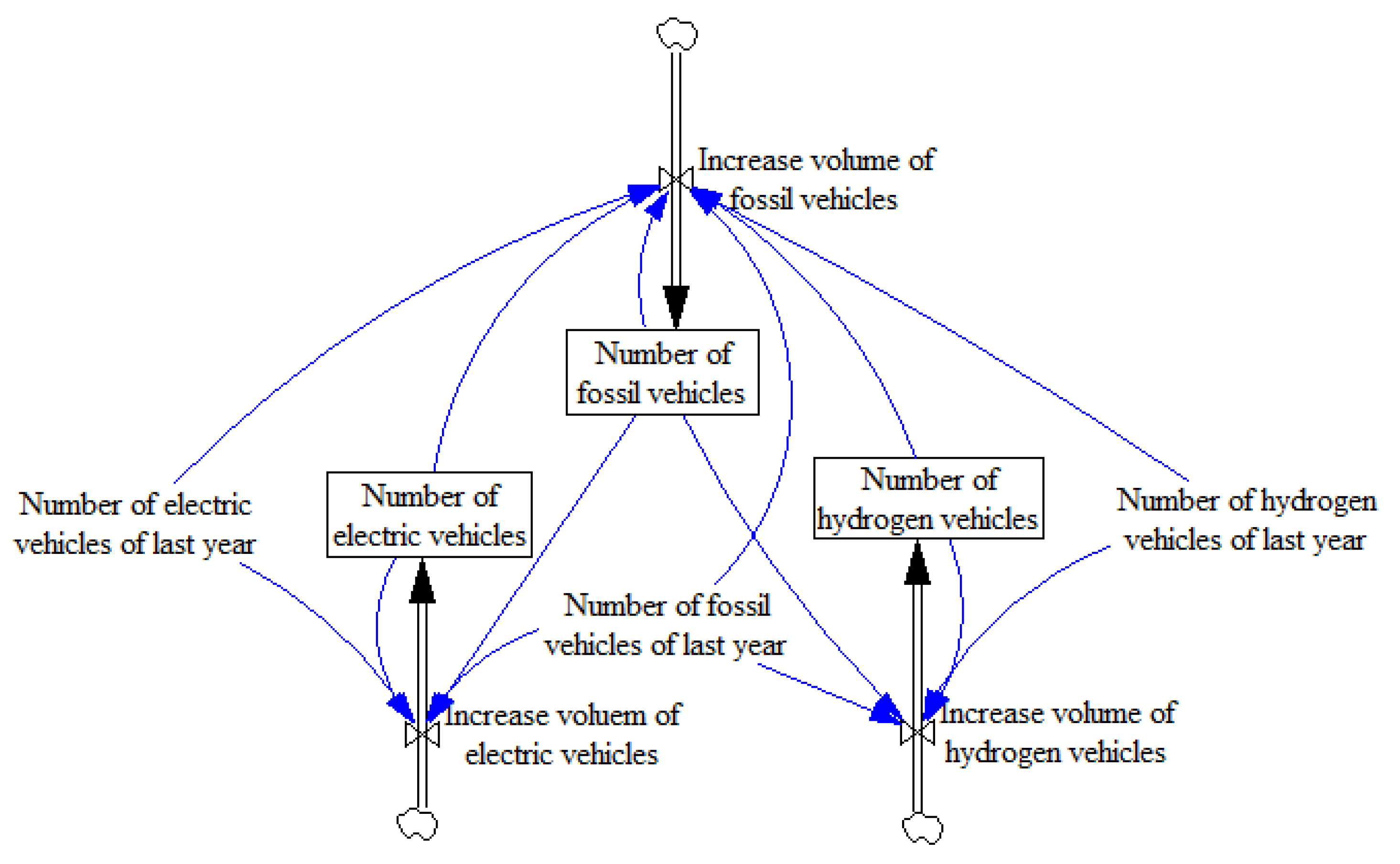
3.4. Vehicle Subsystem

For the vehicle subsystem, the architecture of the LV model is illustrated in Figure 5. In the LV model, fossil fuel vehicles play as prey, and electric and hydrogen vehicles play as predators in the vehicle market.
The predator–prey interaction consists of a pair of first-order autonomous ordinary differential equations as follows. The evolution of the number of preys is modeled by:
N ˙ v , t = N v , t ( γ v α 1 N h , t α 2 N e , t )
where N ˙ v , t = d N v , t / d t . The amount of prey, N v , t , increases with its own growth rate γ v , and decreases with the attacks of predators, which are hydrogen vehicles and electric vehicles. This decrease depends on the amount of predators N h , t , N e , t , the attack rate α 1 , α 2 of the predators, and the amount of available preys. The unit of the rate of attack is time 1 predator 1 . The number of predators evolves similarly:
N ˙ h , t = N h , t ( ϵ 1 N v , t γ h )
N ˙ e , t = N e , t ( ϵ 2 N v , t γ e )
where N ˙ h , t = d N h , t / d t , N ˙ e , t = d N e , t / d t . Prey is replaced by predators in the system with efficiencies ϵ 1 and ϵ 2 , correspondingly. The unit of the efficiency is time 1 prey 1 . It simply means that the growth rate is mostly driven by the available food supply (the preys). However, predators compete for the supply; a negative sign is associated with the growth rates γ h and γ e , correspondingly.
For the traditional predator–prey LV model above, the growth rate was modeled as linear. This means the vehicles are expected to grow without a cap. However, in reality, the growth is expected to eventually decline due to several factors: (i) the availability of fuel; (ii) the maturity of the technology; (iii) the introduction of more desirable and sustainable alternatives [18]. Considering the supply of fuel, without the relationship description with other vehicles in the market (refer to the reduction of Maryam [18]), Equation (16) is modified to:
N ˙ v , t = m i ˙ m i N v , t + m ˙ m i = γ v N v , t + μ v
where m is the total mass of fuel used by the fossil vehicles, per year, m ˙ = d m / d t . m i is the fuel used by per fossil vehicle, m i ˙ = d m i / d t , and
m = N v , t × m i
and we note γ v = m i ˙ m i and μ v = m ˙ m i . The quantity γ v is the mass of fuel used annually by a car divided by the mass of fuel consumed by a car, which corresponds to a growth rate, and it can be approximated by a constant without a breakthrough in technology. The quantity μ v is the mass of fuel used annually divided by the mass of fuel consumed by a car. Then, we combined Equation (19) with Equations (16)–(18), and the modified LV models are represented as follows:
N ˙ v , t = N v , t ( γ v α 1 N h , t α 2 N e , t ) + μ v N ˙ h , t = N h , t ( ϵ 1 N v , t γ h ) + μ h N ˙ e , t = N e , t ( ϵ 2 N v , t γ e ) + μ e
where μ v , μ h , and μ e represent the maximum number of new vehicles that can be sustained, on a yearly basis, by the supply chain of fuel. The attack rates α 1 , α 2 and efficiency rates ϵ 1 , ϵ 2 rates translate how the policies influence the number of vehicles. Since the development of hydrogen vehicles is still in its initial stage, the current market share of hydrogen vehicles is very limited. Under the current vehicle market share without considering the hydrogen vehicles, the LV model of Equation (21) is transformed to:
N ˙ v , t = N v , t ( γ v α 2 N e , t ) + μ v N ˙ e , t = N e , t ( ϵ 2 N v , t γ e ) + μ e
To estimate the unknown parameters of the modified LV model, a GM(1,1) model of the grey forecasting method was constructed. The GM(1,1) model is the most common grey prediction model, which has been successfully applied for LV model estimation [34,40]. The grey method has gained an important role in making accurate predictions for uncertain systems with small samples and incomplete information [41,42]. The main purpose of the theory is to predict the behavior of systems that cannot be detected with stochastic or fuzzy methods with limited data [43]. Therefore, with limited sample data regarding hydrogen and electric vehicles, in order to analyze the predator–prey behavior that is revealed by the LV model, the grey method was adopted.
GM(1,1) is based on the following essential steps [44]:
(1)
Accumulated generating operation (AGO): First, discretize the time series data achieved from Equation (21) as follows:
N i ˙ = ( N ˙ i , 1 , N ˙ i , 2 , . . . , N ˙ i , n ) , { t = 1 , 2 , . . . n , n 4 }
where N i is an N ˙ i one-order accumulated generating operation (AGO) sequence, that is,
N i = t = 1 n N ˙ i , t , { t = 1 , 2 , . . . n , n 4 }
(2)
Grey modeling: Form GM(1,1) model by establishing a first-order grey differential equation:
N ˙ i , t + a Z i , t = b
where
Z i , t = ( N i , t + N i , t 1 ) / 2
In Equation (25), a is called the development coefficient and b is called the driving coefficient. Combining with the GM(1,1) model, the discrete equations of (21) are transferred as follows:
N v , t N v , t 1 = γ v N v , t + N v , t 1 2 α 1 ( N v , t + N v , t 1 2 ) ( N h , t + N h , t 1 2 ) α 2 ( N v , t + N v , t 1 2 ) ( N e , t + N e , t 1 2 ) + μ v
N h , t N h , t 1 = γ h N h , t + N h , t 1 2 + ϵ 1 ( N v , t + N v , t 1 2 ) ( N h , t + N h , t 1 2 ) + μ h
N e , t N e , t 1 = γ e N e , t + N e , t 1 2 + ϵ 2 ( N v , t + N v , t 1 2 ) ( N e , t + N e , t 1 2 ) + μ e
Applying the least squares method, the coefficients can be estimated as:
A i = a b = B i T B i 1 B i T Y i , n
where
Y v , n = ( N v , 2 N v , 1 ) ( N v , t N v , t 1 ) T ,
A v = γ v α 1 α 2 μ v T ,
Y h , n = ( N h , 2 N h , 1 ) ( N h , t N h , t 1 ) T ,
A h = γ h ϵ 1 μ h T ,
Y e , n = ( N e , 2 N e , 1 ) ( N e , t N e , t 1 ) T ,
A e = γ e ϵ 2 μ e T
Hence, the AGO grey prediction model can be obtained. The growth rate parameters γ v , γ h , and γ e are related to the settling time. It describes the dynamics of the organic growth of the vehicles driven by the available resources. The efficiency and attack rates ϵ 1 , ϵ 2 , α 1 , and α 2 are mathematically related to the interactions between the vehicles. Practically, it translates the incentive of switching from a type of vehicle to another type of vehicle. According to the value rage of the efficiency ( α 1 and α 2 ) and attack rates ( ϵ 1 and ϵ 2 ), four situations are summarized. We take α 1 and ϵ 1 as an example.
(1)
When α 1 > 0 , ϵ 1 > 0 , fossil fuel vehicles and hydrogen vehicles are in the stage of mutual competition;
(2)
When α 1 > 0 , ϵ 1 < 0 , hydrogen vehicles are replacing fossil fuel vehicles;
(3)
When α 1 > 0 , ϵ 1 < 0 , fossil fuel vehicles are replacing hydrogen vehicles;
(4)
When α 1 < 0 , ϵ 1 < 0 , fossil fuel vehicles and hydrogen vehicles are promoting the development of each other.

4. Analysis

4.1. Data

To ensure the accuracy and authenticity of the model simulation and enable it to better simulate China’s hydrogen demand from the synthetic ammonia industry, petroleum industry, and the vehicle industry, in this paper we set the training data sample of the synthetic ammonia subsystem and petroleum subsystem of the model as 2003–2017, the training data sample of the vehicle subsystem as 2010–2017, and the running step length as one year. The mean absolute percentage error (MAPE) and the root mean square error (RMSE) are used to test the forecast accuracy between a data point Y i and a point produced by the model E ( Y i ) since they are considered as the best-known predictive accuracy indices for non-seasonal time series [45].
M A P E = i = 1 N N Y i E ( Y i ) Y i ; R M S E = i = 1 N ( Y i E ( Y i ) ) 2 N
Data resources of exogenous variables and the training data of endogenous variables are listed in Table 6. The setting of parameters is as follows: For synthetic ammonia production, according to [29], 0.331 mg of hydrogen is consumed for every 1.875 mg of produced ammonia. The values of the parameters of unit hydrogen consumption in the petroleum subsystem are α d r = 73.8 (kg hydrogen per ton diesel), α g r = 26.7 (kg hydrogen per ton gasoline), α k r = 7.12 (kg hydrogen per ton kerosene), and α n r = 49.84 (kg hydrogen per ton naphtha). According to the trial operation data of hydrogen energy passenger cars in Sichuan Province, the average hydrogen consumption per 100 kilometers is 3.4 kg. Assuming that the annual operating kilometers of hydrogen energy buses are 41,000 (data source: China urban passenger transport development report), each hydrogen energy bus’s average yearly hydrogen consumption is 1.394 tons.

4.2. Scenarios

Because the development of the hydrogen industry is still in its initial stage and the application of hydrogen vehicles is limited, there are not enough sample data of the number of hydrogen vehicles at present. To examine the future influence of hydrogen vehicles on the system, three scenarios are defined considering the influence of policy implementation and technology development as follows:
(1)
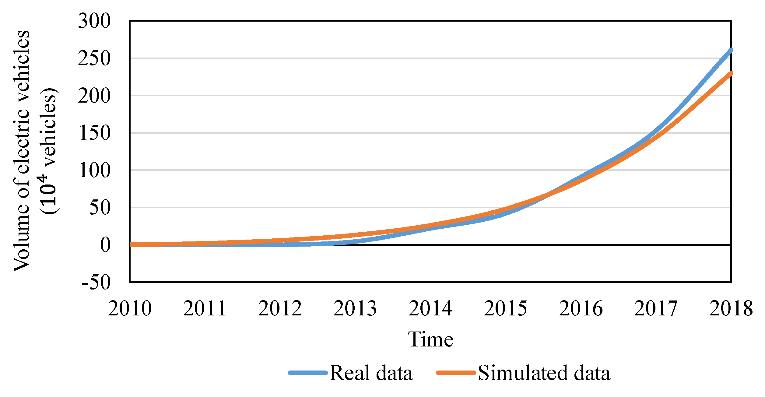
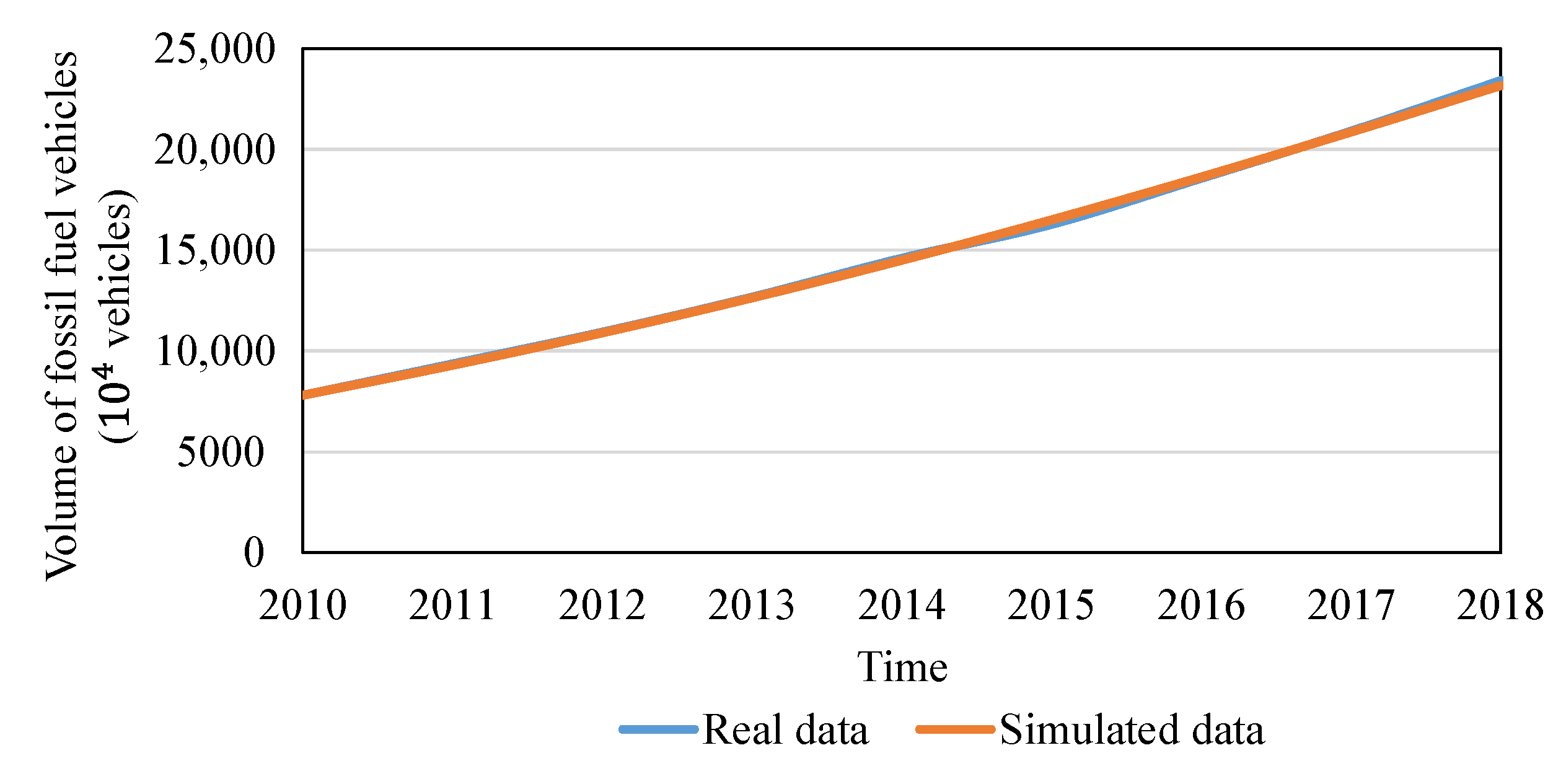
Benchmark scenario: Without considering the hydrogen vehicles, the simplified LV model refers to Equation (22). To estimate the values of the parameters, we use the historical data of the number of fossil fuel vehicles and the number of electric vehicles from the years 2010 to 2017. The values of parameters are estimated as γ v = 0.0795 , α 2 = 0.0001 , μ v = 840.8 of fossil vehicles and γ e = 1.006 , ϵ 2 = 0.000023 , μ e = 1.613 of electric vehicles.
(2)
Competition scenario: Hydrogen vehicles enter market competition, while other internal and external factors remain unchanged. Under the competition scenario, we set γ h = 0.5 , ϵ 1 = 0.00002 , μ h = 0.3 , and α 1 = 0.00001 .
(3)
Fossil fuel vehicles exit scenario: Fossil vehicles generally exit the market, policy support benefits the development of electric vehicles and hydrogen vehicles, and other internal and external factors remain unchanged. Under the fossil fuel vehicles exit scenario, we set γ h = 1 , γ v = 0.01 , ϵ 1 = 0.00004 , and μ h = 0.3 .

4.3. Results and Discussions

4.3.1. Analysis of Vehicle Subsystem

Under the benchmark scenario, without considering the influence of hydrogen vehicles, α 2 > 0 and ϵ 2 < 0 , which means that under the benchmark scenario, the electric vehicles replace fossil fuel vehicles. The comparison between the real data and simulated data from years 2010 to 2018 of the benchmark scenario is shown in Figure 6 and Figure 7. The MAPE and RMSE of electric vehicles are 9.03% and 14.38, respectively; the MAPE and RMSE of fossil fuel vehicles are 0.15% and 224.75, respectively. The results indicate that the developed simulation model captures the growth of the vehicles.
The volumes of vehicles under different scenarios are shown in Figure 8, Figure 9 and Figure 10. In Figure 8, the base year is 2010, and the end year is 2030. In Figure 9 and Figure 10, the base year is 2018, and the end year is 2030.
According to the results under the three scenarios, we found:
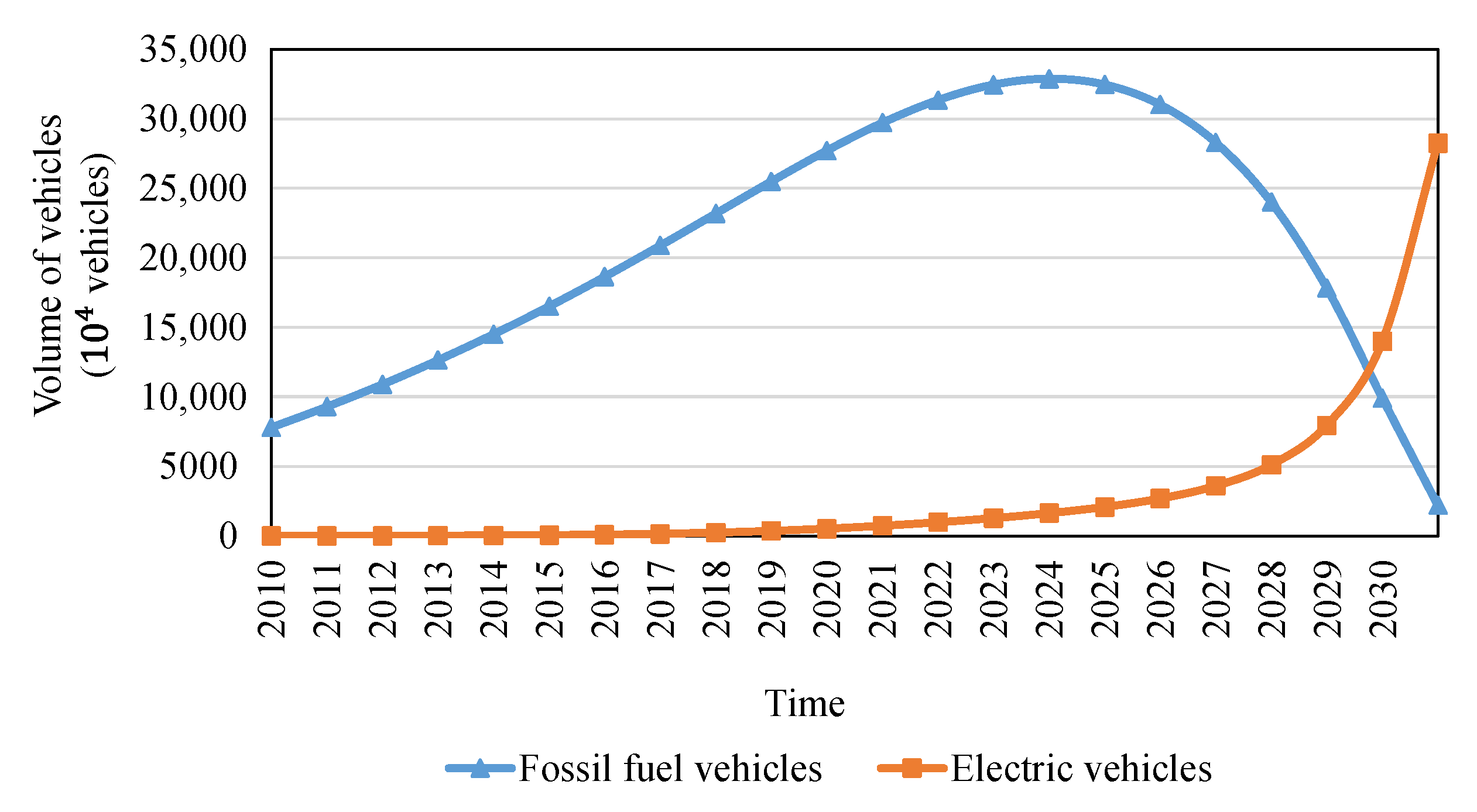
  • Under the benchmark scenario, the number of fossil fuel vehicles will reach a peak of nearly 350 million in the year 2025. With a quick flow of fossil fuel vehicles after 2025, electric vehicles will rapidly rise around 2028. The intersection point of fossil fuel vehicles and electric vehicles will arrive in 2030. At that time, the amount of fossil fuel and electric vehicles will be 99.03 million and 139.79 million, respectively.
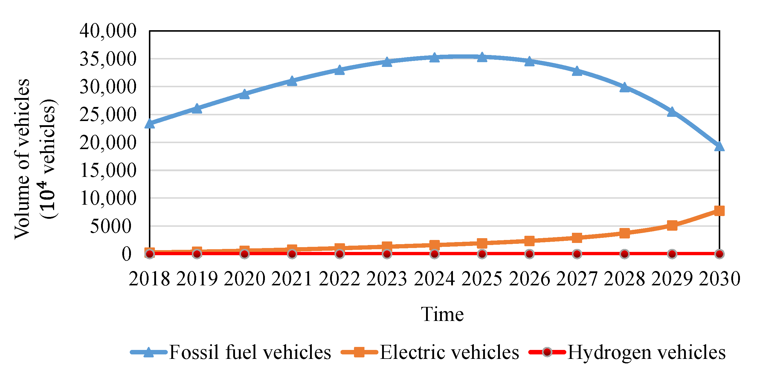
  • Under the competition scenario, the number of fossil fuel vehicles will also reach a peak of 350 million around 2025. However, compared with the benchmark scenario, the increase and decrease in fossil fuel vehicles have slowed. The entrance of hydrogen vehicles reduces the growth of electric vehicles. By the year 2030, the number of fossil fuel, electric, and hydrogen vehicles will be 193.35 million, 77.64 million, and 0.03 million, respectively.
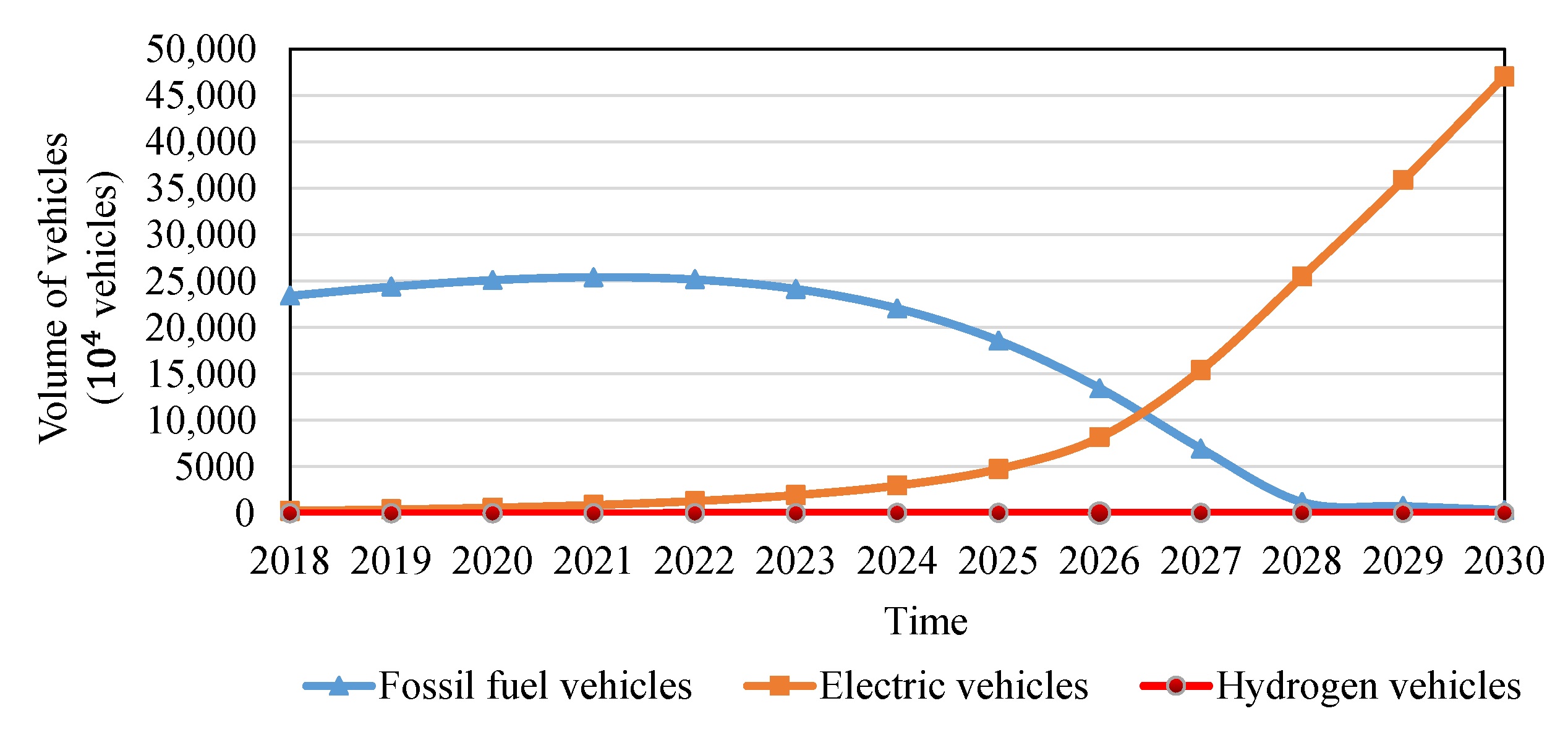
  • Under the fossil fuel vehicle exit scenario, the peak time of fossil fuel vehicles is advanced to the year 2022 as 251.65 million, and the intersection point of fossil fuel vehicles and electric vehicles is advanced to the year 2026. The automotive market will be dominated by electric vehicles. Compared to the competition scenario, the number of hydrogen vehicles has increased. By the year 2030, the amount of fossil fuel, electric, and hydrogen vehicles will be 3.12 million, 470.25 million, and 0.34 million, respectively.
  • In general, under the current hydrogen technical and infrastructure level, the scale of hydrogen vehicles will still be limited in 2030. The scale of fossil fuel vehicles will grow smaller after 2025, and electric vehicles will gradually monopolize the market.

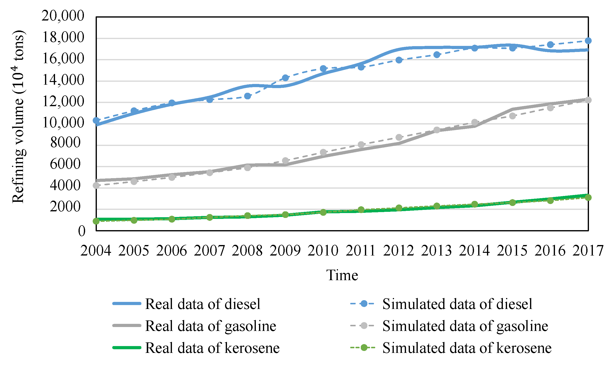
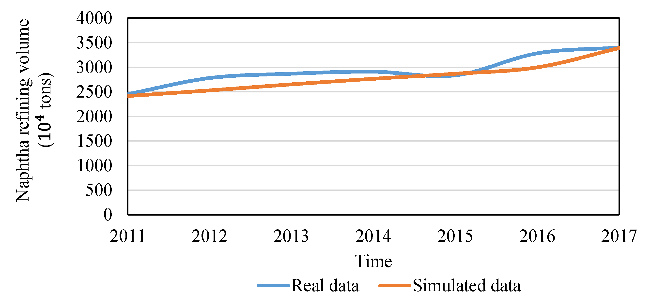
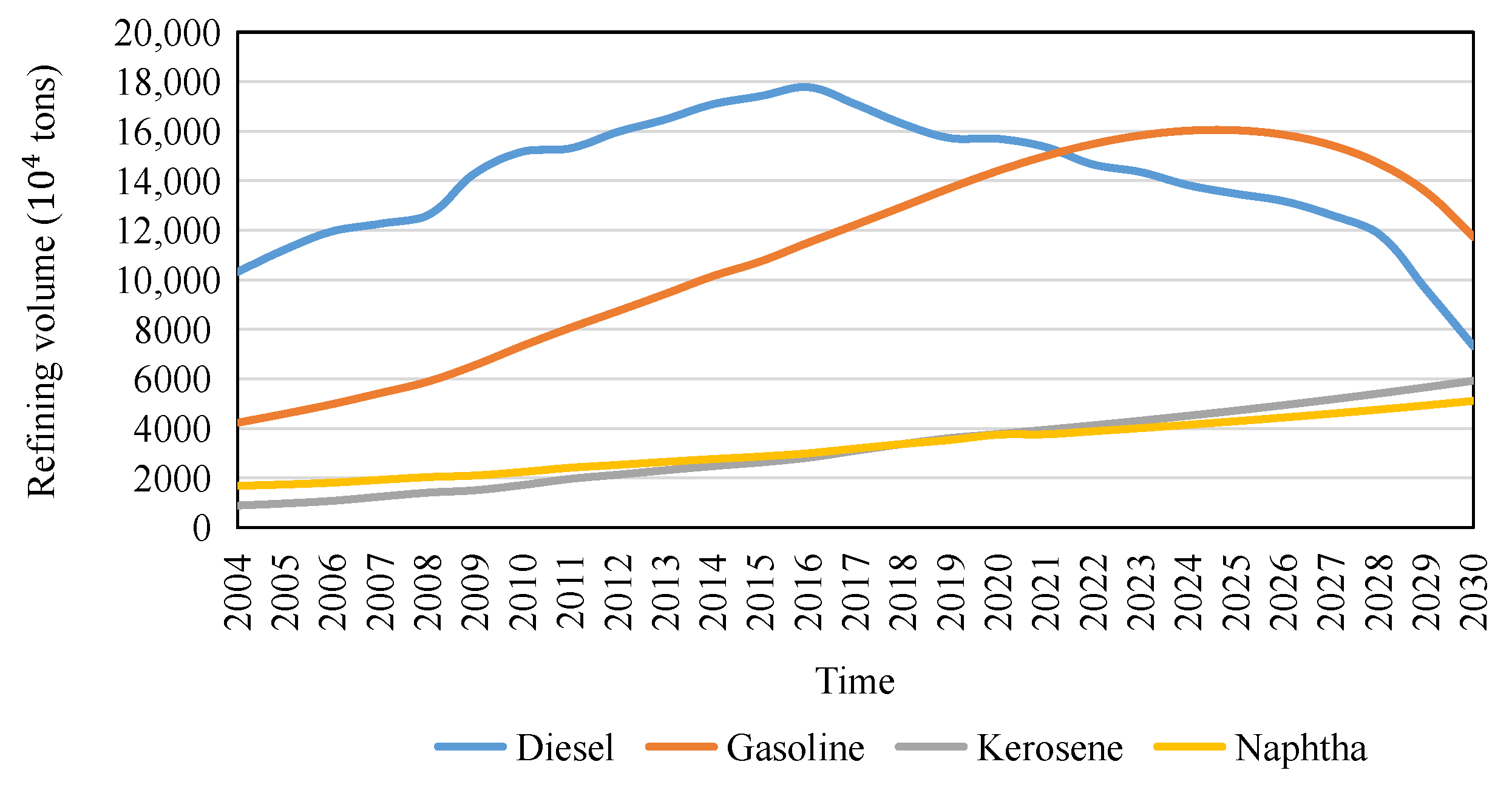
4.3.2. Analysis of Petroleum Refining Subsystem

To verify the simulation model of the petroleum industry subsystem, we compared the empirical data and simulated data of the diesel refining volume, gasoline refining volume, and kerosene refining volume from the years 2004 to 2017 in Figure 11. Due to limited statistical data, the data of naphtha refining volume used in Figure 12 are from the years 2011 to 2017. The MAPE values of diesel refining volume, gasoline refining volume, kerosene refining volume, and naphtha refining volume are 3.4%, 4.62%, 6.36%, and 5.3%, respectively, and the RMSE values are 578.19, 372.46, 128.78, and 257.93, respectively, because the evolution of fossil fuel vehicles directly influences the fuel demand of diesel and gasoline. Combing the output results of the competitive scenario of the vehicle subsystem, the simulated refining volume of the petroleum industry from 2004 to 2030 is shown in Figure 13.
The simulated results reveal that the production volume of diesel is locating in a downward path since the year 2016, and the decline will accelerate from the year 2028; the production volume of gasoline will reach the peak value around the year 2025; the kerosene and naphtha production volumes will keep rising with the increase in GDP.

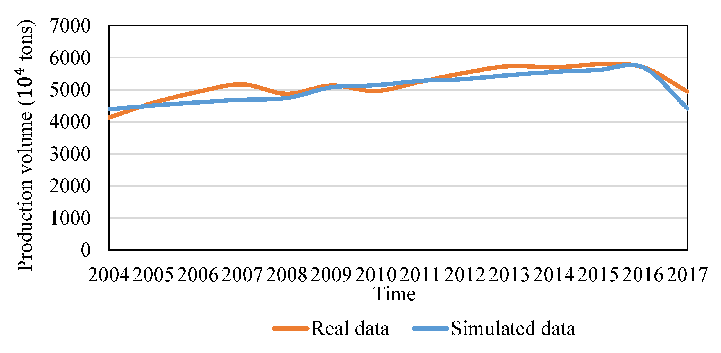
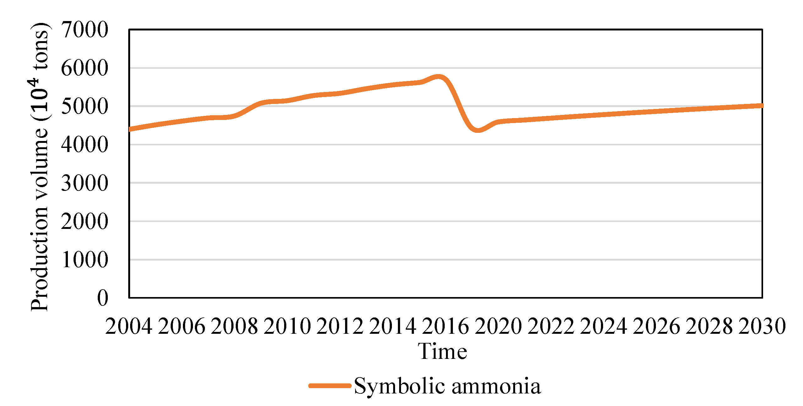
4.3.3. Analysis of Synthetic Ammonia Subsystem

To verify the simulation model of the synthetic ammonia industry subsystem, we compared the empirical data and simulated data of synthetic ammonia production volume from the years 2004 to 2017, as shown in Figure 14. The MAPE is 3.96%, and the RMSE is 245.01. The simulated synthetic ammonia production from 2004 to 2030 is shown in Figure 15.
The production volume of synthetic ammonia shows an inflection point in the year 2016. A possible reason is that the zero-growth of the chemical fertilizer policy has affected the usage of ammonia fertilizers. Although the zero-growth policy has reduced the demand for ammonia fertilizers, the red-line of farmland area policy has led to a necessary fertilizer demand. There will be a slow rise in the production volume of synthetic ammonia in the next ten years.

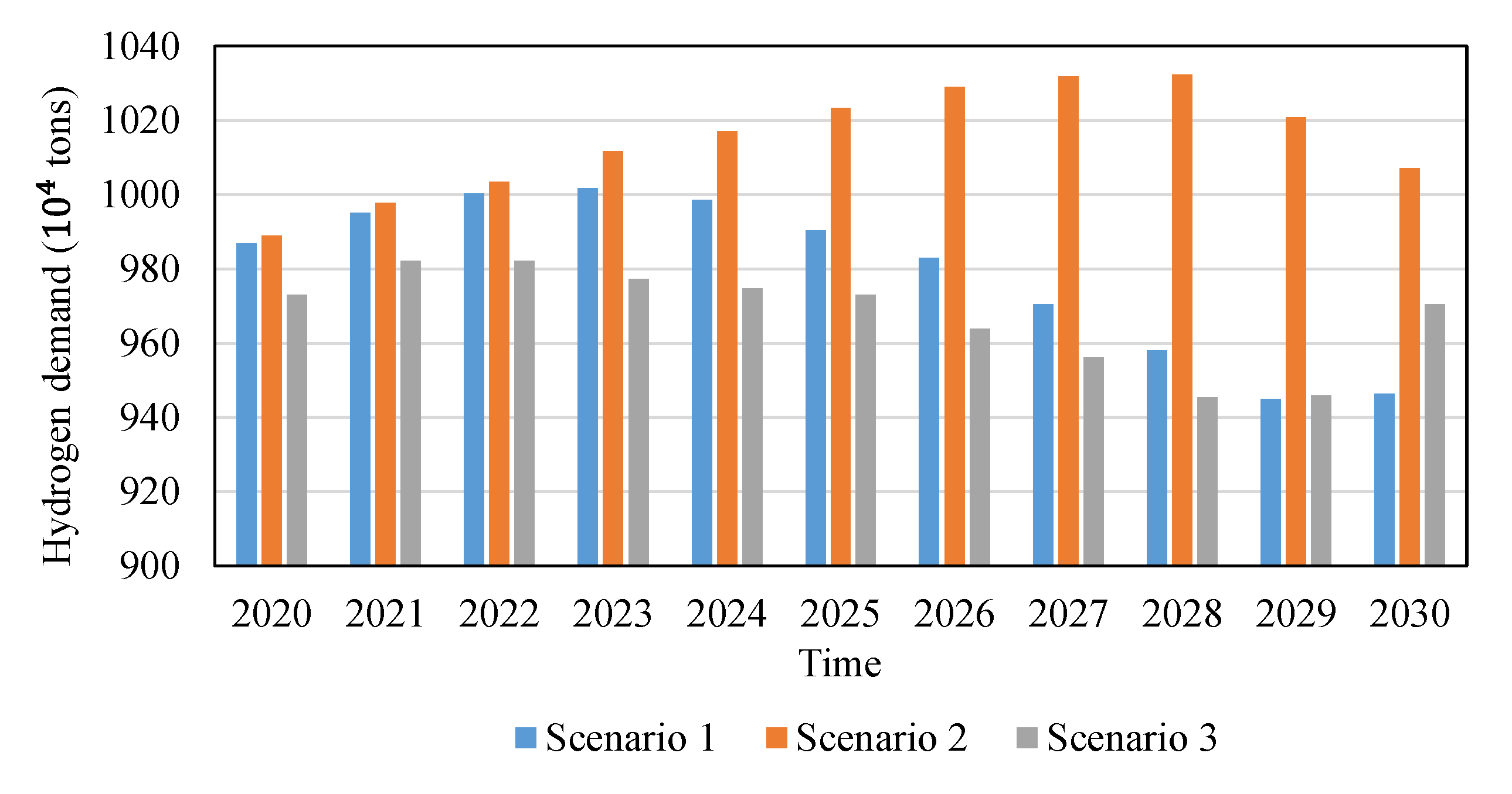
4.3.4. Analysis of Hydrogen Demand

Based on the simulated production volume of synthetic ammonia and petroleum products, and considering the development of vehicle transportation simulated in the vehicle subsystem under the three scenarios, we can estimate the hydrogen demand by 2030. The hydrogen demand in the next ten years is presented in Figure 16. Under scenario (1), the maximum hydrogen demand volume appears in 2023 as 10.01 million tons and then generally reduces to 9.46 million tons. Under scenario (2), the maximum volume of hydrogen demand appears in 2028 as 10.32 million tons and then reduces to 10.07 million tons by the year 2030. Under scenario (3), the maximum hydrogen demand volume appears in 2022 as 9.82 million tons and then reduces. However, the inflection point from decrease to increase occurs in 2028, and the minimum volume is 9.45 million tons. By the year 2030, the volume comes to 9.7 million tons. Under scenario (3), hydrogen demand will increase by the year 2029. As the reduction of the number of traditional vehicles will increase in the next decade, the development momentum of hydrogen vehicles will gradually rise after the year 2029.
  • The decrease in fossil fuel vehicles will lead to a reduction in hydrogen demand. Although the development of hydrogen vehicles will promote the increase in hydrogen demand, the high cost, immature technology, and inadequate charging facilities of hydrogen vehicles have restrained the rapid growth of hydrogen vehicles. Without substantial policy support, the demand for hydrogen from hydrogen energy vehicles will remain limited in the next ten years. If policymakers accelerate the withdrawal of fossil energy vehicles from the market, the demand for hydrogen is expected to usher in an upward path around 2029.
  • Although the change of hydrogen demand in the petroleum refining and vehicle industries has a specific impact on the total hydrogen demand, the minimum hydrogen demand can be guaranteed at 9.4 million tons, a difference of 870,000 tons from the maximum need. This is because the hydrogen demand for the production of synthetic ammonia accounts for a large proportion. Affected by the rigid demand for agricultural production, the demand for ammonia fertilizer will hardly decline on a large scale.

5. Conclusions

This paper proposed a nationwide hydrogen demand simulation model combining system dynamics and the Lotka–Volterra approach. In the model, the hydrogen demand from traditional hydrogen consumption industries of synthetic ammonia and petroleum refining and the newly developing hydrogen vehicle market were discussed. The exogenous variables of population, macro-economy, and the impact of support policies were considered to analyze the evolution of hydrogen demand. In addition, to verify the impact from supporting policies, the scenarios of hydrogen vehicles entering market competition and fossil fuel vehicles exiting the market are analyzed compared with the current benchmark scenario. The simulation results demonstrate the effectiveness of the proposed model and provide some useful forward-looking guidance for the policy makers.
  • China’s population and agricultural production scale determine the rigid demand for ammonia fertilizer products. The hydrogen demand in ammonia fertilizer production will reach 8.8 million tons by 2030.
  • Policy orientation plays a vital role in promoting the development of hydrogen energy in the petroleum refining and vehicle market. However, it will still be challenging for hydrogen energy to become the mainstream energy by 2030 because of the competition from electric vehicles, even if traditional energy vehicles gradually withdraw from the market. The obstacles come from the supply capacity and production cost of green hydrogen, the development level of hydrogen fuel cell technology, and the construction level of facilities.
In future research, to forecast the hydrogen demand more comprehensively, more hydrogen consumption industries need to be considered in the model, such as methanol production and steel smelting, etc. In addition, the evolution of the fully competitive vehicle market is affected by complex internal and external factors. This paper has made some hypotheses and simplifications, and more influencing factors and variable relationships should be expanded upon.

Author Contributions

Conceptualization, J.H. and W.L.; methodology, J.H. and W.L.; writing—original draft preparation, J.H.; supervision and funding support, W.L.; writing—review and editing, X.W. All authors have read and agreed to the published version of the manuscript.

Funding

This paper has been supported by Construction Project of Baoding Low Carbon Economy Industry Research Institute (1106/9100615009).

Institutional Review Board Statement

Not applicable.

Informed Consent Statement

Not applicable.

Data Availability Statement

Not applicable.

Conflicts of Interest

The authors declare no conflict of interest.

References

  1. Abad, A.V.; Dodds, P.E. Green hydrogen characterisation initiatives: Definitions, standards, guarantees of origin, and challenges. Energy Policy 2020, 138, 111300. [Google Scholar] [CrossRef]
  2. Ball, M.; Wietschel, M. The future of hydrogen—Opportunities and challenges. Int. J. Hydrogen Energy 2009, 34, 615–627. [Google Scholar] [CrossRef]
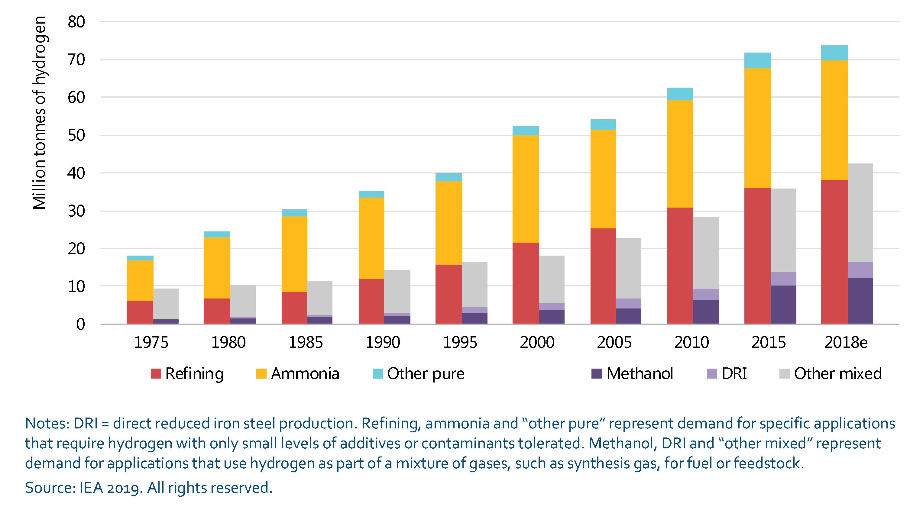
  3. International Energy Agency. The Future of Hydrogen: Seizing Today’s Opportunities. Available online: www.iea.org/reports/the-future-of-hydrogen (accessed on 10 June 2019).
  4. Bai, X. An analysis on the production and consumption of hydrogen in the world and China. Chem. Ind. 2003, 21, 18–25. [Google Scholar]
  5. Mohammadi, A.; Mehrpooya, M. A comprehensive review on coupling different types of electrolyzer to renewable energy sources. Energy 2018, 158, 632–655. [Google Scholar] [CrossRef]
  6. Moon, J.-i. Remarks by President Moon Jae-In at Presentation for Hydrogen Economy Roadmap and Ulsan’s Future Energy Strategy; Office of the President: Seoul, Korea, 2019.
  7. METI. Formulation of a New Strategic Roadmap for Hydrogen and Fuel Cells; Agency for Natural Resources and Energy, Ed.; Ministry of Economy: Tokyo, Japan, 2019.
  8. ARENA. Hydrogen Offers Significant Exporting Potential for Australia; Australian Renewable Energy Agency: Canberra, Australia, 2018.
  9. Quarton, C.J.; Samsatli, S. How to incentivise hydrogen energy technologies for net zero: Whole-system value chain optimisation of policy scenarios. Sustain. Prod. Consum. 2021, 27, 1215–1238. [Google Scholar] [CrossRef]
  10. General Office of the State Council. Available online: http://www.gov.cn/zhengce/content/2020-11/02/content_5556716.htm (accessed on 2 November 2020).
  11. Information Office of Shandong Provincial People’s Government. Available online: http://www.scio.gov.cn/m/xwfbh/gssxwfbh/xwfbh/shandong/Document/1682774/1682774.htm (accessed on 4 June 2020).
  12. NEA of Inner Mongolia. Available online: http://nyj.nmg.gov.cn/tzgg/gg/202107/t20210715_1788442.html (accessed on 15 July 2021).
  13. The People’s Government of Sichuan Province. 2020. Available online: http://http://www.sc.gov.cn/10462/10464/10465/10574/2020/9/22/8ef70cb7baf441db8cd2a9b754bed940.shtml (accessed on 22 September 2020).
  14. Ma, T.; Sun, B.; Guo, H.; Ji, J.; Jiang, M. Evaluation on hydrogen consumption and its reduction of CO2 emission of Chinese medium and long-term economic development. Int. J. Hydrogen Energy 2017, 42, 19376–19388. [Google Scholar]
  15. Wang, G. Advanced vehicles: Costs, energy use, and macroeconomic impacts. J. Power Sources 2011, 196, 530–540. [Google Scholar] [CrossRef]
  16. Sang, Y.P.; Kim, J.W.; Lee, D.H. Development of a market penetration forecasting model for Hydrogen Fuel Cell Vehicles considering infrastructure and cost reduction effects. Energy Policy 2011, 39, 3307–3315. [Google Scholar]
  17. Shafiei, E.; Davidsdottir, B.; Leaver, J.; Stefansson, H.; Asgeirsson, E.I. Energy, economic, and mitigation cost implications of transition toward a carbon-neutral transport sector: A simulation-based comparison between hydrogen and electricity. J. Clean. Prod. 2017, 141, 237–247. [Google Scholar] [CrossRef]
  18. Sahdia, M.; Florimond, G. Forecasting the Evolution of Hydrogen Vehicle Fleet in the UK using Growth and Lotka-Volterra Models. arXiv 2021, arXiv:2102.04771. [Google Scholar]
  19. Hong, T.; Pinson, P.; Wang, Y.; Weron, R.; Yang, D.; Zareipour, H. Energy Forecasting: A Review and Outlook. IEEE Open Access J. Power Energy 2020, 7, 376–388. [Google Scholar] [CrossRef]
  20. Hong, T. Energy forecasting: Past, present, and future. Foresight Int. J. Appl. Forecast. 2014, 32, 43–48. [Google Scholar]
  21. Shi, H.; Xu, M.; Li, R. Deep Learning for Household Load Forecasting—A Novel Pooling Deep RNN. IEEE Trans. Smart Grid 2018, 9, 5271–5280. [Google Scholar] [CrossRef]
  22. Feng, C.; Sun, M.; Zhang, J. Reinforced Deterministic and Probabilistic Load Forecasting via Q-Learning Dynamic Model Selection. IEEE Trans. Smart Grid 2020, 11, 1377–1386. [Google Scholar] [CrossRef]
  23. Cai, L.; Gu, J.; Jin, Z. Two-Layer Transfer-Learning-Based Architecture for Short-Term Load Forecasting. IEEE Trans. Ind. Inform. 2020, 16, 1722–1732. [Google Scholar] [CrossRef]
  24. Xie, J.; Hong, T.; Stroud, J. Long-Term Retail Energy Forecasting With Consideration of Residential Customer Attrition. IEEE Trans. Smart Grid 2015, 6, 2245–2252. [Google Scholar] [CrossRef]
  25. Rafique, M.M.; Shakir, M.A.; Zahid, I.; Chohan, G.Y. An Integrated Long Term Energy Forecasting Approach for Sustainable Energy Mix in Pakistan. In Proceedings of the 2018 International Conference on Power Generation Systems and Renewable Energy Technologies (PGSRET), Islamabad, Pakistan, 10–12 September 2018; pp. 1–5. [Google Scholar]
  26. Quarton, C.J.; Tlili, O.; Welder, L.; Mansilla, C.; Blanco, H.; Heinrichs, H.; Leaver, J.; Samsatli, N.J.; Lucchese, P.; Robinius, M.; et al. The curious case of the conflicting roles of hydrogen in global energy scenarios. Sustain. Energy Fuels 2020, 4, 80–95. [Google Scholar] [CrossRef] [Green Version]
  27. Ying, Z.; Xin-gang, Z.; Zhen, W. Demand side incentive under renewable portfolio standards: A system dynamics analysis. Energy Policy 2020, 144, 111652. [Google Scholar] [CrossRef]
  28. Wu, D.; Ning, S. Dynamic assessment of urban economy-environment-energy system using system dynamics model: A case study in Beijing. Environ. Res. 2018, 164, 70–84. [Google Scholar] [CrossRef]
  29. Bicer, Y.; Dincer, I. Assessment of a Sustainable Electrochemical Ammonia Production System Using Photoelectrochemically Produced Hydrogen under Concentrated Sunlight. ACS Sustain. Chem. Eng. 2017, 5, 8035–8043. [Google Scholar] [CrossRef]
  30. Li, Z.Y.; Huang, G.S.; Ren, W.P.; Wang, H.Q. The structure adjustment and development of China’s oil refining and petrochemical industry during the 13th Five-Year Plan period. Int. Pet. Econ. 2016, 24, 88–96. [Google Scholar]
  31. Li, Y.; Kimura, S. Economic competitiveness and environmental implications of hydrogen energy and fuel cell electric vehicles in ASEAN countries: The current and future scenarios. Energy Policy 2021, 148, 111980. [Google Scholar] [CrossRef]
  32. Zheng, W.; Jitsuro, S. A necessary and sufficient condition for global asymptotic stability of time-varying Lotka-Volterra predator-prey systems. Nonlinear Anal. Theory Methods Appl. 2015, 127, 128–142. [Google Scholar] [CrossRef]
  33. Hung, H.C.; Tsai, Y.S.; Wu, M.C. A Modified Lotka-Volterra Model for Competition Forecasting in Taiwan’s Retail Industry. Comput. Ind. Eng. 2014, 77, 70–79. [Google Scholar] [CrossRef]
  34. Tsai, B.H.; Chang, C.J.; Chang, C.H. Elucidating the Consumption and CO2 Emissions of Fossil Fuels and Low-carbon Energy in the United States Using Lotka-Volterra Models. Energy 2016, 100, 416–424. [Google Scholar] [CrossRef]
  35. Ziegler, A.M.; Brunner, N.; Kühleitner, M. The Markets of Green Cars of Three Countries: Analysis Using Lotka-Volterra and Bertalanffy-Pütter Models. J. Open Innov. Technol. Mark. Complex 2020, 6, 67. [Google Scholar] [CrossRef]
  36. Wang, Y.; Xu, T.; Pang, T.Z. The Study of Feedback Relationship with SD Model Based on LV: Application in Transportation System. J. Wuhan Univ. Technol. (Transp. Sci. Eng.) 2020. Available online: https://kns.cnki.net/kcms/detail/42.1824.U.20201009.1428.014.html (accessed on 15 December 2021).
  37. Ministry of Agriculture and Rural Affairs of the People’s Republic of China. 2017. Available online: http://www.moa.gov.cn/nybgb/2015/san/201711/t20171129_5923401.htm (accessed on 29 November 2017).
  38. The Central People’s Government of the People’s Republic of China. 2008. Available online: http://www.gov.cn/govweb/jrzg/2008-11/23/content_1156819.htm (accessed on 23 November 2008).
  39. Li, X. Empirical analysis of Cobb Douglas production function of China’s economic growth. Peoples Tribune 2015, 12, 89–91. [Google Scholar]
  40. Lee, S.; Lee, D.; Oh, H. Technological Forecasting at the Korean Stock Market: A Dynamic Competition Analysis Using Lotka-Volterra Model. Technol. Forecast. Soc. Chang. 2005, 72, 1044–1057. [Google Scholar] [CrossRef]
  41. Deng, J.-L. Control problem of grey systemes. Syst. Control Lett. 1982, 1, 288–294. [Google Scholar]
  42. Lin, Y.; Liu, S. A historical introduction to grey systems theory. In Proceedings of the IEEE International Conference on System, Man and Cybernetics, The Hague, The Netherlands, 10–13 October 2004; pp. 2403–2408. [Google Scholar]
  43. Liu, S.; Lin, Y. Grey Information: Theory and Practical Applications; Springer: Berlin/Heidelberg, Germany, 2006. [Google Scholar]
  44. Hamzacebi, C.; Es, H.A. Forecasting the annual electricity consumption of Turkey using an optimized grey model. Energy 2014, 70, 165–171. [Google Scholar] [CrossRef]
  45. Hyndman, R.J.; Koehler, A.B. Another look at measures of forecast accuracy. Int. J. Forecast. 2006, 22, 679–688. [Google Scholar] [CrossRef] [Green Version]
Figure 1. Global hydrogen demand from 1975 to 2018.
Mathematics 10 00205 g001
Figure 2. Interaction between macro-economy, industry development, and hydrogen demand.
Mathematics 10 00205 g002
Figure 3. Model of synthetic ammonia subsystem.
Mathematics 10 00205 g003
Figure 4. Model of petroleum refining subsystem.
Mathematics 10 00205 g004
Figure 5. The architecture of the LV model.
Mathematics 10 00205 g005
Figure 6. Compare the number of electric vehicles with real data and simulated data.
Mathematics 10 00205 g006
Figure 7. Compare the number of fossil fuel vehicles with real data and simulated data.
Mathematics 10 00205 g007
Figure 8. Number of fossil fuel vehicles and electric vehicles under the benchmark scenario.
Mathematics 10 00205 g008
Figure 9. Number of vehicles under the competition scenario.
Mathematics 10 00205 g009
Figure 10. Number of vehicles under the fossil fuel vehicles exit scenario.
Mathematics 10 00205 g010
Figure 11. Compare the volume of diesel refining, gasoline refining, and kerosene refining with real data and simulated data.
Mathematics 10 00205 g011
Figure 12. Compare the volume of naphtha refining with real data and simulated data.
Mathematics 10 00205 g012
Figure 13. Refining volume of petroleum industry simulated until the year 2030.
Mathematics 10 00205 g013
Figure 14. Comparison of the production volume of synthetic ammonia with real data and simulated data.
Mathematics 10 00205 g014
Figure 15. Synthetic ammonia production volume simulated until the year 2030.
Mathematics 10 00205 g015
Figure 16. Hydrogen demand simulated until the year 2030.
Mathematics 10 00205 g016
Table 1. Selected hydrogen-related government policies announced in China since 2020.
AreaAnnouncements and Incentive Policies Since Year 2020
ChinaThe General Office of the State Council issued the New Energy
Vehicle Industry Development Plan (2021–2035) to promote the
development of facilities and technologies of hydrogen energy
storage and transportation, hydrogenation stations, and on-board
hydrogen storage [10].
ShandongPublished the Development Plan of Hydrogen Industry (2020–2030)
to develop the production of green hydrogen, hydrogen storage, and
hydrogenation stations. Targets are set to the year 2030 [11].
Inner MongoliaFor 2024–2025, the production capacity of green hydrogen will reach
500,000 tons/year; cultivate and introduce 15–20 core enterprises
related to hydrogen energy; build 100 hydrogen refueling stations;
and promote more than 10,000 fuel cell vehicles [12].
SichuanProposition to build Sichuan into a domestic and international well-
known hydrogen energy industry base; demonstrate application
on characteristic area and green hydrogen output bases [13].
Table 2. Major differences between representative references and this paper.
No.Prediction SubjectTimeMethodologyImpact Factors
[14]HydrogenLong-termSDMacroeconomic growth rate
development trend of first,
second, and third industries
[15]VehiclesLong-termCGE modelMacroeconomic impacts,
policy incentives, and
technology development
[16,17]VehiclesLong-termSDMacroeconomic impacts,
policy incentives, technology
development, and electricity
transition pathways
[18]VehiclesLong-termLVPolicy incentives, fuel supply,
technology development
[21,22,23]LoadShort-termAI/MLHistorical load
[24]Retail energyLong-termRegression,
survival analysis
Customer attrition and
load per customer
[25]Load and
energy
Long-termLEAPMacroeconomic impacts,
energy policies, energy supply
This
paper
HydrogenLong-termSD, LV,
scenario analysis
Macroeconomic growth rate,
population, policy incentives,
development of hydrogen
consumption industries, and
hydrogen fuel cell technology
Table 3. Variables and explanations.
VariablesUnitExplanation
Synthetic ammonia subsystem
H t m 3 Hydrogen demand of the t-th year
H s , t m 3 Hydrogen demand of synthetic ammonia
production in year t
Q a s , t tonDemand of synthetic ammonia for agricultural
use in year t
Q i s , t tonDemand of synthetic ammonia in year t
for industrial use
α s m 3 /tonUnit hydrogen consumption of synthetic
ammonia production
Q g , t tonGrain annual yield of the t-th year
γ c f -Auxiliary binary variable of zero-growth
of chemical fertilizer policy
A t muCultivated area in year t
q g , t ton/muGrain yield per unit area
γ r l -Auxiliary binary variable of the red line
policy of farmland area policy
N p , t 10 millionEmployed rural population in year t
Petroleum refining subsystem
H p , t m 3 Hydrogen demand for petroleum production
in the t-th year
H d r , t m 3 Hydrogen demand for diesel refining in year t
H g r , t m 3 Hydrogen demand for gasoline refining in year t
H k r , t m 3 Hydrogen demand for kerosene refining in year t
H n r , t m 3 Hydrogen demand for naphtha refining in year t
Q d r , t 10 4 tonDiesel output in year t
Q g r , t 10 4 tonGasoline output in year t
Q k r , t 10 4 tonKerosene output in year t
Q n r , t tonNaphtha output in year t
α d r m 3 /tonUnit hydrogen consumption of diesel refining
α g r m 3 /tonUnit hydrogen consumption of gasoline refining
α k r m 3 /tonUnit hydrogen consumption of kerosene refining
α n r m 3 /tonUnit hydrogen consumption of naphtha refining
G D P t -Gross domestic product in year t
Vehicle subsystem
N v , t 10 4 The number of fossil vehicles in year t
N h , t 10 4 The number of hydrogen vehicles in year t
N e , t 10 4 The number of electric vehicles in year t
γ v -The growth rate of fossil vehicles
γ h -The growth rate of hydrogen vehicles
γ e -The growth rate of electric vehicles
μ v -The available resource for fossil vehicles
μ h -The available resource for hydrogen vehicles
μ e -The available resource for electric vehicles
α 1 -The attack rate of hydrogen vehicles
α 2 -The attack rate of electric vehicles
ϵ 1 -The efficiency rate of hydrogen vehicles
ϵ 2 -The efficiency rate of electric vehicles
Table 4. The estimated parameters of the synthetic ammonia subsystem.
VariablesCoefficient EstimatesStandard Deviationp-Value
Equation (2)
Q a s , t 0.053.6940.003
γ c f −1059.5−4.0870.001
Constant π Q 1 12341.4850.06
Coefficient of determination: 0.55, F-test p-value: 0.003
Adjusted coefficient of determination: 0.62
Equation (4)
A t 1 −0.36880.320.003
γ r l 2.35410.680.002
Constant π A 1 25.528.680.08
Coefficient of determination: 0.60, F-test p-value: 0.002
Adjusted coefficient of determination: 0.66
Equation (5)
N p , t −0.056−5.790.0001
Q a s , t 1 0.000130.000040.0001
e 0.00013 Q a s , t 1 42.510.250.09
Constant π q 1 4353.84.720.0008
Coefficient of determination: 0.83, F-test p-value: 4.69 × 10 5
Adjusted coefficient of determination: 0.86
Table 5. The estimated parameters of the petroleum refining subsystem.
VariablesCoefficient
Estimates
Standard Deviationp-Value
Equation (12)
N f , t 0.24480.024 2.86 × 10 7
N f , t 0.2448 160435.410.0007
1604 × N f , t 0.2448 3.8810.9380.0016
G D P t −0.03170.010.01
Constant π d r 1 −27,59089.870.01
Coefficient of determination: 0.949, F-test p-value: 7.77 × 10 8
Adjusted coefficient of determination: 0.939
Equation (13)
N f , t 0.51780.02 5.16 × 10 11
Constant π g r 1 70.7815.810.0008
Coefficient of determination: 0.940, F-test p-value: 3.52 × 10 6
Adjusted coefficient of determination: 0.941
Equation (14)
G D P t 0.0033 1.7 × 10 4 2.94 × 10 10
Constant π k r 1 353.68.920.0018
Coefficient of determination: 0.967, F-test p-value: 2.94 × 10 10
Adjusted coefficient of determination: 0.964
Equation (15)
G D P t 0.0025 4.2 × 10 4 0.002
Constant π n r 1 131727.90.005
Coefficient of determination: 0.87, F-test p-value: 0.002
Adjusted coefficient of determination: 0.85
Table 6. Data resources of exogenous and endogenous variables.
Exogenous VariableData Resource
GDPNational Bureau of Statistics
Employed rural populationNational Bureau of Statistics
Zero-growth of chemical
fertilizer policy
China’s Department of Agriculture
Red line policy of farmland
area
China’s Ministry of Land and
Resources
Endogenous VariableData Resource
Cultivated areaChina’s Ministry of Land and
Resources
Grain yield per unit areaNational Bureau of Statistics
Agricultural synthetic ammonia
demand
National Bureau of Statistics
Diesel output, gasoline output,
kerosene output, and naphtha output
National Bureau of Statistics
Number of fossil fuel vehiclesNational Bureau of Statistics
Number of electric vehiclesiimedia data (data.iimedia.cn, 15 December 2021)
Publisher’s Note: MDPI stays neutral with regard to jurisdictional claims in published maps and institutional affiliations.

