A Direct Prediction of the Shape Parameter in the Collocation Method of Solving Poisson Equation

Abstract

In this paper, we totally discard the traditional trial-and-error algorithms of choosing the acceptable shape parameter c in the multiquadrics $-\sqrt{c^2+{\parallel x\parallel }^2}$ when dealing with differential equations, for example, the Poisson equation, with the RBF collocation method. Instead, we choose c directly by the MN-curve theory and hence avoid the time-consuming steps of solving a linear system required by each trial of the c value in the traditional methods. The quality of the c value thus obtained is supported by the newly born choice theory of the shape parameter. Experiments demonstrate that the approximation error of the approximate solution to the differential equation is very close to the best approximation error among all possible choices of c.

1. Introduction

The generalized multiquadrics are defined as

$$\begin{array}{c}\hfill \varphi \left(x\right):={(-1)}^{\lceil \beta /2\rceil }(c^2+{\parallel x\parallel }^2{)}^{\beta /2},\beta \in R\setminus 2N_{\ge 0},c>0,x\in R^d,\end{array}$$

(1)

where $\lceil \beta /2\rceil$ denotes the smallest integer greater than or equal to $\beta /2$ and the constant c is called the shape parameter. These are the most popular radial basis functions (RBFs) and are frequently used in the collocation method of solving partial differential equations. In this paper, we let $\beta =1$. In the collocation method, an approximate solution to a differential equation is of the form

$$\begin{array}{c}\hfill \widehat{u}\left(x\right):=\sum _{i=1}^N{\lambda }_i\varphi (x-x_i)+p\left(x\right),\end{array}$$

(2)

where $p\left(x\right)\in P_{m-1}$, the space of polynomials of a degree less than or equal to $m-1$ in $R^d$, and $X=\{x_1,\dots ,x_N\}$ is a set of points scattered in the domain. For $m=0,P_{m-1}:=\left\{0\right\}$. The integer $m:=\lceil \beta /2\rceil$. Since we let $\beta =1$, here $m=1$ and $p\left(x\right)$ is a constant ${\lambda }_0$. An unorthodox way even drops ${\lambda }_0$ and lets it be 0. The constants ${\lambda }_i,i=0,\dots ,N$, are chosen so that $\widehat{u}\left(x\right)$ satisfies the differential equation (including the boundary conditions) at the points $x_i,i=1,\dots ,N$, called the collocation points.

The function $\widehat{u}\left(x\right)$ originates from the interpolation theory of the radial basis functions, where $\widehat{u}\left(x\right)$ interpolates a given function $f\left(x\right)$ at $x_1,\dots ,x_N$. It is required that ${\sum }_{i=1}^N{\lambda }_i{p}_l\left(x_i\right)=0$ for $l=1,\dots Q$, where $\{p_1,\cdots ,p_Q\}$ is a basis of $P_{m-1}$. Besides this, the only requirement for $X=\{x_1,\dots ,x_N\}$ is that it should be $P_{m-1}$-unisolvent. Namely, if $p\in P_{m-1}$ and $p\left(x_i\right)=0$ for $i=1,\dots ,N$, then $p\left(x\right)$ is a zero polynomial. Further details can be observed in Section 8.5 of Wendland [1]. This origin has to be mentioned because we need it in the design of $\widehat{u}\left(x\right)$.

This approach of solving the differential equation was first introduced by E. Kansa [2,3]. A huge amount of experiments demonstrate that it works very well. The main advantage of this approach, namely the collocation method (or Kansa method), is that the data points are scattered in the domain without meshes. Moreover, its high accuracy is also very attractive. However, the choice of the shape parameter c contained in the multiquadrics is a big problem. Experts in this field only know that it is very influential, but do not know how to choose it. G. Fasshauer [4] pointed out that only trial-and-error algorithms were available. Some people even give up using mutiquadrics to solve differential equations due to this problem. This greatly lowers the power of the collocation method. The purpose of this paper is to handle this problem.

2. Materials and Methods

2.1. Sobolev Error Estimates

We need a space that plays an intermediate role in our approximating work.

Definition 1.

For any positive number γ,

$$B_{\gamma }:=\left\{f\in L^2\left(R^d\right):\widehat{f}\left(\xi \right)=0\mathrm{if}\parallel \xi \parallel >\gamma \right\}$$

where $\widehat{f}$ denotes the Fourier transform of f. For each $f\in B_{\gamma }$, its norm is

$${\parallel f\parallel }_{B_{\gamma }}:={\left\{\int |\widehat{f}{\left(\xi \right)|}^{2}d\xi \right\}}^{1/2}.$$

Here, $f\in L^2(R^d)$ means that $f{\left(x\right)}^2$ is integrable. Our main interest is in the Sobolev space $W_2^{\tau }(R^d)$ because it contains the solutions of a lot of important differential equations. The Sobolev space is defined as follows.

Definition 2.

For any positive integer τ,

$$W_2^{\tau }(R^d)=\left\{f\in L^2(R^d):D^{k}f(x_1,\dots ,x_d)\in L^2(R^d)for|k|\le \tau \right\}$$

where $k=(k_1,\dots ,k_d)$ and $|k|={\sum }_{i=1}^d{k}_i$. The Sobolev norm is

$${\parallel f\parallel }_{W_2^{\tau }\left(R^d\right)}:={\left\{\sum _{0\le \left|k\right|\le \tau }\int {\left|D^{k}f\left(x\right)\right|}^{2}dx\right\}}^{1/2}.$$

In the preceding definition, the derivatives are more general than the classical derivatives, called the distributional derivatives. The vector k can even have negative or noninteger coordinates. Further details can be observed in Yosida [5] and any textbooks of functional analysis.

Before introducing Sobolev error estimates, some necessary ingredients should be defined. Suppose $X=\{x_1,\dots ,x_N\}\subseteq \mathsf{\Omega }$ is a finite subset of a bounded set $\mathsf{\Omega }$ in $R^d$. Then, the separation radius is defined by

$$q_X:=\frac{1}{2}\underset{i\ne j}{min}\parallel x_i-x_j\parallel .$$

Then, we have the following core theorem, which is just Theorem 3.4 of Narcowich et al. [6].

Theorem 1.

Let β, $t\in R$ satisfy $\beta >d/2$ and $t\ge 0$. If $f\in W_2^{\beta +t}(R^d)$, then there exists $f_{\gamma }\in B_{\gamma }$ such that $f_{\gamma }{{|}_X=f|}_X$ and

$$\parallel f-f_{\gamma }{\parallel }_{W_2^{\beta }(R^d)}\le 5·{\kappa }^{-t}{q}_X^t{\parallel f\parallel }_{W_2^{\beta +t}(R^d)},$$

(3)

with $\gamma =\kappa /q_X$, where $\kappa \ge 1$ depends only on β and d.

This theorem clearly shows that any function in the Sobolev space, possibly a solution to an important differential equation, can be interpolated by a $B_{\gamma }$ function with a good error bound. In the next subsection, we will demonstrate that any $B_{\gamma }$ function can be interpolated by a function of the form (2), also with a good error bound.

2.2. MN-Curve Theory

We need some basic definitions.

Definition 3.

For any positive number σ,

$$E_{\sigma }:=\left\{f\in L^2(R^d):\int {|\widehat{f}\left(\xi \right)|}^2{e}^{{|\xi |}^2/\sigma }d\xi <\infty \right\}$$

where $\widehat{f}$ denotes the Fourier transform of f. For each $f\in E_{\sigma }$, its norm is

$${\parallel f\parallel }_{E_{\sigma }}:={\left\{\int |\widehat{f}{(\xi )|}^2{e}^{{|\xi |}^2/\sigma }d\xi \right\}}^{1/2}.$$

Obviously, for any $\gamma ,\sigma >0$, $B_{\gamma }\subseteq E_{\sigma }$. We are going to demonstrate how $E_{\sigma }$ functions can be approximated by functions of the form (2).

For any set $\mathsf{\Omega }\subseteq R^d$ and any set $X=\{x_1,\dots ,x_N\}$ of sample points contained in $\mathsf{\Omega }$, the fill distance is defined by

$$\delta (\mathsf{\Omega },X):=\underset{x\in \mathsf{\Omega }}{sup}\underset{i=1,\dots ,N}{inf}\parallel x-x_i\parallel ,$$

abbreviated as $\delta$, which measures the spacing of the sample points in $\mathsf{\Omega }$. The smaller $\delta$ is, the more sample points are needed. In this paper, $\mathsf{\Omega }$ denotes the function domain.

Definition 4.

Let d and β be as in (1). The numbers ρ and ${\Delta }_0$ are defined, as follows.

(a) 

Suppose $\beta <d-3$. Let $s=\lceil (d-\beta -3)/2\rceil$. Then

(i) 

if $\beta <0,\rho =(3+s)/3and{\Delta }_0=\frac{(2+s)(1+s)\cdots 3}{{\rho }^2};$

(ii) 

if $\beta >0,\rho =1+\frac{s}{2\lceil \beta /2\rceil +3}and{\Delta }_0=\frac{(2m+2+s)(2m+1+s)\cdots (2m+3)}{{\rho }^{2m+2}}$ where $m=\lceil \beta /2\rceil$.

(b) 

Suppose $d-3\le \beta <d-1$. Then $\rho =1$ and ${\Delta }_0=1$.

(c) 

Suppose $\beta \ge d-1$. Let $s=-\lceil (d-\beta -3)/2\rceil$. Then

$$\rho =1and{\Delta }_0=\frac{1}{(2m+2)(2m+1)\cdots (2m-s+3)}wherem=⌈\beta /2⌉.$$

For any $f\in E_{\sigma }$ and $x\in \mathsf{\Omega }$, the upper bound of $|f\left(x\right)-\widehat{u}\left(x\right)|$ is a very complicated expression involving both $\rho$ and ${\Delta }_0$, as can be observed in Luh [7]. A modified theory for a purely scattered data setting can be observed in Luh [8]. In this paper, we only need to extract its essential part

$$\begin{array}{c}\hfill |f\left(x\right)-\widehat{u}{\left(x\right)|\le \mathrm{MN}\left(c\right)\parallel f\parallel }_{E_{\sigma }}\end{array}$$

(4)

where c is just the shape parameter defined in (1) and $\mathrm{MN}\left(c\right)$ is the MN function to be defined below, as in [8].

In the MN-curve theory, we require that the diameter r of the function domain $\mathsf{\Omega }$ satisfy $b_0/2\le r\le b_0$ where $b_0$ is a parameter determined by us. Once $b_0$ is fixed, there are three cases for the definition of $\mathrm{MN}\left(c\right)$.

Case 1: $\beta <0,|d+\beta |\ge 1$ and $d+\beta +1\ge 0$ Let $f\in E_{\sigma }$ and $\varphi \left(x\right)$ be as in (1). For any fixed fill distance $\delta$ satisfying $0<\delta \le b_0/2$, the optimal value of c in $[24\rho \delta ,\infty )$ is the number minimizing

$$\mathrm{MN}\left(c\right):=\left\{\begin{array}{cc}\sqrt{8\rho }{c}^{(\beta -d-1)/4}{\left\{{\left({\xi }^{\ast }\right)}^{(d+\beta +1)/2}{e}^{c{\xi }^{\ast }-{\left({\xi }^{\ast }\right)}^2/\sigma }\right\}}^{1/2}{\left(\frac{2}{3}\right)}^{c/\left(24\rho \delta \right)}\hfill & \mathrm{if} c\in [24\rho \delta ,12b_0\rho ),\hfill \\ \sqrt{\frac{2}{3b_0}}{c}^{(\beta -d+1)/4}{\left\{{\left({\xi }^{\ast }\right)}^{(d+\beta +1)/2}{e}^{c{\xi }^{\ast }-{\left({\xi }^{\ast }\right)}^2/\sigma }\right\}}^{1/2}{\left(\frac{2}{3}\right)}^{b_0/\left(2\delta \right)}\hfill & \mathrm{if} c\in [12b_0\rho ,\infty ),\hfill \end{array}\right.$$

where

$${\xi }^{\ast }=\frac{c\sigma +\sqrt{c^2{\sigma }^2+4\sigma (d+\beta +1)}}{4}.$$

Remark 1.

Note that ${lim}_{c\to 0^{+}}\mathrm{MN}\left(c\right)=\infty$ and ${lim}_{c\to \infty }\mathrm{MN}\left(c\right)=\infty$.

Case 2: $\beta =-1$ and $d=1$ Let $f\in E_{\sigma }$ and $\varphi \left(x\right)$ be as in (1). For any fill distance δ satisfying $0<\delta \le b_0/2$, the optimal value of c in $[24\rho \delta ,\infty )$ is the number minimizing

$$\mathrm{MN}\left(c\right):=\left\{\begin{array}{cc}\sqrt{8\rho }{c}^{(\beta -1)/2}{\left\{\frac{1}{ln2}+2\sqrt{3}M\left(c\right)\right\}}^{1/2}{\left(\frac{2}{3}\right)}^{c/\left(24\rho \delta \right)}\hfill & \mathit{if} c\in [24\rho \delta ,12b_0\rho ),\hfill \\ \sqrt{\frac{2}{3b_0}}{c}^{\beta /2}{\left\{\frac{1}{ln2}+2\sqrt{3}M\left(c\right)\right\}}^{1/2}{\left(\frac{2}{3}\right)}^{b_0/\left(2\delta \right)}\hfill & \mathit{if} c\in [12b_0\rho ,\infty ),\hfill \end{array}\right.$$

where

$$\mathrm{M}\left(c\right):=\left\{\begin{array}{cc}{e}^{1-1/\left(c^2\sigma \right)}\hfill & \mathit{if} 0<c\le \frac{2}{\sqrt{3\sigma }},\hfill \\ g\left(\frac{c\sigma +\sqrt{c^2{\sigma }^2+4\sigma }}{4}\right)\hfill & \mathit{if} \frac{2}{\sqrt{3\sigma }}<c,\hfill \end{array}\right.$$

g being defined by $g\left(\xi \right):=\sqrt{c\xi }{e}^{c\xi -{\xi }^2/\sigma }$.

Remark 2.

The same as Case 1, we have ${lim}_{c\to 0^{+}}\mathrm{MN}\left(c\right)=\infty$ and ${lim}_{c\to \infty }\mathrm{MN}\left(c\right)=\infty$.

Case 3: $\beta >0$ and $d\ge 1$ Let $f\in E_{\sigma }$ and $\varphi \left(x\right)$ be as in (1). For any fixed fill distance δ satisfying $0<\delta \le b_0/2$, the optimal value of c in $[24\rho \delta ,\infty )$ is the number minimizing

$$\mathrm{MN}\left(c\right):=\left\{\begin{array}{cc}\sqrt{8\rho }{c}^{(\beta -d-1)/4}{\left\{\frac{{\left({\xi }^{\ast }\right)}^{(1+\beta +d)/2}{e}^{c{\xi }^{\ast }}}{e^{{\left({\xi }^{\ast }\right)}^2/\sigma }}\right\}}^{1/2}{\left(\frac{2}{3}\right)}^{c/\left(24\rho \delta \right)}\hfill & \mathit{if} c\in [24\rho \delta ,12b_0\rho ),\hfill \\ \sqrt{\frac{2}{3b_0}}{c}^{(1+\beta -d)/4}{\left\{\frac{{\left({\xi }^{\ast }\right)}^{(1+\beta +d)/2}{e}^{c{\xi }^{\ast }}}{e^{{\left({\xi }^{\ast }\right)}^2/\sigma }}\right\}}^{1/2}{\left(\frac{2}{3}\right)}^{b_0/\left(2\delta \right)}\hfill & \mathit{if} c\in [12b_0\rho ,\infty ),\hfill \end{array}\right.$$

where

$${\xi }^{\ast }=\frac{c\sigma +\sqrt{c^2{\sigma }^2+4\sigma (1+\beta +d)}}{4}.$$

Remark 3.

(a) If $\beta -d-1>0,{lim}_{c\to 0^{+}}\mathrm{MN}\left(c\right)=0$. (b) If $\beta -d-1<0,{lim}_{c\to 0^{+}}\mathrm{MN}\left(c\right)$$=\infty$. (c) If $\beta -d-1=0,{lim}_{c\to 0^{+}}\mathrm{MN}\left(c\right)$ is a finite positive number. (d) ${lim}_{c\to \infty }\mathrm{MN}\left(c\right)=\infty$. Practically, we never let $\beta -d-1\ge 0$. Hence (a) and (c) will not happen.

In all the three cases, the requirement $c\ge 24\rho \delta$ is harmless because the value $24\rho \delta$ is usually quite small and a huge amount of experiments demonstrate that the optimal choice of c never lies in the interval $(0,24\rho \delta )$.

The function $\widehat{u}\left(x\right)$ in (4) in fact interpolates $f\left(x\right)$ at the sample points. Hence, strictly speaking, $\mathrm{MN}\left(c\right)$ can only be used to measure the quality of the function interpolation. Nevertheless, collocation is in spirit a kind of interpolation, not just approximation. We require that $\widehat{u}\left(x\right)$ satisfy the given differential equation at the sample points. Theoretically, the value c minimizing $\mathrm{MN}\left(c\right)$ should also be the optimal choice of c in the definition of $\widehat{u}\left(x\right)$ when dealing with differential equations. Another point is that in (4), it is required that $f\in E_{\sigma }$, which is mathematically just a subset of the Sobolev space $W_2^{\tau }(R^d)$. Fortunately, the Formula (3) offers a bridge for our approximating $f\in W_2^{\tau }(R^d)$ with $\widehat{u}\left(x\right)$. For a fixed set $X=\{x_1,\dots ,x_N\}$ of sample points in $\mathsf{\Omega }\subseteq R^d$, any $f\in W_2^{\tau }(R^d)$ can be interpolated by an $f_{\gamma }\in B_{\gamma }\subseteq E_{\sigma }$. Then $f_{\gamma }$ can be interpolated by $\widehat{u}$. Both happen in X. The influence of c happens in the latter part of the interpolations. Hence, we can directly predict the optimal value of c with the curve of $\mathrm{MN}\left(c\right)$. No search is needed.

2.3. Problem Setting

We try to handle Poisson equations. A standard 3D Poisson equation is of the form

$$\begin{array}{c}\hfill \left\{\begin{array}{cc}{u}_{xx}(x,y,z)+u_{yy}(x,y,z)+u_{zz}(x,y,z)=f(x,y,z)\hfill & \mathrm{for} (x,y,z)\in \mathsf{\Omega }\setminus \partial \mathsf{\Omega },\hfill \\ u(x,y,z)=g(x,y,z)\hfill & \mathrm{for} (x,y,z)\in \partial \mathsf{\Omega },\hfill \end{array}\right.\end{array}$$

(5)

where $\mathsf{\Omega }$ is the domain with boundary $\partial \mathsf{\Omega }$, and $f,g$ are given functions. A natural extension to d dimensions can be easily understood by replacing $(x,y,z)$ with $(x_1,\dots ,x_d)$ and letting $\mathsf{\Omega }\subseteq R^d$.

Our goal is to find an approximate solution $\widehat{u}\left(x\right)$ of the form (2). Our approach is to find real numbers ${\lambda }_0,\dots ,{\lambda }_N$ such that $\widehat{u}\left(x\right):={\sum }_{i=1}^N{\lambda }_i\varphi (x-x_i)+{\lambda }_0$ satisfies (5) in $R^d$ at the sample points $x_1,\dots ,x_N\in R^d$, called collocation points. The constant c appearing in $\varphi$ is determined by the MN-curve theory. Of course, this process involves solving a system of linear equations with unknowns ${\lambda }_0,\dots ,{\lambda }_N$, by requiring that

$$\begin{array}{c}\hfill \left\{\begin{array}{cc}\sum _{j=1}^N{\lambda }_j\mathcal{L}\left[\varphi (x_i-x_j)\right]=f\left(x_i\right)\hfill & \mathrm{for} i=1,\dots ,N_{int},\hfill \\ \\ \sum _{j=1}^N{\lambda }_j=0,\hfill \\ \\ \sum _{j=1}^N{\lambda }_j\varphi (x_i-x_j)+{\lambda }_0=g\left(x_i\right)\hfill & \mathrm{for} i=N_{int}+1,\dots ,N,\hfill \end{array}\right.\end{array}$$

(6)

where $\mathcal{L}$ denotes the differential operator of the Poisson equation. The sample points $x_i,\dots ,x_{N_{int}}$ are located in the interior of the domain cube, and $x_{N_{int}+1},\dots ,x_N$ on the boundary. The requirement ${\sum }_{j=1}^N{\lambda }_j=0$ results from the interpolation theory, as explained in the introduction section. We thus have an $(N+1)\times (N+1)$ system of linear equations.

Although its coefficient matrix is not sparse, it can be efficiently solved because its scale is not large, as long as the shape parameter c is well chosen. For a long time, the RBF collocation method has been severely criticized for the full matrix induced by the multiquadrics. Fortunately, now we know that the amount of sample points needed can be greatly reduced by choosing the shape parameter c according to our theory. This is exciting. As for the collocation points, they are scattered in the domain and boundary without meshes. Theoretically, if the exact solution $u\left(x\right)$ lies in the Sobolev space, the approximate solution $\widehat{u}\left(x\right)$ thus found should be quite good. Experiments demonstrate that the approximation error $|u\left(x\right)-\widehat{u}\left(x\right)|$ is indeed very small.

3. Results

The crux of this approach is the choice of the parameter $\sigma$ in the definition of $\mathrm{MN}\left(c\right)$. Once $f_{\gamma }\in B_{\gamma }$ in (3) is given, in order to measure $|f_{\gamma }\left(x\right)-\widehat{u}\left(x\right)|$, there are infinitely many possible choices of $\sigma$ for the implementation of the inequality (4). If $\sigma$ is too large, the value of $\mathrm{MN}\left(c\right)$ will be very large, making the MN curve meaningless. If $\sigma$ is very small, the value of $\mathrm{MN}\left(c\right)$ is usually very small. However, ${\parallel f\parallel }_{E_{\sigma }}$ will become extremely large, also making (4) meaningless. Fortunately, after analyzing the MN curves, we can always find a suitable $\sigma$ without much effort, as demonstrated in our experiments.

3.1. 1D Model

Although our main interest is in two and three-dimensional problems, in order to help the reader use our approach, we still include the 1D problem.

Let $u\left(x\right)=e^{-x}$ with domain $\mathsf{\Omega }=\{x:0\le x\le 1\}$ be the test function. We are going to solve

$$u_{xx}\left(x\right)=e^{-x}$$

for $0<x<1$ with $u\left(0\right)=1$ and $u\left(1\right)=e^{-1}$.

The approximate solution will be of the form $\widehat{u}\left(x\right)={\sum }_{i=1}^N\varphi (x-x_i)+{\lambda }_0$, where $\varphi \left(x\right)=-\sqrt{c^2+x^2}$ and ${\lambda }_i,i=0,\dots ,N$ are constants to be determined. The sample points $x_i,i=1,\dots ,N$, are randomly generated and scattered in the unit interval, except that two of them are 0 and 1, respectively. The choice of c will be made according to Case 3 of the MN curves.

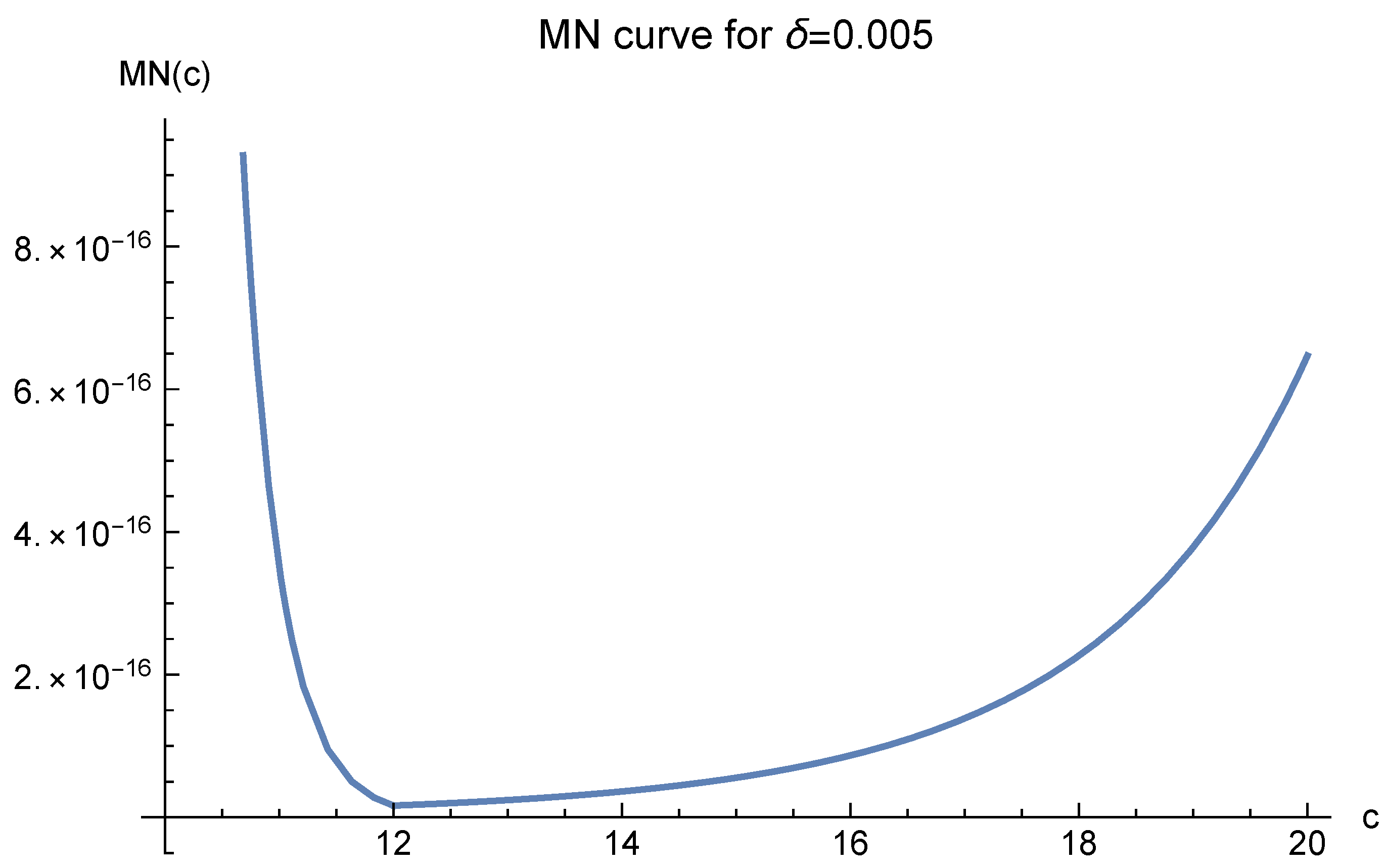
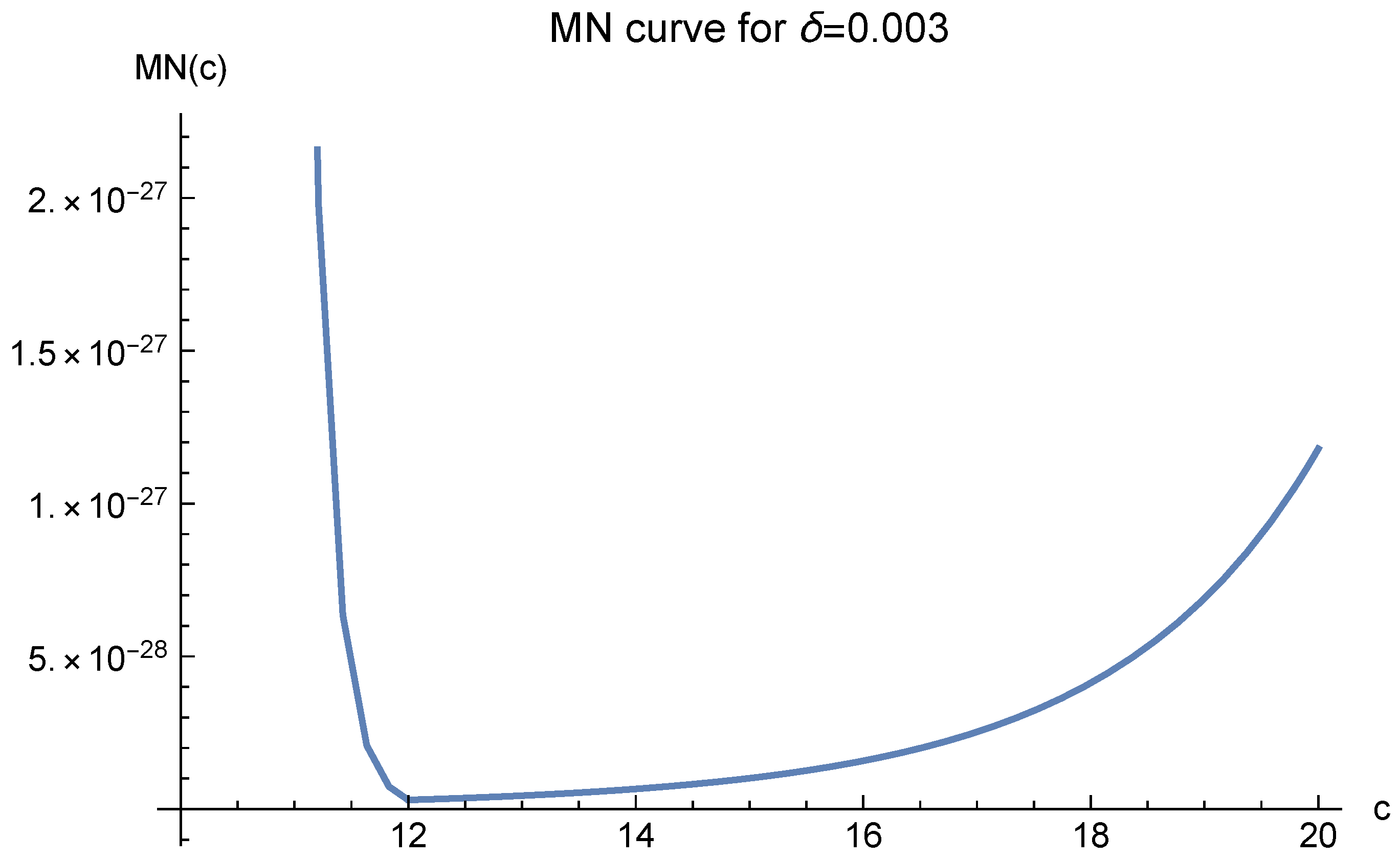
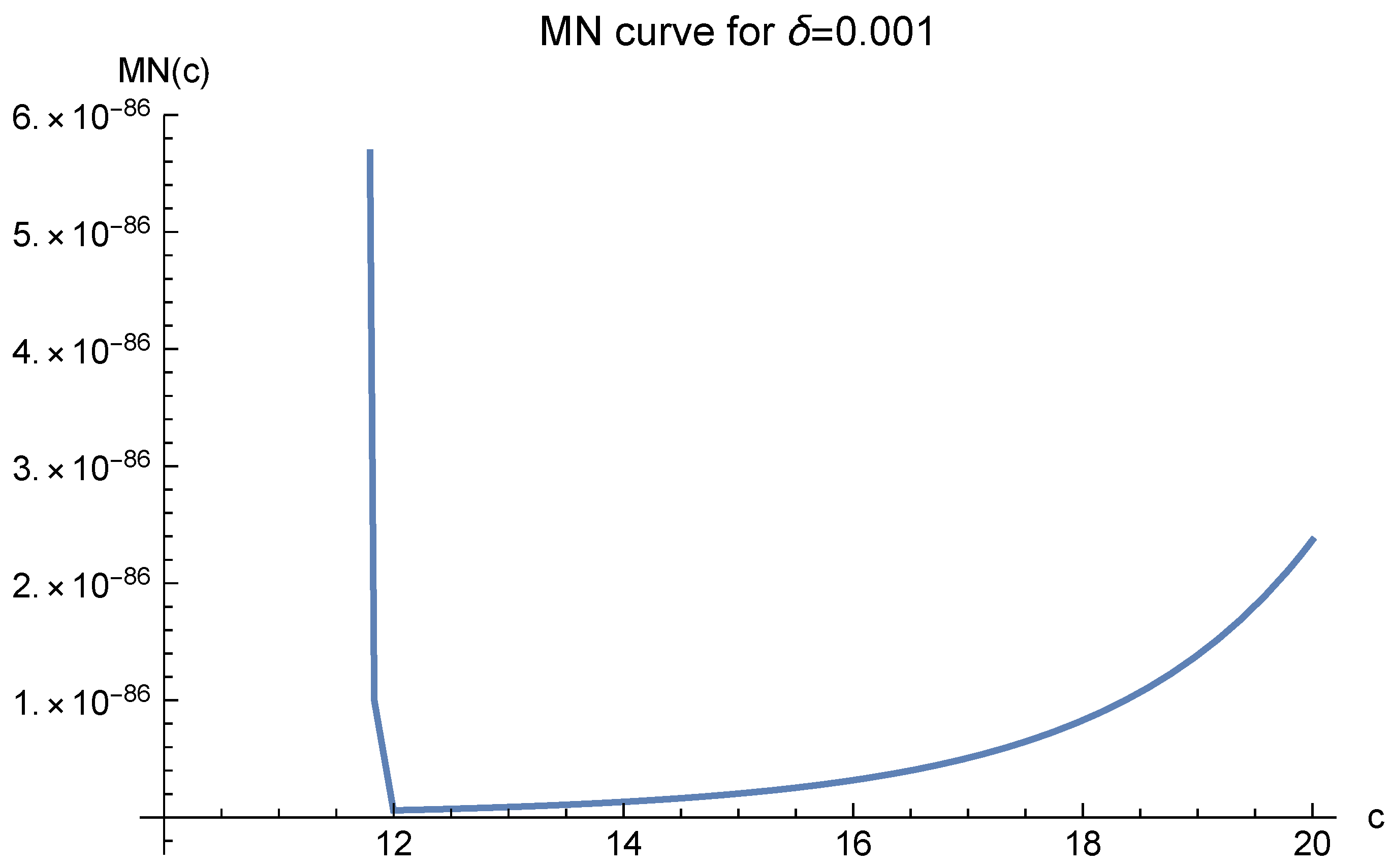
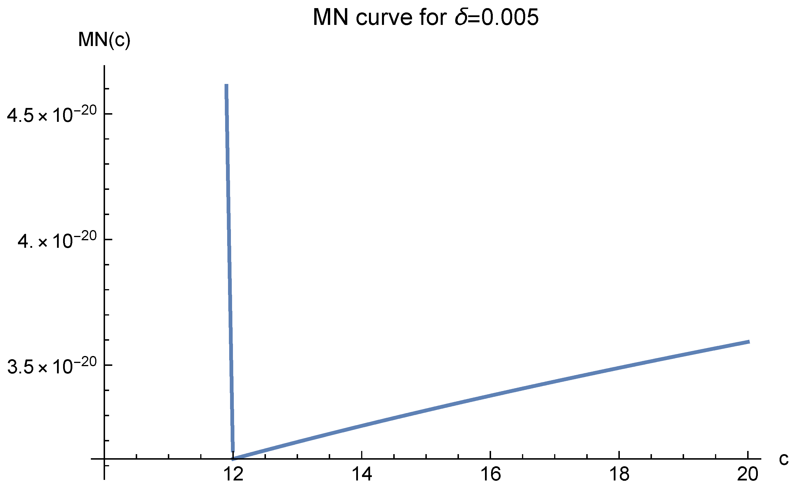
The MN function value greatly depends on the parameter $\sigma$ in the definition of $\mathrm{MN}\left(c\right)$. We present three curves for $\sigma ={10}^{-1}$ and three for $\sigma ={10}^{-5}$ in Figure 1, Figure 2 and Figure 3 and Figure 4, Figure 5 and Figure 6, respectively. In the figures, $\delta$ denotes the fill distance, $b_0$ denotes the domain diameter, d is the dimension, and $\beta$ is the parameter in the definition of the multiquadrics (1).

Note that in these figures, $c=12$ always corresponds to the minimal value of $\mathrm{MN}\left(c\right)$. It suggests that one should choose $c=12$ in our approximate solution to the Poisson equation. We present the experimental results in Table 1. In the table, $N_d$ denotes the number of data points used, and $N_{int}$, $N_{bdy}$ denote the number of interior and boundary data points, respectively. We use $N_t$ test points to measure the quality of the approximation

$$\mathrm{RMS}:=\left\{\right(\sum _{i=1}^{N_t}|u\left(x\right)-\widehat{u}\left(x_i\right){|}^2{)/N_t\}}^{1/2}.$$

As in our previous papers, $b_0$ denotes the diameter of the domain, and COND denotes the condition number of the system of the linear Equation (6).

Table 1. 1D experiment, $c=12,b_0=1,N_t=501$.

$N_d$	7	12	22	42	82
$N_{int}$	5	10	20	40	80
$N_{bdy}$	2	2	2	2	2
RMS	$3.2·{10}^{-6}$	$2.5·{10}^{-11}$	$2.7·{10}^{-24}$	$4.9·{10}^{-52}$	$3.2·{10}^{-127}$
COND	$1.3·{10}^{23}$	$1.4·{10}^{39}$	$6.8·{10}^{69}$	$3.3·{10}^{133}$	$2.0·{10}^{281}$

Table 1. 1D experiment, $c=12,b_0=1,N_t=501$.

$N_d$	7	12	22	42	82
$N_{int}$	5	10	20	40	80
$N_{bdy}$	2	2	2	2	2
RMS	$3.2·{10}^{-6}$	$2.5·{10}^{-11}$	$2.7·{10}^{-24}$	$4.9·{10}^{-52}$	$3.2·{10}^{-127}$
COND	$1.3·{10}^{23}$	$1.4·{10}^{39}$	$6.8·{10}^{69}$	$3.3·{10}^{133}$	$2.0·{10}^{281}$

In order to cope with the problem of ill-conditioning, enough effective digits were adopted for each step of the calculations. For example, for $N_d=82$, we adopted 300 effective digits to the right of the decimal point to handle its huge corresponding condition number. Even so, it took only one second for the computer to solve the linear system. All these were achieved in virtue of the computer software Mathematica.

If c is chosen arbitrarily, say $c=1$, then the RMS will be $4.3·{10}^{-30}$ for $N_d=82$. As for the comparison with other choices of c values, we are not going to present in this subsection for three reasons. Firstly, the results for $c=12$ are already quite good. Secondly, in our theory, the prediction is reliable only when enough data points are used, and then the condition number will be extremely large for $d=1$ and $b_0=1$. For example, experimentally, we found that the optimal value of c is 1600 for $N_d=162$, when $\mathrm{COND}=1.5·{10}^{1211}$ and $\mathrm{RMS}=7.96·{10}^{-359}$. In order to obtain the predicted value $c=12$, we have to increase the number of data points so that $N_d>>162$, as in the experiments for interpolation. Then, the condition number will become much larger than $1.5·{10}^{1211}$, although the RMS will be smaller than $7.96·{10}^{-359}$. In practice we do not need such accuracy. Thirdly, such comparisons can be perfectly handled in the 2D and 3D experiments.

3.2. 2D Model

Our test function is now $u(x,y)=e^{-x-y}$ on $\mathsf{\Omega }=\left\{\right(x,y):0\le x\le 1,0\le y\le 1\}$. This function obviously lies in the Sobolev space. The Poisson equation is then

$$\begin{array}{c}\hfill \left\{\begin{array}{cc}{u}_{xx}(x,y)+u_{yy}(x,y)=2e^{-x-y}\hfill & \mathrm{for} (x,y)\in \mathsf{\Omega }\setminus \partial \mathsf{\Omega },\hfill \\ u(x,y)=g(x,y)\hfill & \mathrm{for} (x,y)\in \partial \mathsf{\Omega },\hfill \end{array}\right.\end{array}$$

(7)

where $g(0,y)=e^{-y},g(x,0)=e^{-x},g(1,y)=e^{-1-y},g(x,1)=e^{-x-1}$ for $0\le x\le 1$ and $0\le y\le 1$.

We are trying to find an approximate solution $\widehat{u}(x,y)={\sum }_{i=1}^N{\lambda }_i\varphi (x-x_i,y-y_i)+{\lambda }_0$, where $\varphi (x,y)=-\sqrt{c^2+x^2+y^2}$ and ${\lambda }_i,i=0,\dots ,N$, are constants to be determined. The sample points $(x_i,y_i),i=1,\dots ,N,$ are scattered in the domain $\mathsf{\Omega }$. Our focus is the choice of c.

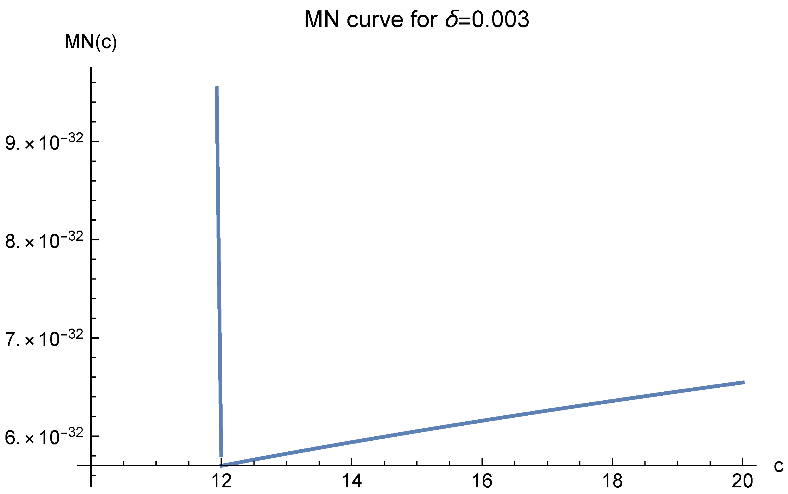
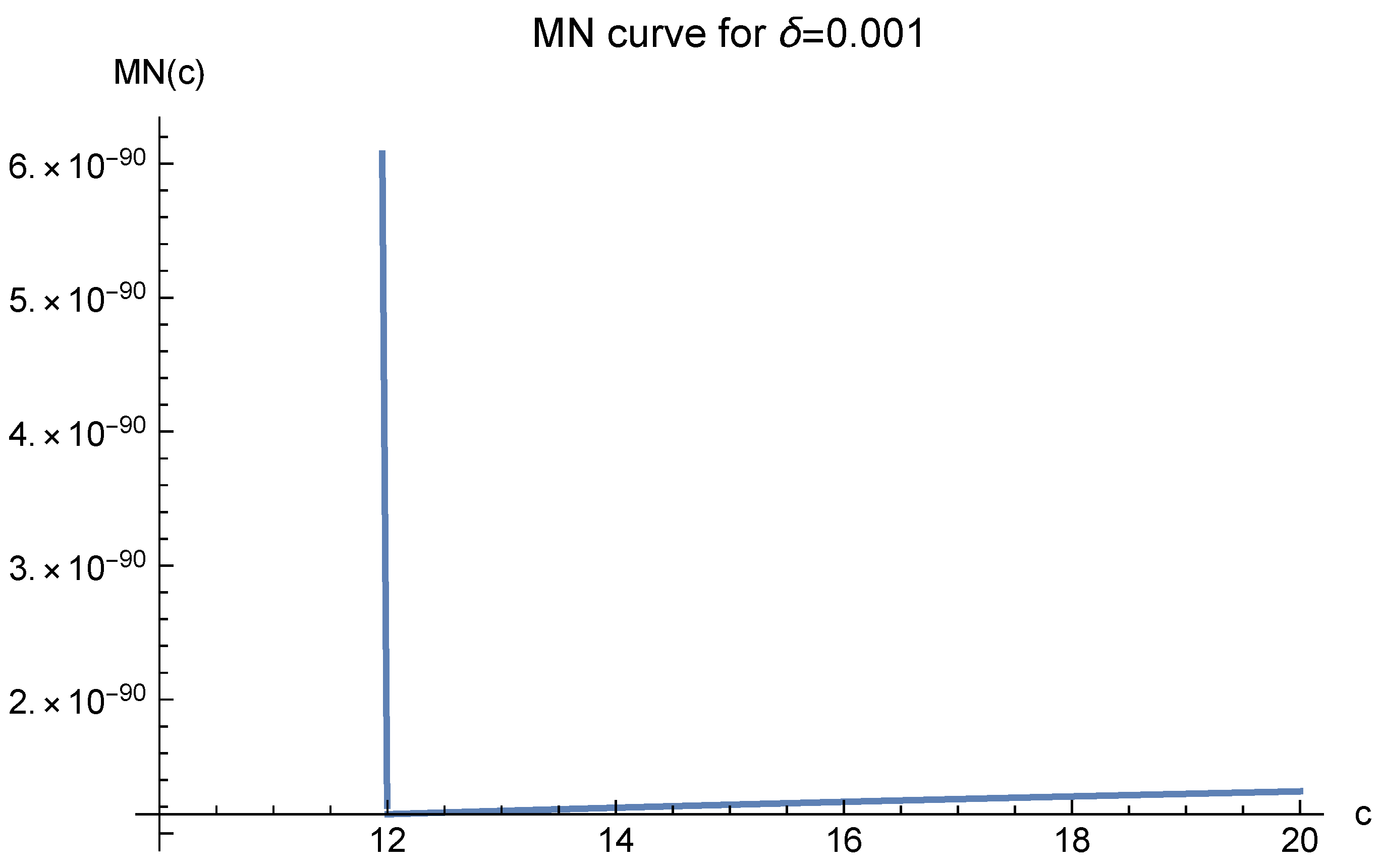
Now, let us analyze the MN curves. We first let $\sigma ={10}^{-1}$ and list five MN curves with different fill distances $\delta$.

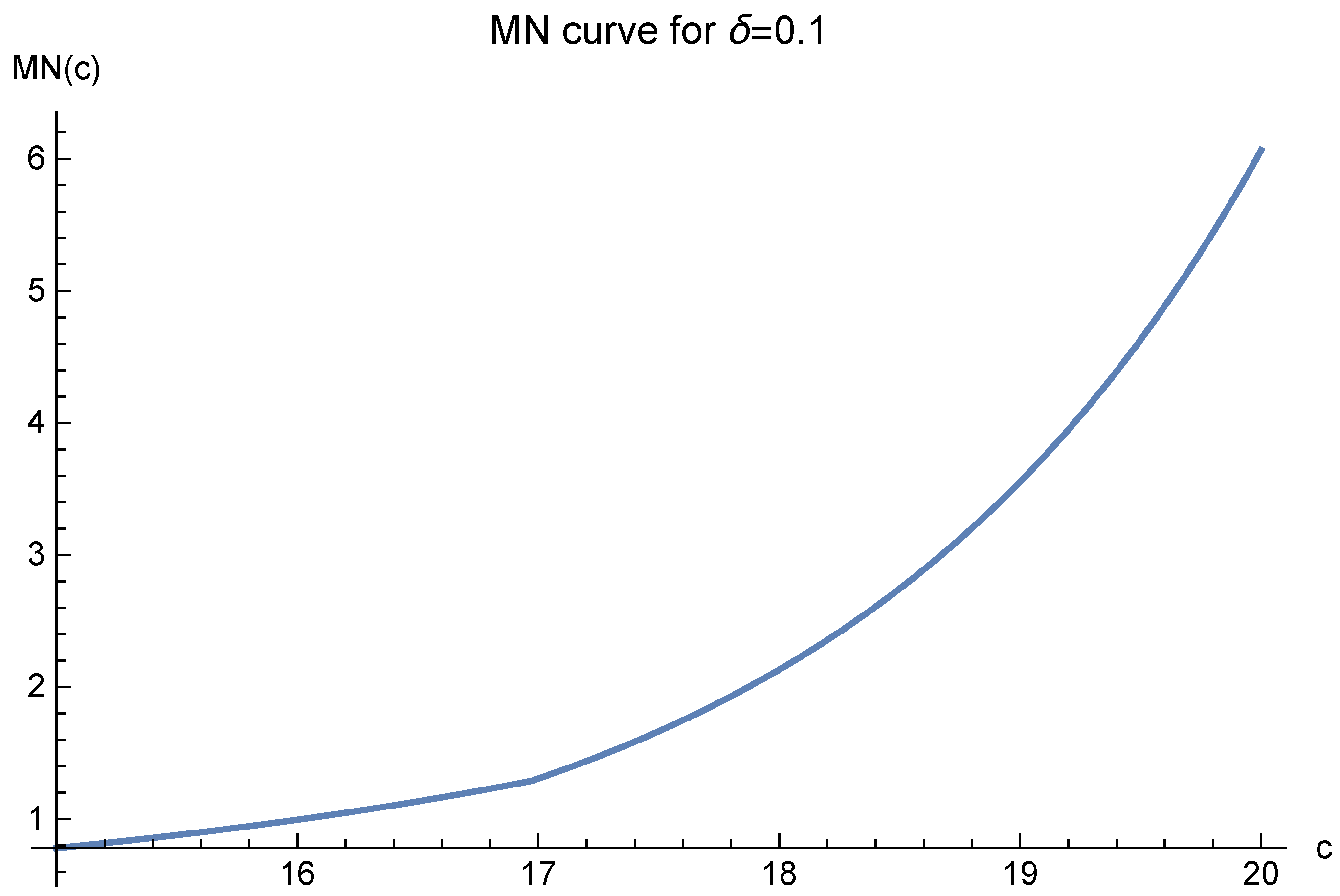
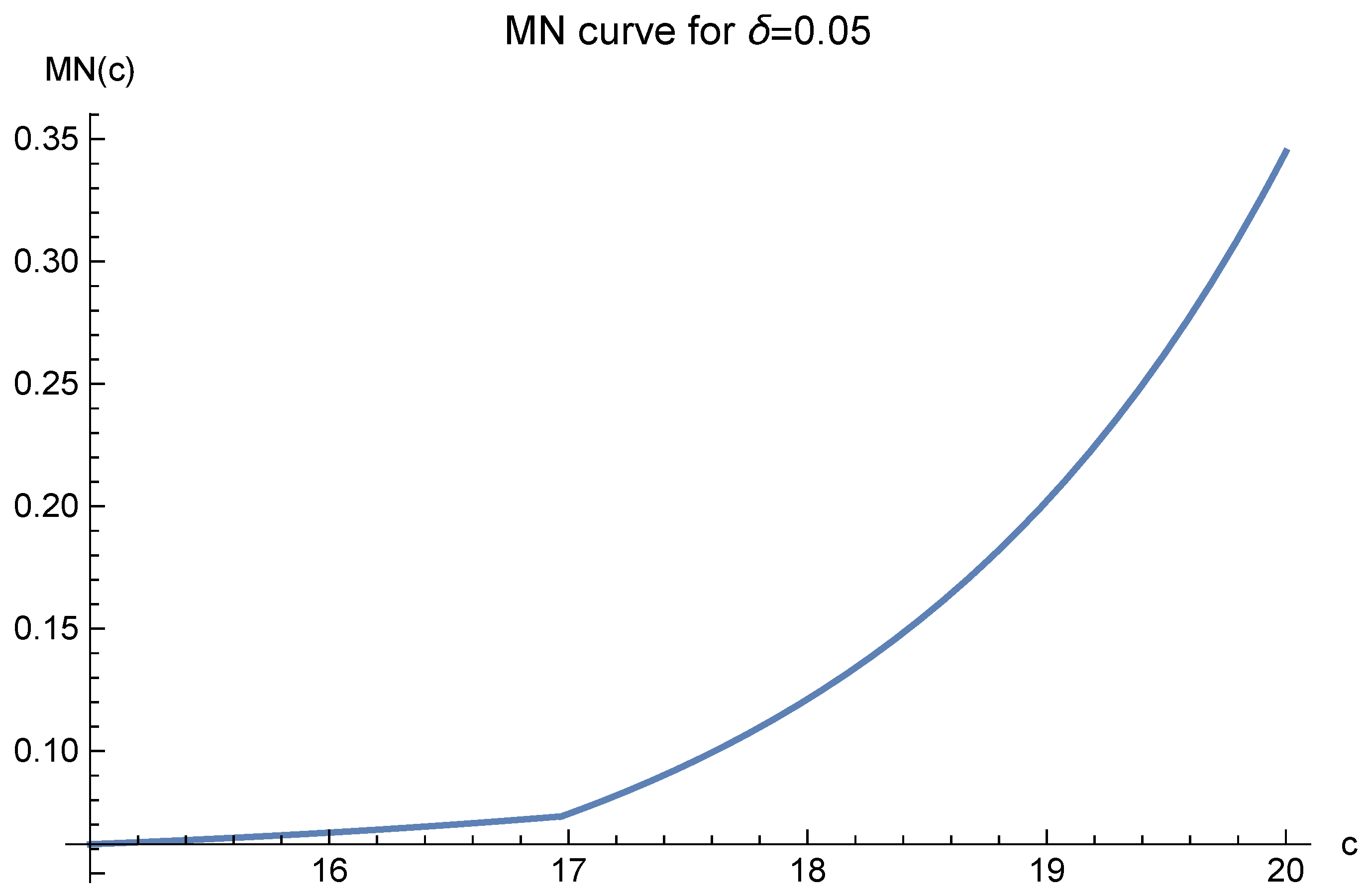
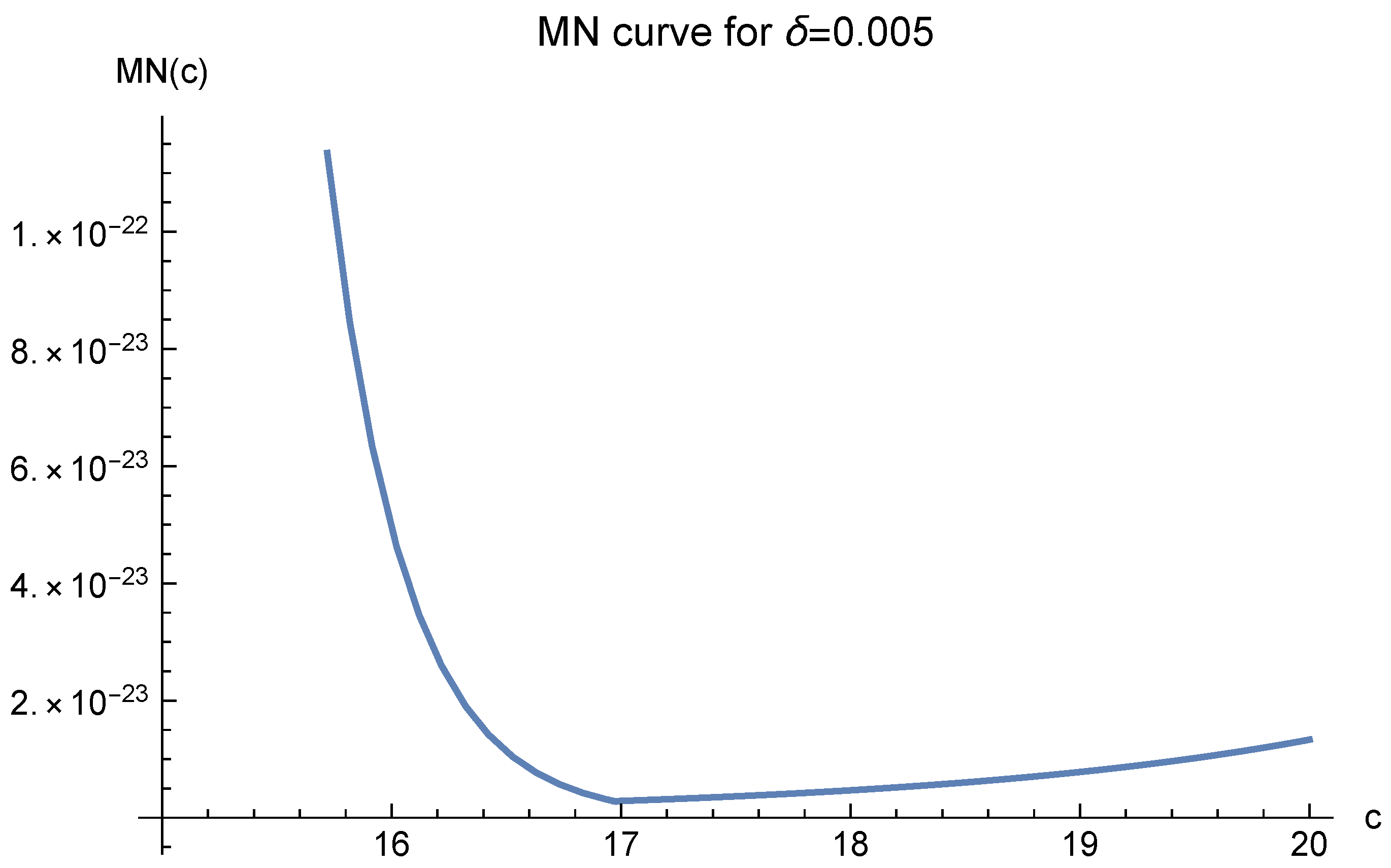
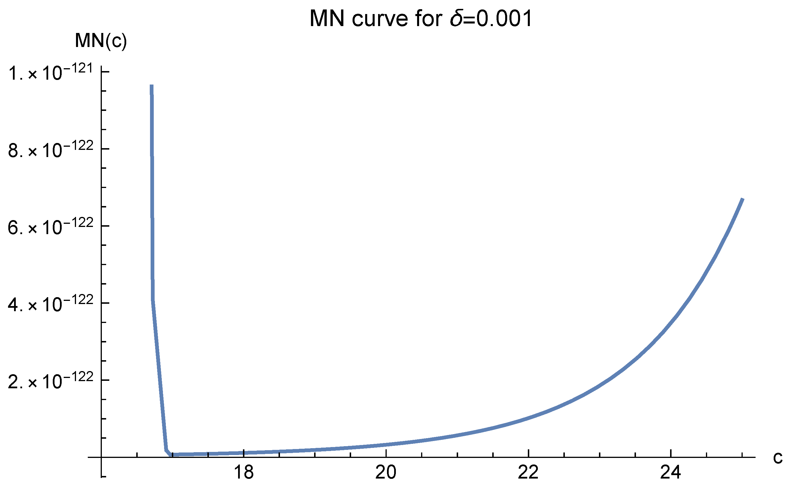
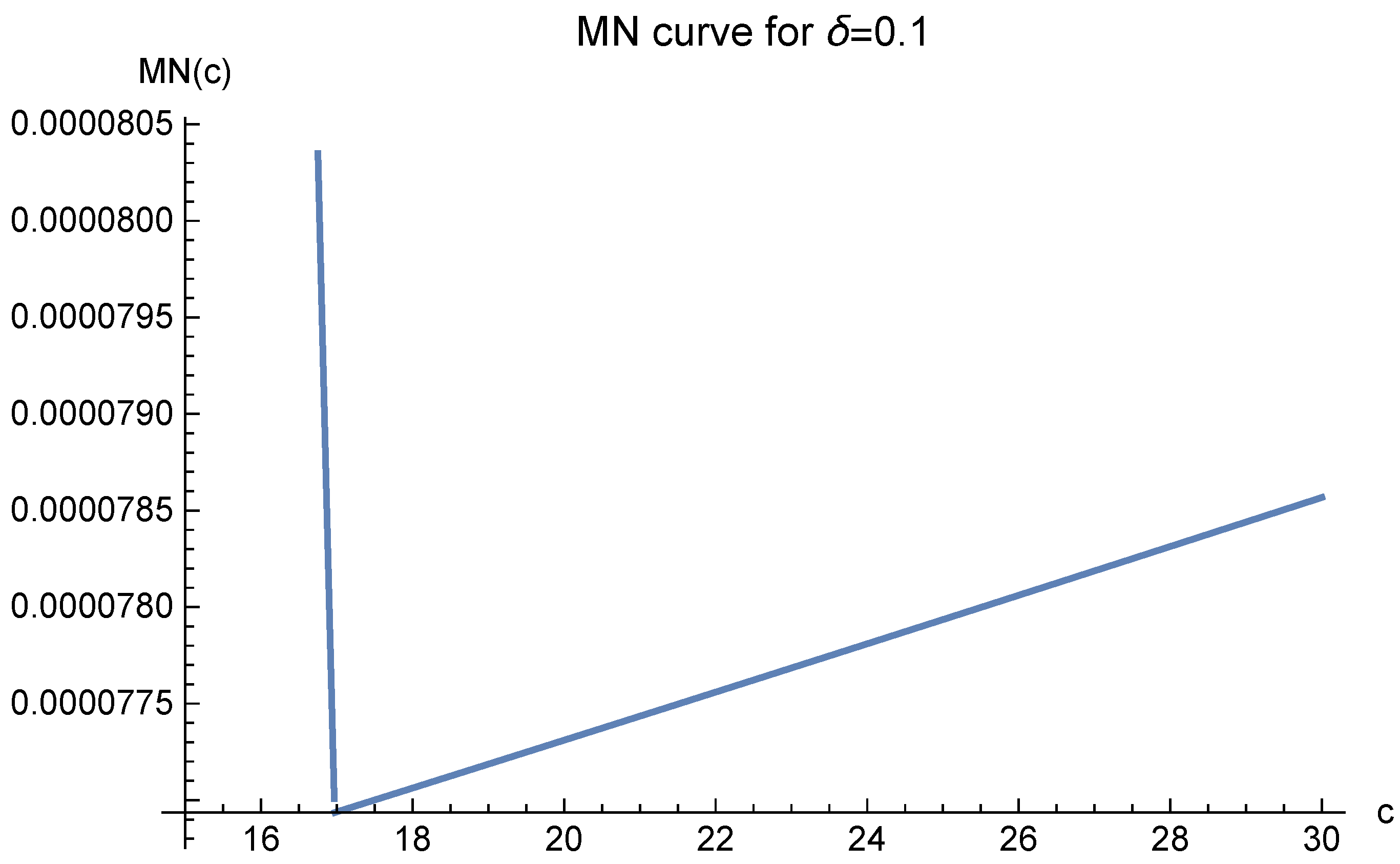
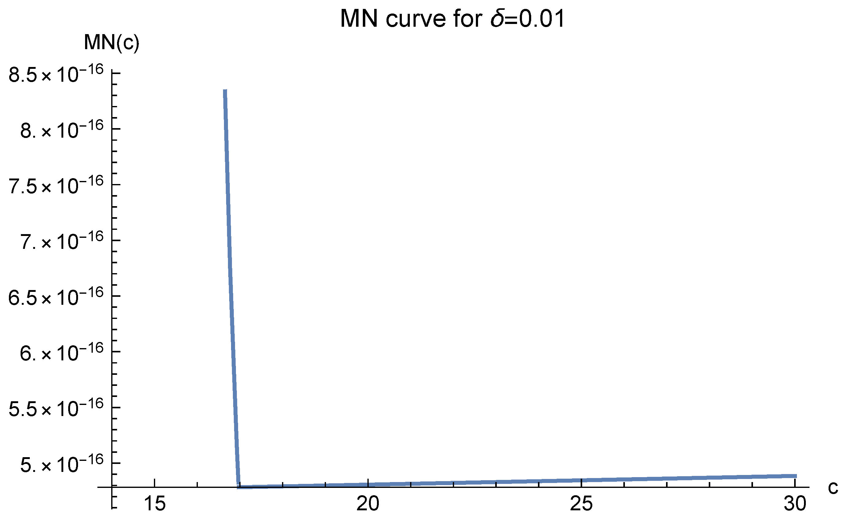
In Figure 7, Figure 8, Figure 9, Figure 10 and Figure 11, it is clearly observed that as the fill distances decrease, the lowest points of the curves move to a fixed value $c=17$ which is just $12b_0\rho$ in Case 3 of the definition of $\mathrm{MN}\left(c\right)$. Now, we investigate $\sigma ={10}^{-5}$.

Figure 12, Figure 13 and Figure 14 also demonstrate that the optimal choice of c is 17. In fact, if we test other $\sigma$’s, the same result will appear. In order to save space, we do not list them.

All the MN curves strongly suggest that one should choose $c=17$ whenever enough data points are used. Thus, we investigate its quality and present the results in Table 2. Here, $N_{bdy}$ and $N_{int}$ denote the numbers of data points located on the boundary and interior of the domain, respectively. Then, $N_d$ and $N_t$ denote the total numbers of data points and test points, respectively. The root-mean-square error, used to measure the approximation error, is defined by

$$\mathrm{RMS}:=\left\{\right(\sum _{i=1}^{N_t}|u(x_i,y_i)-\widehat{u}(x_i,y_i){|}^2{)/N_t\}}^{1/2}.$$

As before, $b_0$ denotes the diameter of the domain $\mathsf{\Omega }$ and COND is the condition number of the linear system involved. The most time-consuming work of solving the linear system took only two seconds for 341 data points. Hence, we did not put the computer time into the table.

Figure 7. MN curve for $\delta =0.1$ where $d=2,\beta =1,b_0=\sqrt{2}$ and $\sigma ={10}^{-1}$.

Figure 7. MN curve for $\delta =0.1$ where $d=2,\beta =1,b_0=\sqrt{2}$ and $\sigma ={10}^{-1}$.

Figure 8. MN curve for $\delta =0.05$ where $d=2,\beta =1,b_0=\sqrt{2}$ and $\sigma ={10}^{-1}$.

Figure 8. MN curve for $\delta =0.05$ where $d=2,\beta =1,b_0=\sqrt{2}$ and $\sigma ={10}^{-1}$.

Figure 9. MN curve for $\delta =0.01$ where $d=2,\beta =1,b_0=\sqrt{2}$ and $\sigma ={10}^{-1}$.

Figure 9. MN curve for $\delta =0.01$ where $d=2,\beta =1,b_0=\sqrt{2}$ and $\sigma ={10}^{-1}$.

Figure 10. MN curve for $\delta =0.005$ where $d=2,\beta =1,b_0=\sqrt{2}$ and $\sigma ={10}^{-1}$.

Figure 10. MN curve for $\delta =0.005$ where $d=2,\beta =1,b_0=\sqrt{2}$ and $\sigma ={10}^{-1}$.

Figure 11. MN curve for $\delta =0.001$ where $d=2,\beta =1,b_0=\sqrt{2}$ and $\sigma ={10}^{-1}$.

Figure 11. MN curve for $\delta =0.001$ where $d=2,\beta =1,b_0=\sqrt{2}$ and $\sigma ={10}^{-1}$.

Figure 12. MN curve for $\delta =0.1$ where $d=2,\beta =1,b_0=\sqrt{2}$ and $\sigma ={10}^{-5}$.

Figure 12. MN curve for $\delta =0.1$ where $d=2,\beta =1,b_0=\sqrt{2}$ and $\sigma ={10}^{-5}$.

Figure 13. MN curve for $\delta =0.01$ where $d=2,\beta =1,b_0=\sqrt{2}$ and $\sigma ={10}^{-5}$.

Figure 13. MN curve for $\delta =0.01$ where $d=2,\beta =1,b_0=\sqrt{2}$ and $\sigma ={10}^{-5}$.

Figure 14. MN curve for $\delta =0.005$ where $d=2,\beta =1,b_0=\sqrt{2}$ and $\sigma ={10}^{-5}$.

Figure 14. MN curve for $\delta =0.005$ where $d=2,\beta =1,b_0=\sqrt{2}$ and $\sigma ={10}^{-5}$.

Table 2. 2D experiment, $c=17,b_0=\sqrt{2},N_t=961$.

$N_d$	46	91	141	191	341
$N_{int}$	5	50	100	150	300
$N_{bdy}$	41	41	41	41	41
RMS	$2.3·{10}^{-5}$	$2.4·{10}^{-12}$	$2.4·{10}^{-16}$	$7.2·{10}^{-20}$	$9.2·{10}^{-25}$
COND	$1.0·{10}^{40}$	$6.5·{10}^{44}$	$5.4·{10}^{53}$	$1.3·{10}^{64}$	$4.8·{10}^{87}$

Table 2. 2D experiment, $c=17,b_0=\sqrt{2},N_t=961$.

$N_d$	46	91	141	191	341
$N_{int}$	5	50	100	150	300
$N_{bdy}$	41	41	41	41	41
RMS	$2.3·{10}^{-5}$	$2.4·{10}^{-12}$	$2.4·{10}^{-16}$	$7.2·{10}^{-20}$	$9.2·{10}^{-25}$
COND	$1.0·{10}^{40}$	$6.5·{10}^{44}$	$5.4·{10}^{53}$	$1.3·{10}^{64}$	$4.8·{10}^{87}$

For simplicity, the test points were evenly spaced in the domain. The interior data points were purely scattered and generated randomly by Mathematica in the domain, but the boundary data points were evenly spaced just for ease of programming. The problem of ill-conditioning was overcome by keeping enough effective digits to the right of the decimal point for each step of the computation. For example, when $N_d=341$, we adopted 200 digits and successfully defeated the large condition number $4.8\times {10}^{87}$. In fact, 110 digits are already good enough and will lead to the same result. Even with 200 digits, it took only two seconds to solve the linear system. All these were achieved by the help of the arbitrarily precise computer software Mathematica.

Although $c=17$ leads to satisfactory results, a comparison with other choices of c is also needed.

Table 3. 2D experiment, $b_0=\sqrt{2},N_d=341,N_t=961$.

c	1	10	17	30	50
RMS	$1.1·{10}^{-8}$	$5.2·{10}^{-22}$	$9.2·{10}^{-25}$	$1.4·{10}^{-24}$	$4.1·{10}^{-24}$
COND	$1.8·{10}^{28}$	$7.0·{10}^{75}$	$4.8·{10}^{87}$	$1.6·{10}^{100}$	$2.0·{10}^{111}$
c	70	90	110	130	150
RMS	$2.2·{10}^{-23}$	$2.4·{10}^{-22}$	$3.2·{10}^{-22}$	$2.8·{10}^{-22}$	$3.6·{10}^{-22}$
COND	$1.2·{10}^{119}$	$1.8·{10}^{125}$	$2.9·{10}^{129}$	$5.9·{10}^{132}$	$5.8·{10}^{135}$

offers such a comparison. We fix $N_{int}=300$ and $N_{bdy}=41$ for all choices of c.

In Table 3, it is clear that our theoretically predicted optimal value $c=17$ coincides exactly with the experimentally optimal value. Moreover, as depicted by the MN curves in Figure 12, Figure 13 and Figure 14, the approximation errors become large very slowly for $c>17$. This is fully reflected by our experimental results.

The three-dimensional experiment is more challenging and is expected to be much more time-consuming. Fortunately, it takes only five minutes to compute the linear system, as we shall see in the next subsection.

3.3. 3D Model

The test function is now $u(x,y,z)=e^{-x-y-z}$ on $\mathsf{\Omega }=\left\{\right(x,y,z):0\le x\le 1,$$0\le y\le 1,$$0\le z\le 1\}$. It lies in the Sobolev space. The Poisson equation is

$$\begin{array}{c}\hfill \left\{\begin{array}{cc}{u}_{xx}(x,y,z)+u_{yy}(x,y,z)+u_{zz}(x,y,z)=3e^{-x-y-z}\hfill & \mathrm{for} (x,y,z)\in \mathsf{\Omega }\setminus \partial \mathsf{\Omega },\hfill \\ u(x,y,z)=g(x,y,z)\hfill & \mathrm{for} (x,y,z)\in \partial \mathsf{\Omega },\hfill \end{array}\right.\end{array}$$

(8)

where $g(x,y,z)$ is just the restriction of $u(x,y,z)$ to the six surfaces of the domain cube. In other words, the Dirichlet condition is adopted.

The approximate solution will be of the form $\widehat{u}(x,y,z)={\sum }_{i=1}^N{\lambda }_i\varphi (x-x_i,y-y_i,z-z_i)+{\lambda }_0$ where $\varphi (x,y,z)=-\sqrt{c^2+x^2+y^2+z^2}$ and ${\lambda }_i,i=0,\dots ,N$, are constants to be determined. The sample points $(x_i,y_i,z_i),i=1,\dots ,N$, are still scattered in the interior of the domain cube and evenly spaced on the boundary. We are going to find c such that the approximation error $|u(x,y,z)-\widehat{u}(x,y,z)|$ is as small as possible.

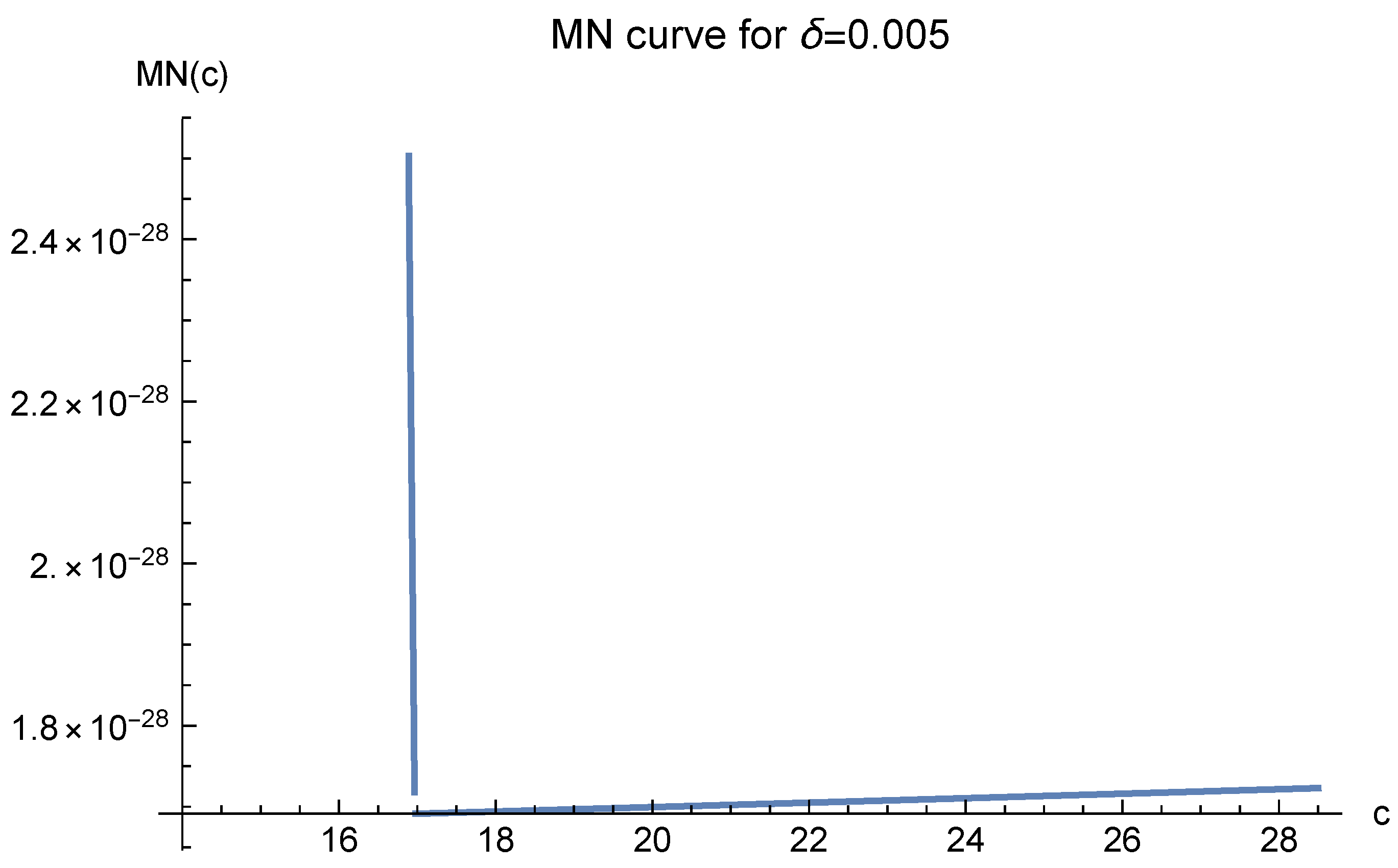
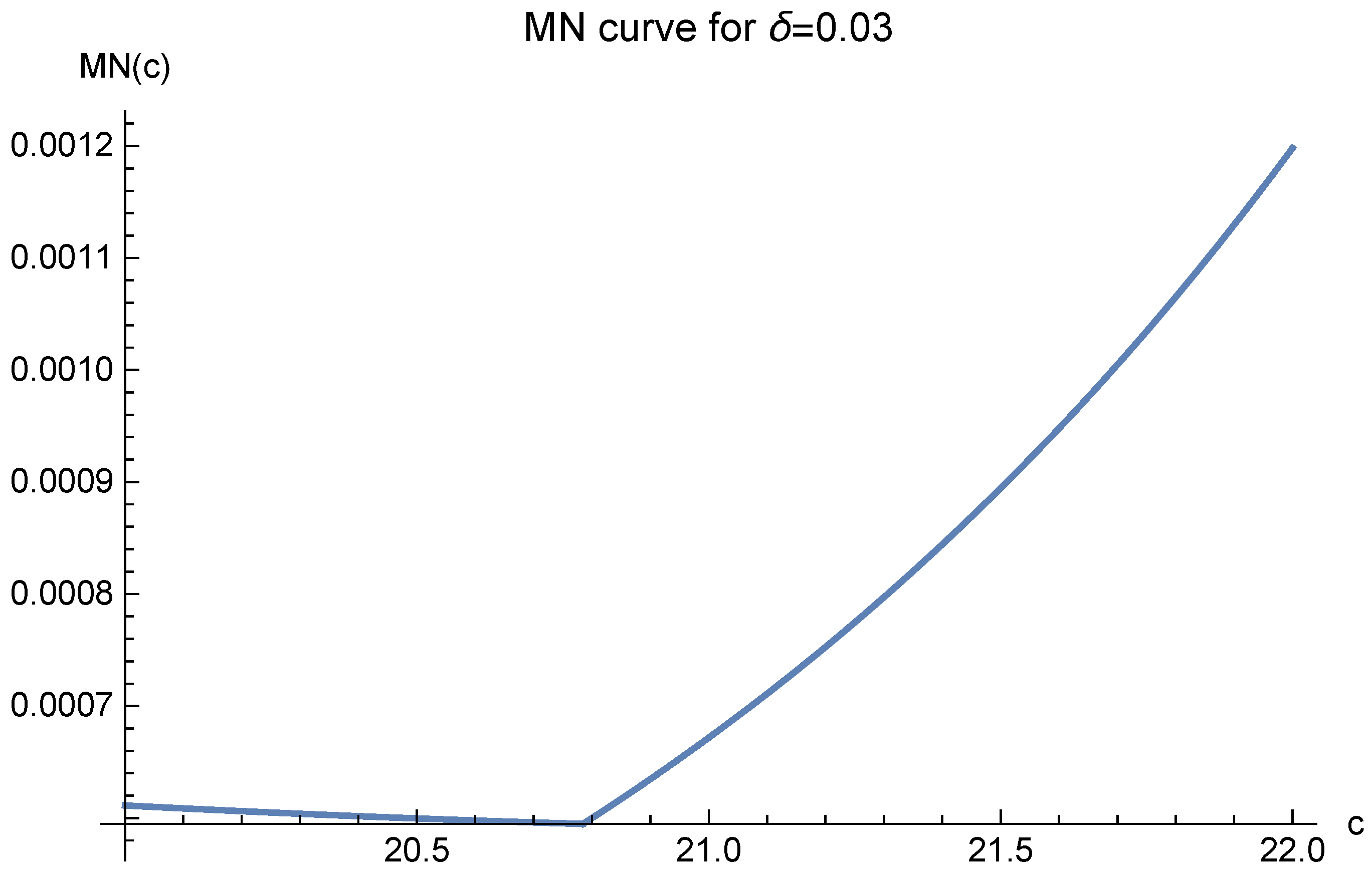
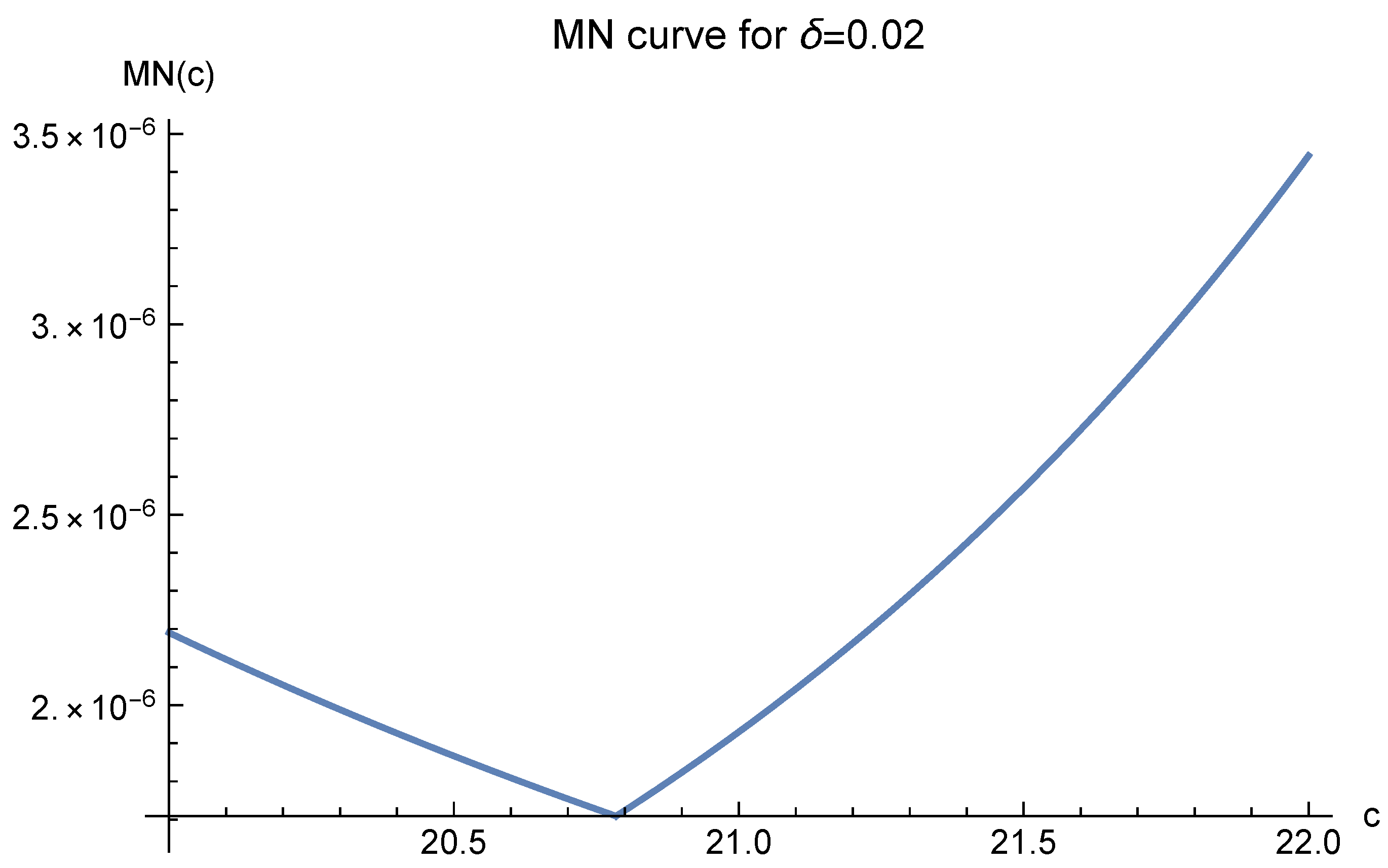
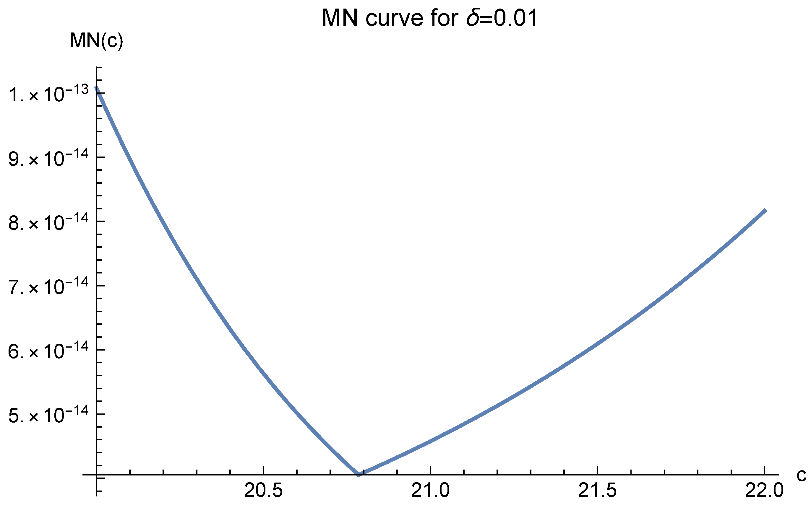
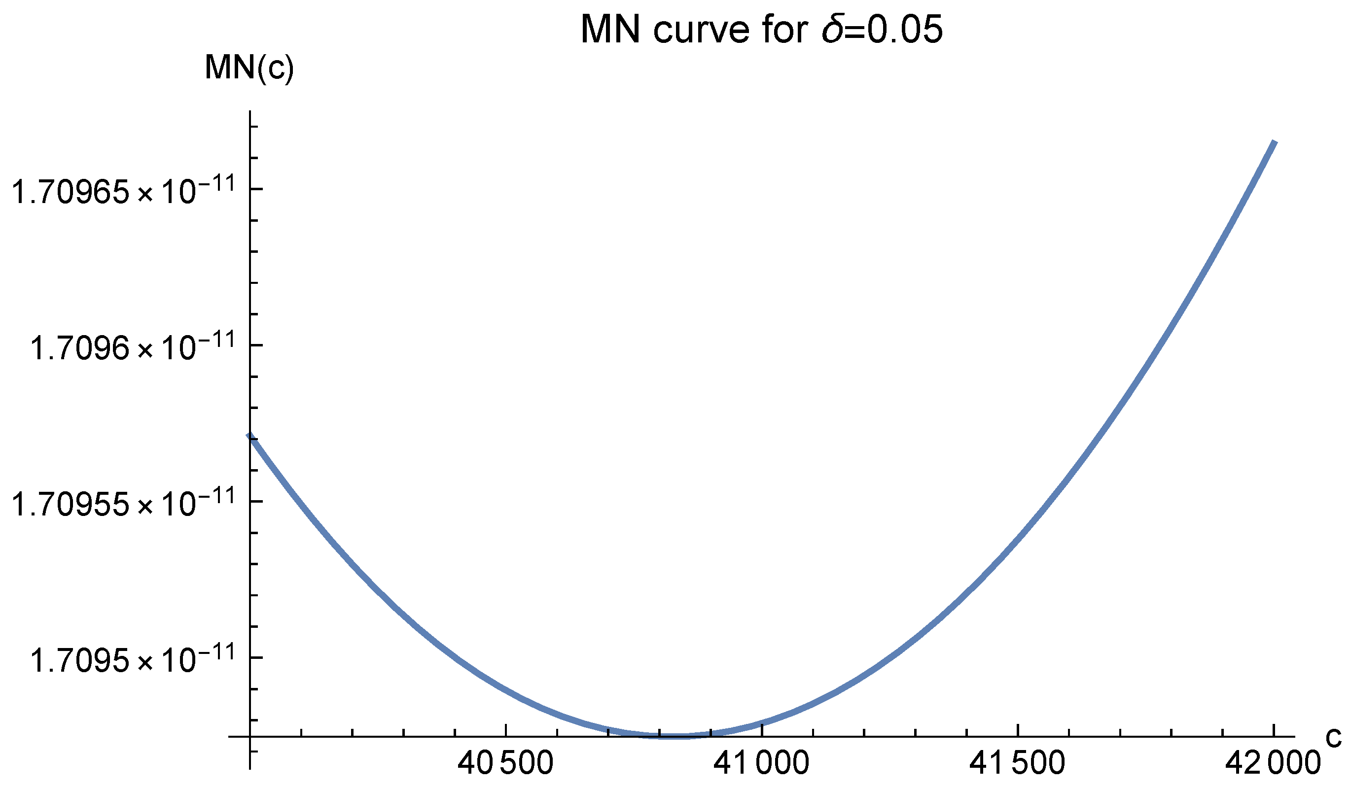
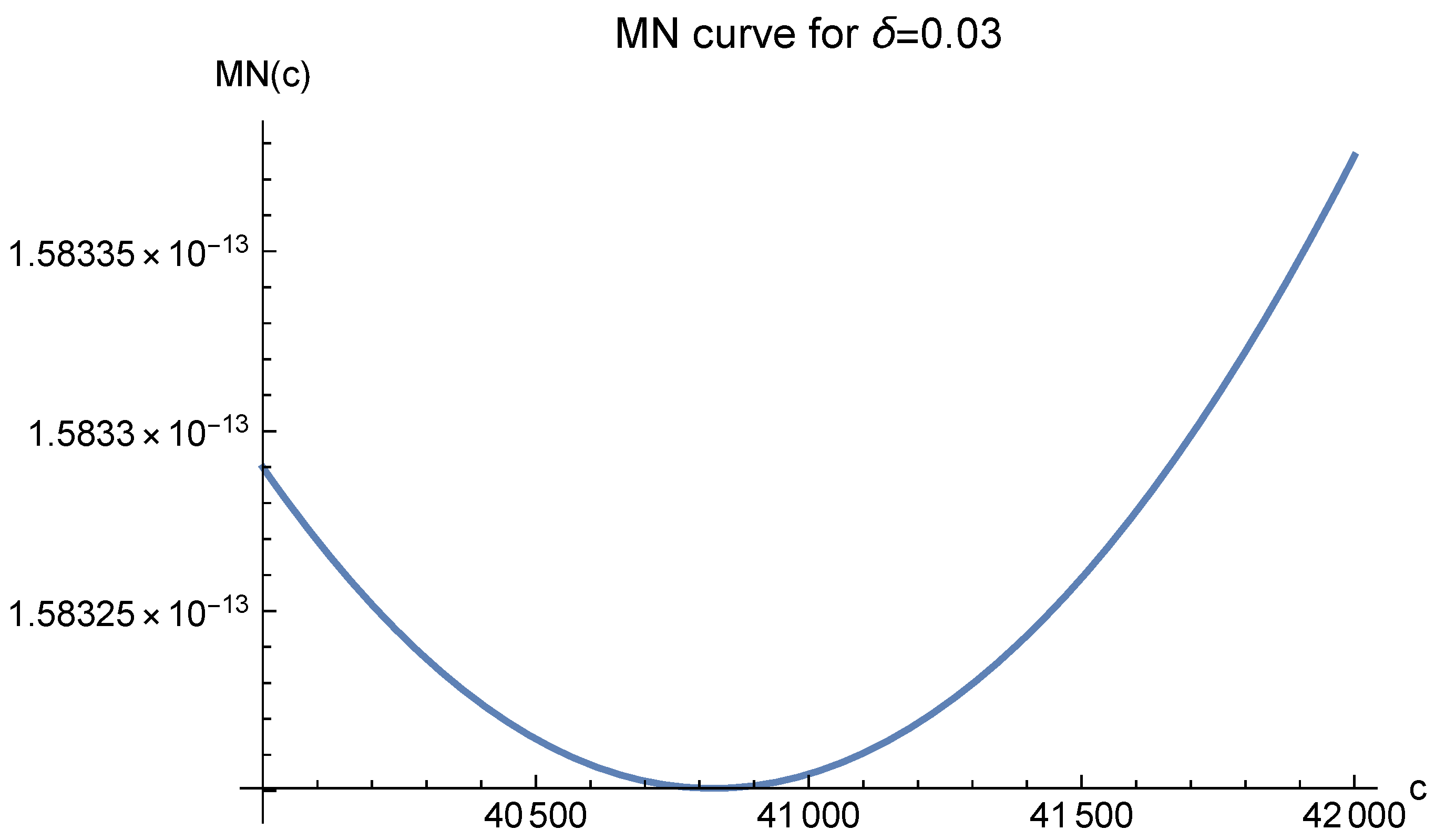
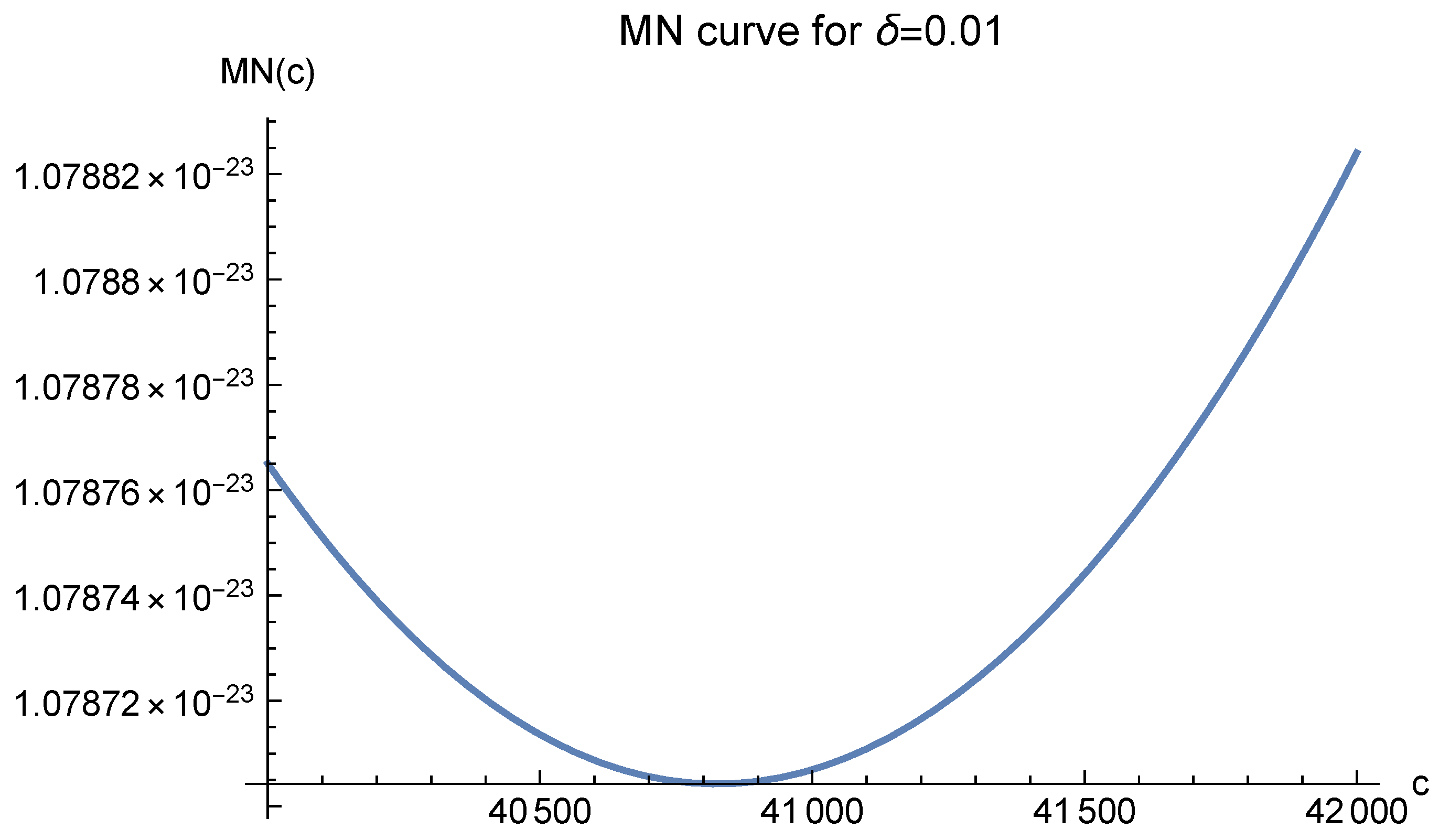
In order to find a suitable c, one has to analyze the MN curves first. Again, Case 3 of $\mathrm{MN}\left(c\right)$ applies. However, for 3D MN functions, different $\sigma$’s indicate different optimal values of c. For $\sigma ={10}^{-1}$, the optimal values of c are shown in Figure 15, Figure 16, Figure 17, Figure 18 and Figure 19. These figures show that as long as $\delta$ is small enough, the optimal value of c is 20.7846, which is just $12b_0\rho$ in the definition of $\mathrm{MN}\left(c\right)$.

Now, we test $\sigma ={10}^{-5}$. The MN curves are presented in Figure 20, Figure 21 and Figure 22. They demonstrate that one should choose $c=129$.

The MN curves for $\sigma ={10}^{-10}$ are as in Figure 23, Figure 24 and Figure 25. They indicate that one should let c = 40,800.

The three different optimal values of c are all logically correct. However, when $\sigma$ is very small, ${\parallel f\parallel }_{E_{\sigma }}$ in (4) will be extremely large, making (4) meaningless. Hence, we should choose $c=20.7846$ according to Figure 15, Figure 16, Figure 17, Figure 18 and Figure 19, where $\sigma ={10}^{-1}$ is larger and the $\mathrm{MN}\left(c\right)$ values are reasonably small.

For $c=20.7846$, we compare different numbers of data points. The results are presented in Table 4.

Figure 15. MN curve for $\delta =0.05$ where $d=3,\beta =1,b_0=\sqrt{3}$ and $\sigma ={10}^{-1}$.

Figure 15. MN curve for $\delta =0.05$ where $d=3,\beta =1,b_0=\sqrt{3}$ and $\sigma ={10}^{-1}$.

Figure 16. MN curve for $\delta =0.03$ where $d=3,\beta =1,b_0=\sqrt{3}$ and $\sigma ={10}^{-1}$.

Figure 16. MN curve for $\delta =0.03$ where $d=3,\beta =1,b_0=\sqrt{3}$ and $\sigma ={10}^{-1}$.

Figure 17. MN curve for $\delta =0.02$ where $d=3,\beta =1,b_0=\sqrt{3}$ and $\sigma ={10}^{-1}$.

Figure 17. MN curve for $\delta =0.02$ where $d=3,\beta =1,b_0=\sqrt{3}$ and $\sigma ={10}^{-1}$.

Figure 18. MN curve for $\delta =0.01$ where $d=3,\beta =1,b_0=\sqrt{3}$ and $\sigma ={10}^{-1}$.

Figure 18. MN curve for $\delta =0.01$ where $d=3,\beta =1,b_0=\sqrt{3}$ and $\sigma ={10}^{-1}$.

Figure 19. MN curve for $\delta =0.001$ where $d=3,\beta =1,b_0=\sqrt{3}$ and $\sigma ={10}^{-1}$.

Figure 19. MN curve for $\delta =0.001$ where $d=3,\beta =1,b_0=\sqrt{3}$ and $\sigma ={10}^{-1}$.

Figure 20. MN curve for $\delta =0.05$ where $d=3,\beta =1,b_0=\sqrt{3}$ and $\sigma ={10}^{-5}$.

Figure 20. MN curve for $\delta =0.05$ where $d=3,\beta =1,b_0=\sqrt{3}$ and $\sigma ={10}^{-5}$.

Figure 21. MN curve for $\delta =0.03$ where $d=3,\beta =1,b_0=\sqrt{3}$ and $\sigma ={10}^{-5}$.

Figure 21. MN curve for $\delta =0.03$ where $d=3,\beta =1,b_0=\sqrt{3}$ and $\sigma ={10}^{-5}$.

Figure 22. MN curve for $\delta =0.01$ where $d=3,\beta =1,b_0=\sqrt{3}$ and $\sigma ={10}^{-5}$.

Figure 22. MN curve for $\delta =0.01$ where $d=3,\beta =1,b_0=\sqrt{3}$ and $\sigma ={10}^{-5}$.

Figure 23. MN curve for $\delta =0.05$ where $d=3,\beta =1,b_0=\sqrt{3}$ and $\sigma ={10}^{-10}$.

Figure 23. MN curve for $\delta =0.05$ where $d=3,\beta =1,b_0=\sqrt{3}$ and $\sigma ={10}^{-10}$.

Figure 24. MN curve for $\delta =0.03$ where $d=3,\beta =1,b_0=\sqrt{3}$ and $\sigma ={10}^{-10}$.

Figure 24. MN curve for $\delta =0.03$ where $d=3,\beta =1,b_0=\sqrt{3}$ and $\sigma ={10}^{-10}$.

Figure 25. MN curve for $\delta =0.01$ where $d=3,\beta =1,b_0=\sqrt{3}$ and $\sigma ={10}^{-10}$.

Figure 25. MN curve for $\delta =0.01$ where $d=3,\beta =1,b_0=\sqrt{3}$ and $\sigma ={10}^{-10}$.

Table 4. 3D experiment, $c=20.7846,b_0=\sqrt{3}$.

$N_d$	616	666	766	966	1366
$N_{int}$	50	100	200	400	800
$N_{bdy}$	566	566	566	566	566
$N_t$	1200	1200	1200	1200	1800
RMS	$6.7·{10}^{-9}$	$1.5·{10}^{-11}$	$3.1·{10}^{-13}$	$1.8·{10}^{-15}$	$7.0·{10}^{-19}$
COND	$2.4·{10}^{71}$	$2.6·{10}^{71}$	$3.0·{10}^{71}$	$3.7·{10}^{71}$	$5.5·{10}^{71}$

Table 4. 3D experiment, $c=20.7846,b_0=\sqrt{3}$.

$N_d$	616	666	766	966	1366
$N_{int}$	50	100	200	400	800
$N_{bdy}$	566	566	566	566	566
$N_t$	1200	1200	1200	1200	1800
RMS	$6.7·{10}^{-9}$	$1.5·{10}^{-11}$	$3.1·{10}^{-13}$	$1.8·{10}^{-15}$	$7.0·{10}^{-19}$
COND	$2.4·{10}^{71}$	$2.6·{10}^{71}$	$3.0·{10}^{71}$	$3.7·{10}^{71}$	$5.5·{10}^{71}$

The computation is very efficient. Even though we adopted 200 effective digits for each step of the calculations, the most time-consuming work of solving the linear system took only two seconds for $N_d=616$ and five minutes for $N_d=1366$. In fact, keeping only 100 effective digits would have obtained the same RMS’s and COND’s. We stopped adding more data points at $N_d=1366$ because the RMS is already good enough.

The comparison among different values of c is presented in

Table 5. 3D experiment, $b_0=\sqrt{3},N_d=1366,N_t=1800$.

c	1	15	$20.7846$	30	40
RMS	$8.7·{10}^{-7}$	$2.6·{10}^{-7}$	$7.0·{10}^{-19}$	$7.6·{10}^{-18}$	$1.0·{10}^{-19}$
COND	$4.6·{10}^{21}$	$6.4·{10}^{65}$	$5.5·{10}^{71}$	$2.5·{10}^{78}$	$4.7·{10}^{83}$
c	60	80	100	120	140
RMS	$3.4·{10}^{-19}$	$8.7·{10}^{-19}$	$6.8·{10}^{-19}$	$1.4·{10}^{-19}$	$3.8·{10}^{-19}$
COND	$1.1·{10}^{91}$	$1.9·{10}^{96}$	$2.5·{10}^{100}$	$5.1·{10}^{103}$	$3.2·{10}^{106}$
c	180	220
RMS	$1.7·{10}^{-18}$	$3.7·{10}^{-19}$
COND	$1.2·{10}^{111}$	$5.6·{10}^{114}$

. We fixed $N_d=1366$, $N_{int}=800$ and $N_{bdy}=566$. In order to cope with the problem of ill-conditioning, enough effective digits were adopted for the calculations. For $c=1$, we used 50 digits, and for $c=220$, 140 digits were used. The most time-consuming work of solving the linear system always took less than six minutes’ computer time.

Note that Figure 15, Figure 16, Figure 17, Figure 18 and Figure 19 show that if $\delta$ is small enough, or, equivalently, if the number of data points is large enough, the values of MN(c) become large very slowly for $c>20.7846$. Numerical investigations also demonstrate this. Figure 20, Figure 21, Figure 22, Figure 23, Figure 24 and Figure 25 even tend to move the optimal value of c to the right. All these are supported by the RMS’s in Table 5. Although for $c>20.7846$, the choice of c does not influence the approximation error much, one still has to choose $c=20.7846$ because its corresponding condition number is smaller. In other words, the theoretically predicted optimal value of c coincides with the experimentally optimal one.

4. Discussion

In our experiments, the exact solution function $u(x_1,\dots ,x_d)$ is a natural function contained in the Sobolev space $W_2^{\tau }(R^d)$ for any $\tau \ge 0$. An approximate solution function $\widehat{u}(x_1,\dots ,x_d)$ could always be efficiently found with a very small approximation error. The optimality of our choice of the shape parameter c has also been corroborated. It means that, in the process of the RBF collocation method, any differential equation may be effectively handled by our approach, as long as its solution belongs to Sobolev space, such as the Poisson equation in our experiment. This is exciting. However, how to apply our approach to solving various important but hard differential equations is still very challenging, especially when the solution does not lie in the Sobolev space.

References

1. Wendland, H. Scattered Data Approximation; Cambridge University Press: Cambridge, UK, 2005. [Google Scholar]
2. Kansa, E.J. Multiquadrics—A Scattered data approximation scheme with applications to computational fluid dynamics I: Surface approximations and partial derivative estimates. Comput. Math. Appl. 1990, 19, 127–145. [Google Scholar] [CrossRef] [Green Version]
3. Kansa, E.J. Multiquadrics—A scattered data approximation scheme with applications to computational fluid dynamics II:Solutions to parabolic, hyperbolic, and elliptic partial differential equations. Comput. Math. Appl. 1990, 19, 147–161. [Google Scholar] [CrossRef] [Green Version]
4. Fasshauer, G. Meshfree Approximation Methods with MATLAB; World Scientific Publishers: Singapore, 2007. [Google Scholar]
5. Yosida, K. Functional Analysis; Springer: Berlin/Heidelberg, Germany, 1980. [Google Scholar]
6. Narcowich, F.J.; Ward, J.D.; Wendland, H. Sobolev error estimates and a Berstein inequality for scattered data interpolation via radial basis functions. Constr. Approx. 2006, 20, 175–186. [Google Scholar] [CrossRef]
7. Luh, L.-T. The mystery of the shape parameter IV. Eng. Anal. Bound. Elem. 2014, 48, 24–31. [Google Scholar] [CrossRef] [Green Version]
8. Luh, L.-T. The choice of the shape parameter-a friendly approach. Eng. Anal. Bound. Elem. 2019, 98, 103–109. [Google Scholar] [CrossRef]
Figure 1. MN curve for δ = 0.005 where d = 1 , β = 1 , b 0 = 1 and σ = 10 1 .
Mathematics 10 03583 g001
Figure 2. MN curve for δ = 0.003 where d = 1 , β = 1 , b 0 = 1 and σ = 10 1 .
Mathematics 10 03583 g002
Figure 3. MN curve for δ = 0.001 where d = 1 , β = 1 , b 0 = 1 and σ = 10 1 .
Mathematics 10 03583 g003
Figure 4. MN curve for δ = 0.005 where d = 1 , β = 1 , b 0 = 1 and σ = 10 5 .
Mathematics 10 03583 g004
Figure 5. MN curve for δ = 0.003 where d = 1 , β = 1 , b 0 = 1 and σ = 10 5 .
Mathematics 10 03583 g005
Figure 6. MN curve for δ = 0.001 where d = 1 , β = 1 , b 0 = 1 and σ = 10 5 .
Mathematics 10 03583 g006