A Collocation Method for Mixed Volterra–Fredholm Integral Equations of the Hammerstein Type

Abstract

This paper presents a collocation method for the approximate solution of two-dimensional mixed Volterra–Fredholm integral equations of the Hammerstein type. For a reformulation of the equation, we consider the domain of integration as a planar triangle and use a special type of linear interpolation on triangles. The resulting quadrature formula has a higher degree of precision than expected, leading to a collocation method that is superconvergent at the collocation nodes. The convergence of the method is established, as well as the rate of convergence. Numerical examples are considered, showing the applicability of the proposed scheme and the agreement with the theoretical results.

1. Introduction

Integral equations are an important part of applied mathematics, as they have various applications in physics, engineering, biology, hydrodynamics, thermodynamics, etc. They also provide mathematical models for the progress of an epidemic and many other physical and biological problems (see [1]).

They have been studied extensively, both theoretically (existence, uniqueness, stability, data dependence of the solution) and numerically. Numerical solutions have been found using Adomian decomposition [2], Nyström methods [3,4], collocation [5,6,7], block-pulse functions [8], Gaussian quadratures [9], iterative methods [10,11], etc. To approximate solutions, a wide variety of functions have been employed, such as wavelets [12,13,14], Taylor series expansions [15], quasi-interpolating projectors [16], Bernoulli polynomials [17], and others. In this paper, we investigate a collocation method based on piecewise linear interpolation over triangles.

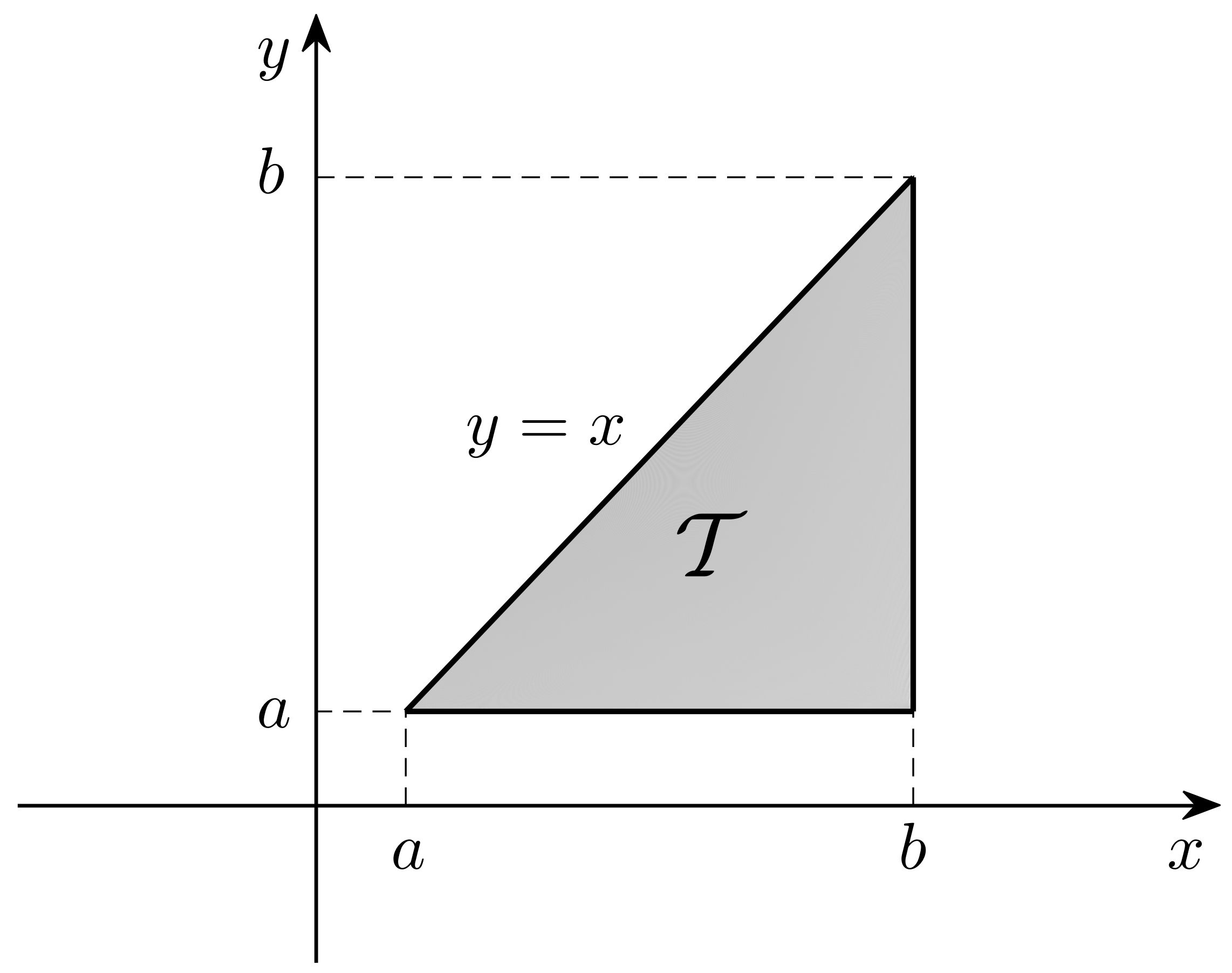
A mixed Volterra–Fredholm integral equation (MVFIE) is an integral equation of the type

$$u(x,y)=\underset{a}{\overset{x}{{\displaystyle \int }}}\underset{\mathsf{\Omega }}{\int }K\left(x,y,\xi ,\eta ,u(\xi ,\eta )\right)d\xi d\eta +f(x,y),(x,y)\in [a,b]\times \mathsf{\Omega },$$

where $\mathsf{\Omega }$ is a closed bounded subset of ${\mathbb{R}}^n,n=1,2,3.$ Such equations arise in integral reformulations of various initial and boundary value problems for partial differential equations in heat and fluid flow, elasticity, thermodynamics, and many more. The above equation is of the Hammerstein type (MVFHIE), if the kernel can be factored as

$$\begin{array}{ccc}\hfill K\left(x,y,\xi ,\eta ,u(\xi ,\eta )\right)& =& k(x,y,\xi ,\eta )g\left(\xi ,\eta ,u(\xi ,\eta )\right).\hfill \end{array}$$

In this study we consider the case $\mathsf{\Omega }=[a,b]\subset \mathbb{R},$ so equations of the form

$$u(x,y)=\underset{a}{\overset{x}{{\displaystyle \int }}}\underset{a}{\overset{b}{{\displaystyle \int }}}k\left(x,y,\xi ,\eta \right)g\left(\xi ,\eta ,u(\xi ,\eta )\right)d\xi d\eta +f(x,y).$$

We simplify the writing denoting by $w=(x,y)$ and by $q=(\xi ,\eta )$. Now, the MVFHIE can be written as

$$\begin{array}{ccc}\hfill u\left(w\right)& =& \underset{\mathcal{T}}{{\displaystyle \int }}k(w,q)g\left(q,u\left(q\right)\right)dq+f\left(w\right),w\in \mathcal{T},\hfill \end{array}$$

(1)

where $\mathcal{T}$ denotes the triangle

$$\begin{array}{ccc}\hfill \mathcal{T}& =& \{(x,y)\in {\mathbb{R}}^2|a\le x\le b,a\le y\le x\},\hfill \end{array}$$

seen in Figure 1.

Figure 1. Region $\mathcal{T}$ of integration.

The rest of the paper is organized as follows: in Section 2, we recall some preliminaries on collocation and discuss the reformulation of the problem. In Section 3, we present the numerical method. We start with a special type of linear interpolation over triangles (first on the unit simplex, then on any planar triangle), which produces a higher precision numerical integration scheme; this is used to construct the collocation method. We prove the convergence and give error estimates, showing superconvergence at the collocation nodes. Section 4 contains several numerical examples, illustrating the applicability of the method and confirming the theoretical findings. In Section 5, we give some concluding remarks on the advantages of the proposed procedure and discuss ideas for future research in this area.

2. Preliminaries

We briefly recall the standard collocation method, in the framework of projection methods. Following the idea in [18], we reformulate the problem. Let

$$\begin{array}{ccc}\hfill v\left(q\right)& :=& g(q,u(q\left)\right),q\in \mathcal{T}.\hfill \end{array}$$

(2)

Then, u and v must satisfy

$$\begin{array}{ccc}\hfill u\left(w\right)& =& \underset{\mathcal{T}}{{\displaystyle \int }}k(w,q)v\left(q\right)dq+f\left(w\right),w\in \mathcal{T}\hfill \end{array}$$

and

$$\begin{array}{ccc}\hfill v\left(w\right)& =& g\left(w,\underset{\mathcal{T}}{{\displaystyle \int }}k(w,q)v\left(q\right)dq+f\left(w\right)\right),w\in \mathcal{T}.\hfill \end{array}$$

(3)

We use collocation for the new function v. We seek to approximate v by

$$\begin{array}{ccc}\hfill v_n\left(w\right)& =& {\displaystyle \sum }_{j=1}^n{b}_j{l}_j\left(w\right),w\in \mathcal{T},\hfill \end{array}$$

where $\{l_1,l_2,\cdots ,l_n\}$ are basis functions and find the unknown coefficients ${\left\{b_j\right\}}_{j=1}^n$ by forcing Equation (1) to be true at the collocation points, so from the system

$$\begin{array}{ccc}\hfill v_n\left(w_i\right)& =& g\left(w_i,\underset{\mathcal{T}}{{\displaystyle \int }}k(w_i,q)v_n\left(q\right)dq+f\left(w_i\right)\right),i=1,\cdots ,n,\hfill \end{array}$$

or, equivalently,

$$\begin{array}{ccc}\hfill {\displaystyle \sum }_{j=1}^n{l}_j\left(w_i\right)b_j& =& g\left(w_i,{\displaystyle \sum }_{j=1}^n{b}_j\underset{\mathcal{T}}{{\displaystyle \int }}k(w_i,q)l_j\left(q\right)dq+f\left(w_i\right)\right),\hfill \end{array}$$

(4)

for $i=1,\cdots ,n$.

Let us remark that the integrals in (4) have to be evaluated only once per iteration, while, if collocation had been performed on the original variable u, the integrals in the corresponding system would need to be computed at every step of the iteration. This makes the collocation method for the new unknown much more efficient.

We assume that the functions $k,g$, and f satisfy the following hypotheses:

H1. 

Equation (1) has an isolated solution $u^{*}$ with non-zero index, assumed to be smooth enough;

H2. 

Function $f\in C\left(\mathcal{T}\right)$;

H3. 

The integral operator $K:C\left(\mathcal{T}\right)\to C\left(\mathcal{T}\right)$ defined by

$$\left(K\phi \right)\left(w\right)=\underset{\mathcal{T}}{{\displaystyle \int }}k(w,q)\phi \left(q\right)dq$$

is completely continuous;

H4. 

The derivative $g_u(w,u)$ exists and is continuous on $\mathcal{T}\times \mathbb{R}$.

Let $P_n:\mathcal{T}\to {\mathcal{L}}_n=\mathrm{span}\{l_1,\cdots ,l_n\}$ be the interpolatory projection operator defined by

$$\begin{array}{ccc}\hfill \left(P_n\varphi \right)\left(w\right)& =& {\displaystyle \sum }_{j=1}^n\varphi \left(w_n\right)l_j\left(w\right),w\in \mathcal{T}.\hfill \end{array}$$

(5)

Then $P_n$ is a bounded linear operator with norm

$$\begin{array}{ccc}\hfill \left|\right|P_n\left|\right|& =& \underset{w\in \mathcal{T}}{sup}{\displaystyle \sum }_{j=1}^n\left|l_j\left(w\right)\right|.\hfill \end{array}$$

We will assume that

$$\begin{array}{ccc}\hfill \underset{n\to \infty }{lim}\left|\right|\varphi -P_n\varphi \left|\right|& =& 0,\mathrm{for}\mathrm{all}\varphi \in C\left(\mathcal{T}\right).\hfill \end{array}$$

(6)

Consider

$$\begin{array}{ccc}\hfill v_n\left(w\right)& =& P_{n}v\left(w\right)={\displaystyle \sum }_{j=1}^{n}v\left(w_j\right)l_j\left(w\right),w\in \mathcal{T}.\hfill \end{array}$$

Making $v_n$ satisfy Equation (3), the values $v\left(w_j\right)=v_n\left(w_j\right),j=1,\cdots ,n,$ are found from the nonlinear system

$$\begin{array}{ccc}\hfill {\displaystyle \sum }_{j=1}^n{l}_j\left(w_i\right)v_n\left(w_i\right)& =& g\left(w_i,{\displaystyle \sum }_{j=1}^n{v}_n\left(w_j\right)\underset{\mathcal{T}}{{\displaystyle \int }}k(w_i,q)l_j\left(q\right)dq+f\left(w_i\right)\right),\hfill \end{array}$$

for each $i=1,\cdots ,n.$ Then, the approximate solution of (1) is given by

$$\begin{array}{ccc}\hfill u_n\left(w\right)& =& \underset{\mathcal{T}}{{\displaystyle \int }}k(w,q)v_n\left(q\right)dq+f\left(w\right)\hfill \\ & =& {\displaystyle \sum }_{j=1}^n{v}_n\left(w_j\right)\underset{\mathcal{T}}{{\displaystyle \int }}k(w,q)l_j\left(q\right)dq+f\left(w\right).\hfill \end{array}$$

The following convergence result holds (see [18], Theorem 2):

Theorem 1.

Assume that functions $f,k$, and g satisfy hypotheses(H1)–(H4). In addition, assume the operator $P_n$ defined in (5) satisfies condition (6). If $v^{*}$ is the solution of (3) corresponding to $u^{*}$ (via (2)), then

$$\left|\right|v_n-v^{*}\left|\right|\to 0,\left|\right|u_n-u^{*}\left|\right|\to 0,\mathrm{as}n\to 0.$$

Moreover, there exists an $n_0\in \mathbb{N}$ and a constant c, independent of n, such that

$$\left|\right|u_n-u^{*}\left|\right|\le c\underset{\varphi \in {\mathcal{L}}_n}{inf}\left|\right|\varphi -v^{*}\left|\right|,$$

for all $n\ge n_0$.

Hence, both approximations converge and $u_n$ converges to $u^{*}$ at least as fast as $v_n$ converges to $v^{*}$.

3. A Piecewise Linear Collocation Method

3.1. Interpolation-Based Collocation

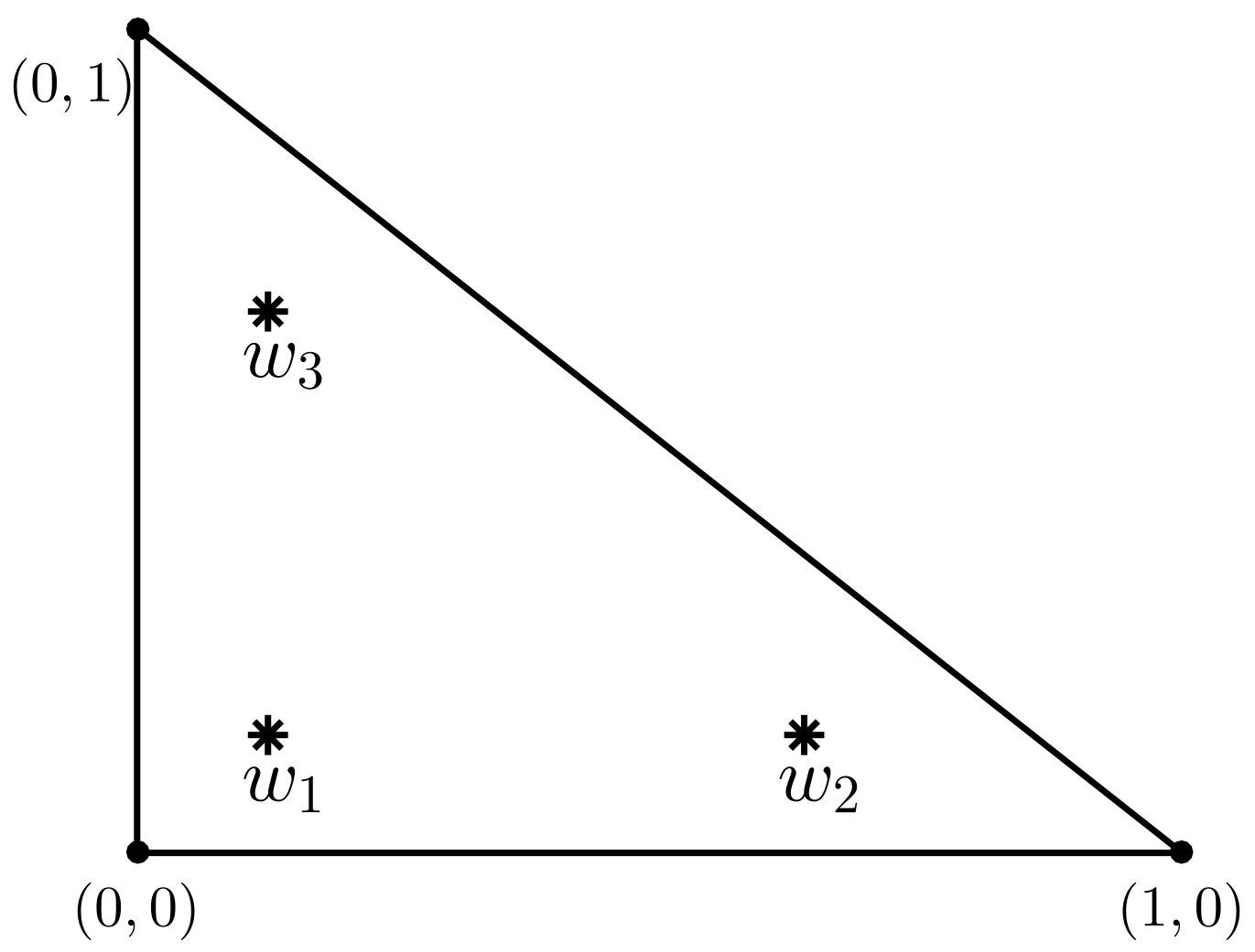
We start with interpolation on the unit simplex

$$\sigma =\left\{\right(s,t\left)\right|0\le s,t,\rho \le 1\},\rho =1-s-t,$$

where $(s,t,\rho )$ are the barycentric coordinates of a point. Then, using an affine transformation, we can generalize the ideas to any triangle in ${\mathbb{R}}^2$.

We approximate a function $h\in C\left(\sigma \right)$ by linear interpolation (see [6,19]):

$$\begin{array}{ccc}\hfill h(s,t)& \approx & {\displaystyle \sum }_{i=1}^{3}h\left(w_i\right)l_i(s,t),\hfill \end{array}$$

(7)

where the nodes

$$w_1=\left({\displaystyle \frac{1}{6}},{\displaystyle \frac{1}{6}}\right),w_2=\left({\displaystyle \frac{1}{6}},{\displaystyle \frac{2}{3}}\right),w_3=\left({\displaystyle \frac{2}{3}},{\displaystyle \frac{1}{6}}\right)$$

(8)

are symmetrically placed inside $\sigma$ (see Figure 2) and the basis functions are given by

$$l_1(s,t)=2\rho -{\displaystyle \frac{1}{3}},l_2(s,t)=2t-{\displaystyle \frac{1}{3}},l_3(s,t)=2s-{\displaystyle \frac{1}{3}}.$$

(9)

Figure 2. Unit simplex and linear interpolation nodes.

Obviously, the interpolation formula (7) has degree of precision 1. Integrating it over $\sigma$, we obtain the numerical integration formula

$$\begin{array}{ccc}\hfill \underset{\sigma }{{\displaystyle \int }}h(s,t)d\sigma & \approx & {\displaystyle \frac{1}{6}}\left[h\left({\displaystyle \frac{1}{6}},{\displaystyle \frac{1}{6}}\right)+h\left({\displaystyle \frac{1}{6}},{\displaystyle \frac{2}{3}}\right)+h\left({\displaystyle \frac{2}{3}},{\displaystyle \frac{1}{6}}\right)\right],\hfill \end{array}$$

(10)

which has degree of precision 2, higher than expected, when linear interpolants are used. This will be important in the convergence analysis of the collocation method.

Next, we extend these formulas from $\sigma$ to any planar triangle $\Delta$ with vertices $\{{\tau }_1,{\tau }_2,{\tau }_3\}$. We define the affine mapping $m:\sigma \underset{onto}{\overset{1-1}{⟶}}\Delta$ by

$$\begin{array}{ccc}\hfill (x,y)& =& m(s,t)=\rho {\tau }_1+t{\tau }_2+s{\tau }_3.\hfill \end{array}$$

(11)

where

$$z_1=(0,0),z_2=(0,1),z_3=(1,0)$$

are the vertices of $\sigma$. Then m maps a polynomial over $\sigma$ into a polynomial of the same degree over $\Delta$ and its inverse acts the same way. With the use of this affine mapping we can define interpolation over any triangle $\Delta$.

Let $h\in C(\Delta )$. Just as in (7), we approximate it by the interpolation polynomial

$$\begin{array}{ccc}\hfill h(x,y)& =& h\left(m(s,t)\right)\approx {\displaystyle \sum }_{i=1}^{3}h\left(m\left(w_i\right)\right)l_i(s,t),(s,t)\in \sigma .\hfill \end{array}$$

(12)

Integrating, we obtain the approximating formula

$$\begin{array}{ccc}\hfill \underset{\Delta }{{\displaystyle \int }}h(x,y)d\Delta & \approx & {\displaystyle \sum }_{i=1}^{3}h\left(m\left(w_i\right)\right)\underset{\sigma }{{\displaystyle \int }}{l}_i(s,t)J_m(s,t)d\sigma ,\hfill \end{array}$$

(13)

where $J_m$ is the Jacobian of the transformation defined in (11). Again, formula (13) is exact for all polynomials of degree 2.

We now define a collocation method based on the piecewise linear interpolation defined above.

Consider ${\mathcal{T}}_n=\{{\Delta }_1,\dots ,{\Delta }_n\}$, a triangulation of $\mathcal{T}$. For each $k\in \{1,\cdots ,n\}$, denote by $\{{\tau }_{1k},{\tau }_{2k},{\tau }_{3k}\}$ the vertices of ${\Delta }_k$ and, as in (11), define the affine mapping $m_k:\sigma \underset{onto}{\overset{1-1}{⟶}}{\Delta }_k$ by

$$\begin{array}{ccc}\hfill (x,y)& =& m_k(s,t)=\rho {\tau }_{1k}+t{\tau }_{2k}+s{\tau }_{3k}.\hfill \end{array}$$

For any given $h\in C\left({\Delta }_k\right)$, we define $P_{n}h$ by

$$\begin{array}{c}\hfill P_{n}h\left(m_k(s,t)\right)={\displaystyle \sum }_{i=1}^{3}h\left(m_k\left(w_i\right)\right)l_i(s,t),(s,t)\in \sigma ,k=1,\dots ,n.\end{array}$$

(14)

For the approximation

$$\begin{array}{ccc}\hfill h(\left(m_k(s,t)\right)& \approx & P_{n}h\left(m_k(s,t)\right),\hfill \end{array}$$

we know from interpolation theory, that the following error estimate holds:

Theorem 2

([20], p. 165). Let Δ be a planar triangle and consider $h\in C^2(\Delta )$. Then,

$$\begin{array}{ccc}\hfill \left|\right|h-P_{n}h{\left|\right|}_{\infty }& \le & c{\delta }^2\left|\right|D_{\Delta }^{2}h{\left|\right|}_{\infty },\hfill \end{array}$$

where $\delta =\mathrm{diameter}(\Delta )$ and ${\displaystyle D_{\Delta }^{r}h=\underset{0\le i\le r}{max}\underset{(\xi ,\eta )\in \Delta }{max}\left|{\displaystyle \frac{{\partial }^{r}h(\xi ,\eta )}{\partial {\xi }^i\partial {\eta }^{r-i}}}\right|}$. The constant c is independent of both h and Δ.

From the interpolation formula (14) we obtain, by integration, the quadrature formula

$$\begin{array}{ccc}\hfill \underset{\mathcal{T}}{{\displaystyle \int }}h\left(w\right)dw& =& {\displaystyle \sum }_{k=1}^n\underset{{\Delta }_k}{{\displaystyle \int }}h\left(w\right)dw\hfill \\ & \approx & {\displaystyle \sum }_{k=1}^n{\displaystyle \sum }_{j=1}^{3}h\left(w_{k,j}\right)\underset{\sigma }{{\displaystyle \int }}{l}_j(s,t)J_{m_k}(s,t)d\sigma ,\hfill \end{array}$$

where $w_{k,j}=m_k\left(w_j\right),k=1,\dots ,n,j=1,\cdots ,3,$ with $w_1,\cdots ,w_3$ given in (8) and $l_j(s,t)$, $j=1,\cdots ,3$ defined in (9).

For the integral Equation (3), we want solutions of the form

$$\begin{array}{ccc}\hfill v_n\left(w\right)& =& {\displaystyle \sum }_{j=1}^3{v}_n\left(w_{k,j}\right)l_j(s,t),\hfill \end{array}$$

for $w=m_k(s,t)\in {\Delta }_k$. We choose the collocation nodes to coincide with the interpolation nodes and find the values $v_n\left(w_{k,j}\right)$ so that Equation (3) is true at the collocation nodes. We obtain the nonlinear system

$$v_n\left(w_i\right)=g\left(w_i,{\displaystyle \sum }_{k=1}^n{\displaystyle \sum }_{j=1}^3{v}_n\left(w_{k,j}\right)\underset{\sigma }{{\displaystyle \int }}k(w_i,m_k(s,t))l_j(s,t)J_{m_k}(s,t)d\sigma +f\left(w_i\right)\right),$$

(15)

for all $i=1,\cdots ,3n$. Once the unknowns $v_n\left(w_i\right)$ are determined, we find the approximate solutions of u and v by

$$\left\{\begin{array}{ccc}{v}_n\left(w\right)\hfill & =& {\displaystyle {\displaystyle \sum }_{i=1}^3{v}_n\left(w_i\right)l_i(s,t),}\hfill \\ u_n\left(w\right)\hfill & =& {\displaystyle {\displaystyle \sum }_{i=1}^3{v}_n\left(w_i\right)\underset{\sigma }{{\displaystyle \int }}k(w,m_k(s,t))l_i(s,t)J_{m_k}(s,t)d\sigma +f\left(w\right),}\hfill \end{array}\right.$$

(16)

for each $w=m_k(s,t)\in {\Delta }_k$.

3.2. Convergence and Error Analysis

To analyze the convergence of the collocation method, denote by $\mathcal{K}$ the operator

$$\begin{array}{ccc}\hfill \mathcal{K}\left(v\right)\left(w\right)& =& g\left(w,\underset{\mathcal{T}}{{\displaystyle \int }}k(w,q)v\left(q\right)dq+f\left(w\right)\right).\hfill \end{array}$$

Then, Equation (3) can be rewritten in operator form as

$$\begin{array}{ccc}\hfill (I-\mathcal{K})v& =& 0,\hfill \end{array}$$

while the collocation Equation (15) is now

$$\begin{array}{ccc}\hfill (I-\mathcal{K}{P}_n)v_n& =& 0.\hfill \end{array}$$

By simple computation, we obtain

$$\begin{array}{ccc}\hfill (I-\mathcal{K}{P}_n)(v-v_n)& =& \mathcal{K}v-\mathcal{K}{P}_{n}v.\hfill \end{array}$$

(17)

The following result follows from standard projection theory, using Theorem 2 and relation (17) (see e.g., [20], Section 3.1).

Theorem 3.

Under the assumptions (H1)–(H4), for all sufficiently large n, the operators $I-\mathcal{K}{P}_n$ are invertible on $C\left(\mathcal{T}\right)$ and have uniformly bounded inverses. Moreover, if $v^{*}$ is the true solution of (3) and $v_n$ is the approximate solution from (15), we have

$$\left|\right|v^{*}-v_n\left|\right|\le c\left|\left|{(I-\mathcal{K}{P}_n)}^{-1}\right|\right|·\left|\right|v^{*}-P_n{v}^{*}\left|\right|,$$

for all sufficiently large n and

$$\left|\right|v^{*}-v_n\left|\right|\le O\left({\delta }^2\right),$$

with ${\displaystyle \delta ={\delta }_n=\underset{1\le k\le n}{max}\mathrm{diameter}\left({\Delta }_k\right),}$ the grid size of the triangulation ${\mathcal{T}}_n$.

Thus, the method is convergent with a rate of convergence of $O\left({\delta }^2\right)$, in general.

However, at the collocation nodes, the method is superconvergent, converging faster than throughout the entire domain. This is our main result.

Theorem 4.

(a) 

Let Δ be a planar triangle and consider functions $h\in C^3(\Delta )$, $\phi \in C(\Delta )$. Then

$$\begin{array}{ccc}\hfill \left|\underset{\Delta }{{\displaystyle \int }}\phi \left(q\right)(I-P_n)h\left(q\right)dq\right|& \le & c{\delta }^3,\hfill \end{array}$$

(18)

where $\delta =\mathrm{diameter}(\Delta )$.

(b) 

Assume the hypotheses of Theorem 3 hold and that $k\in C(\mathcal{T}\times \mathcal{T})$, $v^{*}\in C^3\left(\mathcal{T}\right)$. Then

$$\underset{i=\overline{1,3n}}{max}|v^{*}\left(w_i\right)-v_n\left(w_i\right)|,\underset{i=\overline{1,3n}}{max}|u^{*}\left(w_i\right)-u_n\left(w_i\right)|\le O\left({\delta }^3\right).$$

(19)

Proof. 

(a)

In what follows, c denotes a generic constant.

Since $h\in C^3(\Delta )$, there exist Taylor polynomials $T_1$ and $T_2$ of degree 1 and 2, respectively, of the function h (about some suitable point in $\Delta$), such that

$$\begin{array}{ccc}\hfill \left|\right|h-T_j\left|\right|& \le & c{\delta }^{j+1},j=1,2\hfill \end{array}$$

(20)

and

$$\begin{array}{ccc}\hfill \left|\right|T_2-T_1\left|\right|& \le & c{\delta }^2,\hfill \end{array}$$

(21)

where the constants depend on the derivatives of h.

In addition, since $\phi \in C(\Delta )$, we can find a constant ${\phi }_0$ satisfying

$$\begin{array}{ccc}\hfill \left|\right|\phi -{\phi }_0\left|\right|& \le & c\delta .\hfill \end{array}$$

(22)

Recall that the interpolation formula (7) (and, hence, (12)) is exact for all polynomials of degree 1, which means $(I-P_n)T_1\left(q\right)=0$, for every $q\in \Delta$. So, we can write

$$\begin{array}{ccc}\hfill \phi \left(q\right)(I-P_n)h\left(q\right)& =& \phi \left(q\right)(I-P_n)\left(h\left(q\right)-T_2\left(q\right)\right)\hfill \\ & +& \left(\phi \left(q\right)-{\phi }_0\right)(I-P_n)\left(T_2\left(q\right)-T_1\left(q\right)\right)\hfill \\ & +& {\phi }_0(I-P_n)T_2\left(q\right).\hfill \end{array}$$

Integrating over $\Delta$, we obtain

$$\begin{array}{ccc}\hfill \underset{\Delta }{{\displaystyle \int }}\phi \left(q\right)(I-P_n)h\left(q\right)dq& =& \underset{\Delta }{{\displaystyle \int }}\phi \left(q\right)(I-P_n)\left(h\left(q\right)-T_2\left(q\right)\right)dq\hfill \\ & +& \underset{\Delta }{{\displaystyle \int }}\left(\phi \left(q\right)-{\phi }_0\right)(I-P_n)\left(T_2\left(q\right)-T_1\left(q\right)\right)dq,\hfill \end{array}$$

because

$$\begin{array}{ccc}\hfill \underset{\Delta }{{\displaystyle \int }}{\phi }_0(I-P_n)T_2\left(q\right)dq& =& {\phi }_0\underset{\Delta }{{\displaystyle \int }}(I-P_n)T_2\left(q\right)dq=0,\hfill \end{array}$$

since the numerical integration formula (13) has degree of precision 2. We bound the errors using (20)–(22), to obtain (18).

(b)

By relation (17), at the collocation nodes we have.

$$\begin{array}{ccc}\hfill \underset{i=\overline{1,3n}}{max}|v^{*}\left(w_i\right)-v_n\left(w_i\right)|& \le & \underset{i=\overline{1,3n}}{max}|\mathcal{K}{v}^{*}-\mathcal{K}{P}_n{v}^{*}\left)\left(w_i\right)\right|,\hfill \end{array}$$

so we will find bounds for $|(\mathcal{K}{v}^{*}-\mathcal{K}{P}_n{v}^{*})\left(w_i\right)|$. For each $i=1,\cdots ,3n$, we have

$$\begin{array}{ccc}\hfill |(\mathcal{K}{v}^{*}-\mathcal{K}{P}_n{v}^{*})\left(w_i\right)|& =& \left|g\left(w_i,\underset{\mathcal{T}}{{\displaystyle \int }}k(w_i,q)v^{*}\left(q\right)dq+f\left(w_i\right)\right)\right.\hfill \\ & -& \left.g\left(w_i,\underset{\mathcal{T}}{{\displaystyle \int }}k(w_i,q)P_n{v}^{*}\left(q\right)dq+f\left(w_i\right)\right)\right|\hfill \\ & \le & c\left|{\displaystyle \sum }_{k=1}^n\underset{{\Delta }_k}{{\displaystyle \int }}k(w_i,q)(I-P_n)v^{*}\left(q\right)dq\right|\hfill \\ & \le & c{\displaystyle \sum }_{k=1}^n\left|\underset{{\Delta }_k}{{\displaystyle \int }}k(w_i,q)(I-P_n)v^{*}\left(q\right)dq\right|.\hfill \end{array}$$

On each triangle ${\Delta }_k$, we use part a) for $h\left(q\right)=v^{*}\left(q\right)$ and $\phi \left(q\right)=k(w_i,q)$. Then, we obtain

$$\begin{array}{ccc}\hfill |(\mathcal{K}{v}^{*}-\mathcal{K}{P}_n{v}^{*})\left(w_i\right)|& \le & c{\delta }^3{\displaystyle \sum }_{k=1}^n\underset{{\Delta }_k}{{\displaystyle \int }}dq.\hfill \end{array}$$

Since there are $n=O\left({\delta }^{-2}\right)$ triangles and for each triangle $\mathrm{Area}\left({\Delta }_k\right)=O\left({\delta }^2\right)$, we have a composite error of

$$\begin{array}{ccc}\hfill |(\mathcal{K}{v}^{*}-\mathcal{K}{P}_n{v}^{*})\left(w_i\right)|& \le & O\left({\delta }^3\right).\hfill \end{array}$$

Thus, by Theorem 1, we have (19). □

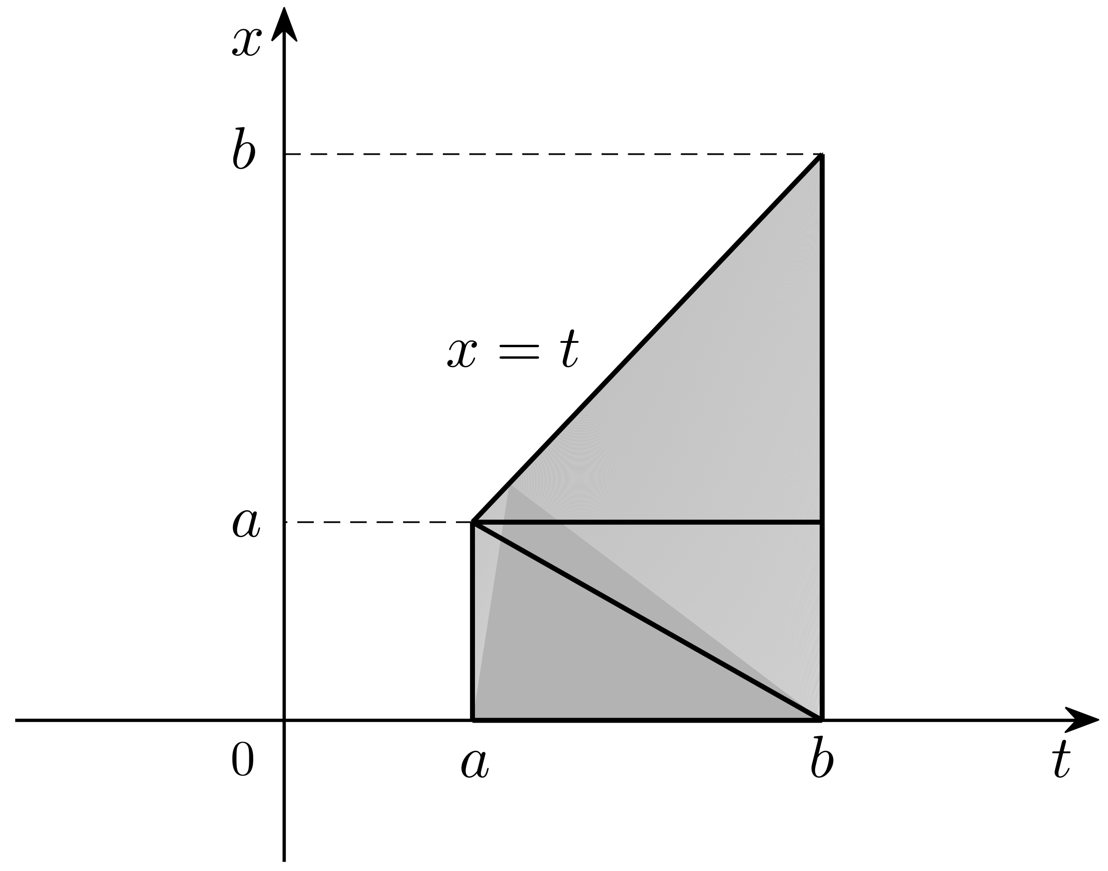
Remark 1.

Let us note that, sometimes, in applications, we encounter MVFHIE’s of the form

$$\begin{array}{ccc}\hfill u(t,x)& =& \underset{0}{\overset{t}{{\displaystyle \int }}}\underset{a}{\overset{b}{{\displaystyle \int }}}k\left(t,x,\xi ,\eta \right)g\left(\xi ,\eta ,u(\xi ,\eta )\right)d\xi d\eta +f(t,x),\hfill \end{array}$$

(23)

where the lower limits of the integrals do not coincide. Such equations come up particularly as integral reformulations of boundary or initial value problems for partial differential equations. In this case, we consider the region of integration

$$\begin{array}{c}\hfill R=\{(t,x)\in {\mathbb{R}}^2|a\le t\le b,0\le x\le t\}\end{array}$$

and start with three triangles that cover it, as seen in Figure 3. From here on, everything works the same as described above for the region $\mathcal{T}$.

Figure 3. Region R of integration for Equation (23).

4. Numerical Experiments

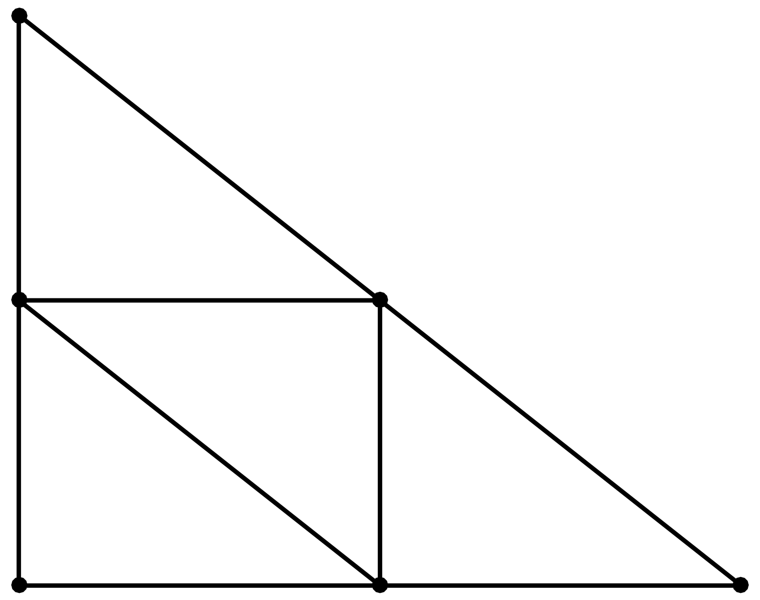
We apply the collocation method described above to several numerical examples. First, let us discuss the triangulation of $\mathcal{T}$ and the way it is refined at each step. Let ${\mathcal{T}}_n=\{{\Delta }_1,\dots ,{\Delta }_n\}$ be a triangulation of $\mathcal{T}$ with mesh size

$${\delta }_n=\underset{1\le k\le n}{max}\mathrm{diameter}\left({\Delta }_k\right).$$

At every iteration, every triangle $\Delta \in {\mathcal{T}}_n$ will be refined into smaller triangles by connecting the midpoints of the three sides of $\Delta$ (see Figure 4). This way, the new triangulations ${\mathcal{T}}_{4n}$ will have four times as many triangles as ${\mathcal{T}}_n$ and grid size

$${\delta }_{4n}={\displaystyle \frac{1}{2}}{\delta }_n.$$

For such triangulations, if the approximation formula has degree of precision r and $e_n\left(h\right)$ denotes the error, then

$$\begin{array}{ccc}\hfill {\displaystyle \frac{e_n\left(h\right)}{e_{4n}\left(h\right)}}& \approx & 2^{r+1}.\hfill \end{array}$$

Figure 4. Refinement of the triangulation.

We use this to assess the rate of convergence in our examples.

For each example, we look at the errors at the collocation points

$$\begin{array}{ccc}\hfill {\epsilon }_n\left(v\right)& =& \underset{i=\overline{1,3n}}{max}|v^{*}\left(w_i\right)-v_n\left(w_i\right)|,\hfill \\ \hfill {\epsilon }_n\left(u\right)& =& \underset{i=\overline{1,3n}}{max}|u^{*}\left(w_i\right)-u_n\left(w_i\right)|,\hfill \end{array}$$

as well as at the values of the ratios

$$r_v={log}_2{\displaystyle \frac{{\epsilon }_n\left(v\right)}{{\epsilon }_{4n}\left(v\right)}},r_u={log}_2{\displaystyle \frac{{\epsilon }_n\left(u\right)}{{\epsilon }_{4n}\left(u\right)}}.$$

Example 1.

Consider the nonlinear integral equation

$$\begin{array}{ccc}\hfill u(x,y)& =& \underset{0}{\overset{x}{\int }}\left(\underset{0}{\overset{1}{\int }}{\displaystyle \frac{\eta }{1+3{\xi }^2}}{\left(u(\xi ,\eta )\right)}^{2}d\xi \right)d\eta +2x^2+1,(x,y)\in \mathcal{T},\hfill \end{array}$$

(24)

where $\mathcal{T}=\{(x,y)\in {\mathbb{R}}^2|0\le x\le 1,0\le y\le x\}$. The exact solution of this equation is $u^{*}(x,y)=1+3x^2.$

We take

$$\begin{array}{ccc}\hfill k(w,q)& =& k\left(x,y,\xi ,\eta \right)={\displaystyle \frac{\eta }{1+3{\xi }^2}},\hfill \\ \hfill g(q,u(q\left)\right)& =& g\left(\eta ,\xi ,u(\eta ,\xi )\right)={\left(u(\eta ,\xi )\right)}^2,\hfill \\ \hfill f\left(w\right)& =& f(x,y)=2x^2+1.\hfill \end{array}$$

We start with $n=1$ triangle, $\mathcal{T}$ itself. The errors in v and u are given in Table 1. Notice that $r_v$ and $r_u$ both converge to the value 3, consistent with the conclusions of Theorem 4. In addition, the table contains the CPU times (in seconds) for each iteration.

Table 1. Errors for Example 1.

n	${\mathit{\epsilon }}_{\mathit{n}}\left(\mathit{v}\right)$	${\mathit{r}}_{\mathit{v}}$	${\mathit{\epsilon }}_{\mathit{n}}\left(\mathit{u}\right)$	${\mathit{r}}_{\mathit{u}}$	CPU Time
1	3.563 $\times {10}^{-2}$		1.350 $\times {10}^{-2}$		0.31
4	9.747 $\times {10}^{-3}$	1.87	3.422 $\times {10}^{-3}$	1.98	0.76
16	1.459 $\times {10}^{-3}$	2.74	4.521 $\times {10}^{-4}$	2.92	2.69
64	1.862 $\times {10}^{-4}$	2.97	5.459 $\times {10}^{-5}$	3.05	13.45

Example 2.

Next, we consider the integral equation [17]

$$\begin{array}{ccc}\hfill u(x,y)& =& 16\underset{0}{\overset{x}{\int }}\left(\underset{0}{\overset{1}{\int }}{e}^{x+y+\xi +\eta }{\left(u(\xi ,\eta )\right)}^{3}d\eta \right)d\xi +f(x,y),(x,y)\in \mathcal{T},\hfill \end{array}$$

(25)

where $f(x,y)=e^{5x+y}+e^{x+y+4}-e^{5x+y+4}$ and $\mathcal{T}=\{(x,y)\in {\mathbb{R}}^2|0\le x\le 1,0\le y\le x\}$. The true solution of Equation (25) is $u^{*}(x,y)=e^{x+y}.$

In this example, we take

$$\begin{array}{ccc}\hfill k(w,q)& =& k\left(x,y,\xi ,\eta \right)=e^{x+y},\hfill \\ \hfill g(q,u(q\left)\right)& =& g\left(\eta ,\xi ,u(\eta ,\xi )\right)=e^{\xi +\eta }{\left(u(\eta ,\xi )\right)}^3,\hfill \end{array}$$

and the function $f(x,y)$ given above. Again we start with one triangle, $\mathcal{T}$. The numerical approximations, the errors and the CPU times are given in Table 2. Again, they are in good agreement with the theoretical results of Theorem 4. In addition, one can notice that the accuracy of the present method is higher than the one in [17], where collocation at Gauss–Bernoulli nodes was used.

Table 2. Errors for Example 2.

n	${\mathit{\epsilon }}_{\mathit{n}}\left(\mathit{v}\right)$	${\mathit{r}}_{\mathit{v}}$	${\mathit{\epsilon }}_{\mathit{n}}\left(\mathit{u}\right)$	${\mathit{r}}_{\mathit{u}}$	CPU Time
1	$3.938\times {10}^{-2}$		$1.862\times {10}^{-2}$		0.33
4	$1.092\times {10}^{-2}$	1.85	$4.753\times {10}^{-3}$	1.97	0.75
16	$1.669\times {10}^{-3}$	2.71	$6.323\times {10}^{-4}$	2.91	3.01
64	$2.146\times {10}^{-4}$	2.96	$7.796\times {10}^{-5}$	3.02	14.27

Example 3.

As an example of the type (23), described in Remark 1, consider the equation

$$\begin{array}{ccc}\hfill u(t,x)& =& {\displaystyle \frac{2}{3}}\underset{0}{\overset{t}{\int }}\left(\underset{1}{\overset{2}{\int }}{e}^{x-\eta }u(\xi ,\eta )d\xi \right)d\eta ,(x,t)\in R,\hfill \end{array}$$

(26)

where the domain of integration is $R=\{(t,x)\in {\mathbb{R}}^2|1\le t\le 2,0\le x\le t\}$ and whose exact solution is $u^{*}(t,x)=t{e}^x.$

Here, we consider

$$\begin{array}{ccc}\hfill k(w,q)& =& k\left(t,x,\xi ,\eta \right)={\displaystyle \frac{2}{3}}{e}^x,\hfill \\ \hfill g(q,u(q\left)\right)& =& g\left(\xi ,\eta ,u(\xi ,\eta )\right)=e^{-\eta }u(\xi ,\eta ),\hfill \\ \hfill f\left(w\right)& \equiv & 0.\hfill \end{array}$$

Now we start with three triangles covering R, as in Figure 3. The results are displayed in Table 3 and again, they confirm the theoretical findings of Theorem 4.

Table 3. Errors for Example 2.

n	${\mathit{\epsilon }}_{\mathit{n}}\left(\mathit{v}\right)$	${\mathit{r}}_{\mathit{v}}$	${\mathit{\epsilon }}_{\mathit{n}}\left(\mathit{u}\right)$	${\mathit{r}}_{\mathit{u}}$	CPU Time
3	$1.975\times {10}^{-2}$		$1.002\times {10}^{-2}$		0.47
12	$5.219\times {10}^{-3}$	1.92	$2.289\times {10}^{-3}$	2.13	2.90
48	$7.041\times {10}^{-4}$	2.89	$2.881\times {10}^{-4}$	2.99	9.31

Remark 2.

The method was implemented in Matlab 2016. The integrals in System (15) were evaluated with the integral2 function, which uses tiled adaptive quadratures. The system was solved with the fsolve function, using large-scale (trust-region, trust-region-dogleg, and Levenberg–Marquardt) optimization algorithms.

5. Conclusions and Future Work Ideas

We studied a collocation method for approximating the solutions of two-dimensional MVFHIE’s. As in [18], the collocation method is applied to a reformulation of the equation in a new unknown. This makes for a more efficient method from the implementation point of view, reducing the computational cost, as the integrals needed in the coefficients of the resulting system only have to be evaluated once per iteration. The collocation method described here is based on a special type of linear interpolation on triangles, which leads to a superconvergent method at the collocation nodes. Another aspect worth pointing out is the fact that since our collocation method is based on interpolation, a rigorous convergence analysis is easier than for methods based directly on quadratures. Compared to other interpolation-based collocation methods, since the degree of precision of the numerical integration formula is higher, this method converges faster, without having to increase the degree of the interpolants, which, in turn, would increase the size of the nonlinear system of the coefficients. It can be seen from the numerical examples that the CPU times are relatively small, but the precision of the approximate solution is quite good. These are the major advantages of this numerical method.

The choice of interpolation nodes was important. They were chosen so that the corresponding quadrature formula has a higher precision than expected with linear interpolants. In addition, the fact that they are symmetrical simplifies the implementation of the method. Last but not least, as the interpolation/collocation nodes are all interior to the triangles, such methods could work well for some singular kernels, especially if the singularities occur on the boundary of the domain. For instance, integral reformulations of the heat equation with initial or boundary values would lead to such integral equations.

Further, more complicated regions of integration can be considered, with the upper limit of integration some function $\phi :[a,b]\to [a,b]$,

$$\begin{array}{ccc}\hfill u(x,y)& =& \underset{a}{\overset{\phi \left(x\right)}{{\displaystyle \int }}}\underset{a}{\overset{b}{{\displaystyle \int }}}k\left(x,y,\xi ,\eta \right)g\left(\xi ,\eta ,u(\xi ,\eta )\right)d\xi d\eta +f(x,y).\hfill \end{array}$$

Such equations could be handled the same way, if $\phi$ is smooth enough and a suitable triangulation can be considered on the curved boundary.

The case of an infinite domain could also be studied, to see if an adapted collocation method of this type would work, with convenient triangulations and, perhaps, some extra theoretical assumptions on the kernel.

Last but not least, other interpolation/collocation nodes on triangles can be considered.