A Super-Twisting Extended State Observer for Nonlinear Systems

Abstract

Disturbances and uncertainties are the main concerns in control systems. To obtain this information in real time, the extended state observer is proposed as the core of the active disturbance rejection control. However, the estimation errors of extended state observer cannot converge to zero in the presents of unknown but bounded disturbances, which will bring unexpected tracking errors to the closed-loop system. By taking advantage of the linear extended state observer and the super-twisting algorithm, the super-twisting extended state observer is proposed to deal with the non-diminishing second-order derivable disturbances in this paper. The asymptotic convergence of the super-twisting extended state observer and the controller are proved by the Lyapunov method. Moreover, the effectiveness and robustness of the super-twisting extended state observer are verified by simulation analysis. Simulation results show that the proposed super-twisting extended state observer maintains the minimized estimation error with less settling time compared the with linear extended state observer. The tracking performance of the controller with the proposed observer is greatly improved.

1. Introduction

Disturbances and uncertainties exist widely in practical systems, which may affect the tracking performance badly or even the system stability [1,2]. Thus, disturbance rejection becomes a key part of the system controller design process. It is well known that the measurable disturbance can be attenuated by feedforward. However, disturbances in many systems are often unmeasurable or cannot be accurately measured. An effective approach to this problem is to estimate and then compensate for the disturbance in real time. On this basis, the uncertainty can also be classified as a part of the disturbance, and the disturbance observer technique is generated [3]. As the core of active disturbance rejection control (ADRC) proposed by Han [4], the extended state observer (ESO) can treat unmodeled dynamics, uncertainties and external disturbances as a generalized disturbance or total disturbance. In order to simplify the parameter adjustment, the ESO is simplified to linear ESO (LESO) by utilizing the linear function instead of the nonlinear function [5], which greatly promotes its theoretical research [6,7,8,9,10] and applications [11,12,13]. For the convergence of ESO, some scholars have carried out relevant studies. In the case that assuming the system dynamics and its derivatives are bounded, YOO [14] analyzed the performance and convergence of LESO for state estimation, and further analyzed and proved the convergence of discrete ESO [15]. Yang [16] weakened the assumptions and proved that the LESO estimation error is bounded under the condition that the system dynamics or their derivative are bounded. Zheng [17] analyzed the stability of LADRC (linear active disturbance rejection control) for nonlinear time-varying systems with uncertainties. When the dynamics of the system model are fully known, the system is asymptotically stable. However, when there exists model uncertainty, both the ESO estimation error and controller tracking error have upper bounds and decrease monotonically with increasing bandwidth. Instead of using the Lyapunov method, Zheng analyzed the stability of ESO and ADRC by solving the differential equation, and the relationship between error boundary and ADRC bandwidth was further studied [18]. In addition, some references pointed out that the differential of the total disturbance is the only assumption that needs to be made, and it is usually assumed that the derivative of the total disturbance is bounded or satisfies the local Lipschitz condition [19,20,21]. However, the estimation error of LESO cannot be eliminated to zero in the presence of unknown, derivable but bounded disturbances, which will lead to unexpected tracking errors of the closed-loop system. Thus, it is of significance to explore the performance improvements of LESO and perform the analysis.

Sliding mode control (SMC) can effectively deal with the uncertainty of the system, and higher-order SMC is generated to attenuate chattering phenomenon and improve tracking performance [22]. As a well-known second-order SMC control method, the super-twisting algorithm [23] can effectively eliminate the chattering with excellent convergence performance and has been widely used to design controllers [24,25,26] and observers [27,28,29]. Therefore, the second order sliding mode technique is introduced into the design of the LESO to ensure that the estimation errors can converge to zero in this paper.

Motivated by SMC and ADRC, this paper proposes a novel disturbance observer based on the super-twisting algorithm, namely the super-twisting extended state observer (STESO). The main contributions are the following: (1) A novel asymptotically convergent extended state observer is proposed by utilizing the super-twisting algorithm. Compared with conventional extended state observers, the proposed STESO can improve the observation ability and drive the estimation error to zero asymptotically. (2) A strict Lyapunov analysis is carried out for STESO and the related closed-loop system. The STESO based controller is asymptotically stable and can maintain zero tracking error.

The remaining parts of this paper are organized as follows. In Section 2, the problem formulation is described. Section 3 gives the main results and theoretical analysis. Section 4 carries out some numerical simulations with disturbance and results analysis. The conclusions are given in Section 5.

2. Problem Formulation

As introduced in preliminaries, if the nonlinear system is written as

$$\begin{array}{c}\hfill \left\{\begin{array}{c}{\dot{x}}_1=x_2\hfill \\ {\dot{x}}_2=x_3\hfill \\ \cdots \hfill \\ {\dot{x}}_n=bu+f\hfill \end{array}\right.,\end{array}$$

(1)

where $x_i\left(i=1,2,\cdots ,n\right)$ are states of the nonlinear system, u is the input, b represents the input gain, and f denotes the differentiable total disturbance, then, according to the principle of the ADRC algorithm, an extended state $x_{n+1}=f$ is designed and Equation (1) can be written as

$$\begin{array}{c}\hfill \left\{\begin{array}{c}{\dot{x}}_1=x_2\hfill \\ {\dot{x}}_2=x_3\hfill \\ \cdots \hfill \\ {\dot{x}}_n=x_{n+1}+bu\hfill \\ {\dot{x}}_{n+1}=h\hfill \end{array}\right.,\end{array}$$

(2)

where $h=\dot{f}$ is the derivative of f and it is assumed that

$$\begin{array}{c}\hfill \left|h\right|\le L_h.\end{array}$$

(3)

The LESO of Equation (2) can be designed as

$$\begin{array}{c}\hfill \left\{\begin{array}{c}{\dot{z}}_1=z_2+{\beta }_1{e}_1\hfill \\ {\dot{z}}_2=z_3+{\beta }_2{e}_1\hfill \\ \cdots \hfill \\ {\dot{z}}_n=z_{n+1}+{\beta }_n{e}_1+bu\hfill \\ {\dot{z}}_{n+1}={\beta }_{n+1}{e}_1\hfill \end{array}\right.,\end{array}$$

(4)

where $e_i=x_i-z_i$, and ${\beta }_i\left(i=1,2,\cdots ,n+1\right)$ are the error feedback gains. Subtracting Equation (4) from Equation (2), the estimation error can be formulated as

$$\begin{array}{c}\hfill \left\{\begin{array}{c}{\dot{e}}_1=e_2-{\beta }_1{e}_1\hfill \\ {\dot{e}}_2=e_3-{\beta }_2{e}_1\hfill \\ \cdots \hfill \\ {\dot{e}}_n=e_{n+1}-{\beta }_n{e}_1\hfill \\ {\dot{e}}_{n+1}=h-{\beta }_{n+1}{e}_1\hfill \end{array}\right.,\end{array}$$

(5)

which can be simplified as

$$\dot{e}=Ae+B_{h}h,$$

(6)

where $e={\left[\begin{array}{cccc}{e}_1& e_2& \cdots & e_{n+1}\end{array}\right]}^T$ and

$$\begin{array}{c}\hfill A=\left[\begin{array}{cccc}-{\beta }_1& 1& ⋮& 0\\ -{\beta }_2& 0& ⋮& 0\\ \cdots & \cdots & \ddots & \cdots \\ -{\beta }_{n+1}& 0& ⋮& 0\end{array}\right],B_h={\left[0,0,\cdots ,0,1\right]}^T.\end{array}$$

(7)

In Equation (7), ${\beta }_i\left(i=1,2,\cdots ,n+1\right)$ are tuned to make A Hurwitz. Then, there exist unique positive definite matrices $P_1$ and $Q_1$ such that

$$\begin{array}{c}\hfill A^T{P}_1+P_{1}A=-Q_1.\end{array}$$

Therefore, a Lyapunov candidate function can be designed as $V\left(e\right)=e^T{P}_{1}e$. Differentiating $V\left(e\right)$ obtains

$$\begin{array}{cc}\hfill \dot{V}\left(e\right)& =-e^T{Q}_{1}e+2e^T{P}_1{B}_{h}h\hfill \\ \hfill & \le -{\lambda }_{min}\left(Q\right){∥e∥}_2^2+2{∥e∥}_2∥P_1{B}_h∥L_h\hfill \\ \hfill & \le -\left({\lambda }_{min}\left(Q\right){∥e∥}_2-2∥P_1{B}_h∥L_h\right){∥e∥}_2,\hfill \end{array}$$

(8)

which indicates that $\dot{V}\left(e\right)\le 0$ for any

$$\begin{array}{c}\hfill {∥e∥}_2\ge \frac{2∥P_1{B}_h∥L_h}{{\lambda }_{min}\left(Q\right)}.\end{array}$$

(9)

It can be seen from Equation (9) that the estimation error of the LESO (4) is bounded under condition (3). However, the bounded estimation error will limit the implementation of many control methods.

3. Main Results

The main concern of this paper is to maintain the zero-estimation error of the extended state observer and achieve the accurate estimation of the total disturbance. To this end, the STESO is proposed based on the super-twisting sliding mode control algorithm.

3.1. Stability Analysis of STESO

Firstly, the sliding manifold is designed as

$$\begin{array}{c}\hfill \sigma =c_1{e}_1+c_2{e}_2+\cdots +c_{n-1}{e}_{n-1}+e_n,\end{array}$$

(10)

where $c_i\left(i=1,2,\cdots ,n-1\right)$ are positive constants. To avoid the residual estimation errors by the LESO, the STESO is designed as

$$\begin{array}{c}\hfill \left\{\begin{array}{c}{\dot{z}}_1=z_2+{\beta }_1{e}_1\hfill \\ {\dot{z}}_2=z_3+{\beta }_2{e}_1\hfill \\ \cdots \hfill \\ {\dot{z}}_n=z_{n+1}+u_a+bu\hfill \\ {\dot{z}}_{n+1}=k_3\mathrm{sgn}\left(\sigma \right)+k_4\sigma \hfill \end{array}\right.,\end{array}$$

(11)

where $u_a$ is an auxiliary error feedback which is applied to handle the bounded total disturbance, and and $k_3$ and $k_4$ are parameters to be tuned. Specifically, $k_4\sigma$ is elaborately designed to ensure the asymptotic convergence of STESO. Substituting Equation (11) from (2), the estimation error of STESO can be written as

$$\begin{array}{c}\hfill \left\{\begin{array}{c}{\dot{e}}_1=e_2-{\beta }_1{e}_1\hfill \\ {\dot{e}}_2=e_3-{\beta }_2{e}_1\hfill \\ \cdots \hfill \\ {\dot{e}}_n=e_{n+1}-u_a\hfill \\ {\dot{e}}_{n+1}=h-k_3\mathrm{sgn}\left(\sigma \right)-k_4\sigma \hfill \end{array}\right..\end{array}$$

(12)

As h is unknown but bounded, we take the advantage of SMC to eliminate the estimation error to zero. In this paper, the super-twisting algorithm is utilized to design $u_a$. By differentiating Equation (10), one obtains

$$\begin{array}{cc}\hfill \dot{\sigma }& =c_1{\dot{e}}_1+c_2{\dot{e}}_2+\cdots +c_{n-1}{\dot{e}}_{n-1}+{\dot{e}}_n\hfill \\ \hfill & =c_1{e}_2+c_2{e}_3+\cdots c_{n-1}{e}_n-\hfill \\ \hfill & \left(c_1{\beta }_1+c_2{\beta }_2+\cdots +c_{n-1}{\beta }_{n-1}\right)e_1+e_{n+1}-u_a.\hfill \end{array}$$

(13)

According to the super-twisting algorithm, $u_a$ is designed as

$$\begin{array}{cc}\hfill u_a=& c_1{e}_2+c_2{e}_3+\cdots c_{n-1}{e}_n+k_1{\left|\sigma \right|}^{\frac{1}{2}}\mathrm{sgn}\left(\sigma \right)+k_2\sigma -\hfill \\ \hfill & \left(c_1{\beta }_1+c_2{\beta }_2+\cdots +c_{n-1}{\beta }_{n-1}\right)e_1.\hfill \end{array}$$

(14)

Then, the derivative of $\sigma$ can be presented as

$$\begin{array}{c}\hfill \left\{\begin{array}{c}\dot{\sigma }=-k_1{\left|\sigma \right|}^{\frac{1}{2}}\mathrm{sgn}\left(\sigma \right)-k_2\sigma +e_{n+1}\hfill \\ {\dot{e}}_{n+1}=-k_3\mathrm{sgn}\left(\sigma \right)-k_4\sigma +h\hfill \end{array}\right..\end{array}$$

(15)

Lemma 1

([30]). Consider the system in (15), and suppose there exists a Lyapunov function $V\left(\eta \right)$ defined on a neighborhood $U\in {\mathbb{R}}^n$ of the origin, and

$$\begin{array}{c}\hfill \dot{V}\left(\eta \right)\le -{\beta }_1{V}^{{\alpha }_1}\left(\eta \right)\end{array}$$

(16)

with $\left(\eta \right)\in U\setminus \left\{0\right\}$, $0<{\alpha }_1<1$ and ${\beta }_1>0$. Then the system is locally finite time stable, and

$$\begin{array}{c}\hfill T\le \frac{1}{{\beta }_1\left(1-{\alpha }_1\right)}{\left|V\left(\eta \left(0\right)\right)\right|}^{1-{\alpha }_1}\end{array}$$

(17)

is the time needed to reach $V\left(\eta \right)=0$, where $\eta (0)$ is the initial values of η.

Theorem 1.

If Equation (3) holds,

$$\begin{array}{c}\hfill A_e=\left[\begin{array}{cccc}-{\beta }_1& 1& ⋮& 0\\ -{\beta }_2& 0& ⋮& 0\\ \cdots & \cdots & \ddots & \cdots \\ -{\beta }_{n-1}-c_1& -c_2& ⋮& -c_{n-1}\end{array}\right]\end{array}$$

(18)

is Lipchitz. Then the gains $k_i$ can be selected highly enough so that the origin of Equation (15) is an equilibrium point. Therefore, the proposed continuous auxiliary feedback controller (14) guarantees that σ converges to the origin in finite time and the estimation errors converge to zero asymptotically.

Proof. 

In this section, two steps are provided to complete the proof of Theorem 1 for clarity. $e_{n+1}$ is replaced by $z_{\sigma }$.

Step 1. The convergence of the manifold $\sigma$ is proved first. To this end, the Lyapunov candidate function of Equation (15) is designed as

$$\begin{array}{cc}\hfill V_{\sigma }=& 2k_3\left|\sigma \right|+k_4{\sigma }^2+\frac{1}{2}{z}_{\sigma }^2+\hfill \\ \hfill & \frac{1}{2}{\left(k_1{\left|\sigma \right|}^{\frac{1}{2}}\mathrm{sgn}\left(\sigma \right)+k_2\sigma -z_{\sigma }\right)}^2\hfill \\ \hfill =& {\zeta }^T{P}_{\sigma }\zeta \hfill \end{array}$$

(19)

where $\zeta ={\left[\begin{array}{ccc}{\left|\sigma \right|}^{\frac{1}{2}}\mathrm{sgn}\left(\sigma \right)& \sigma & z_{\sigma }\end{array}\right]}^T$ and

$$\begin{array}{c}\hfill P_{\sigma }=\frac{1}{2}\left[\begin{array}{ccc}4k_3+k_1^2& k_1{k}_2& -k_1\\ k_1{k}_2& 2k_4+k_2^2& -k_2\\ -k_1& -k_2& 2\end{array}\right].\end{array}$$

(20)

When $\sigma \ne 0$, the derivative of Equation (19) can be written as

$$\begin{array}{cc}\hfill {\dot{V}}_{\sigma }=& 2k_3\mathrm{sgn}\left(\sigma \right)\dot{\sigma }+2k_4\sigma \dot{\sigma }+z_{\sigma }{\dot{z}}_{\sigma }+2\Delta {\zeta }^{T}P\zeta +\hfill \\ \hfill & \left(k_1{\left|\sigma \right|}^{\frac{1}{2}}\mathrm{sgn}\left(\sigma \right)+k_2\sigma -z_{\sigma }\right)\left(k_1\frac{1}{2{\left|\sigma \right|}^{\frac{1}{2}}}\dot{\sigma }+k_2\dot{\sigma }-{\dot{z}}_{\sigma }\right)\hfill \\ \hfill =& -2k_1{k}_3{\left|\sigma \right|}^{\frac{1}{2}}-2k_2{k}_3\left|\sigma \right|+2k_3{z}_{\sigma }\mathrm{sgn}\left(\sigma \right)-\hfill \\ \hfill & 2k_1{k}_4{\left|\sigma \right|}^{\frac{3}{2}}-2k_2{k}_4{\sigma }^2+2k_4\sigma z_{\sigma }-k_3{z}_{\sigma }\mathrm{sgn}\left(\sigma \right)-\hfill \\ \hfill & k_4{z}_{\sigma }\sigma -k_1\frac{1}{2{\left|\sigma \right|}^{\frac{1}{2}}}{\dot{\sigma }}^2-k_2{\dot{\sigma }}^2+k_1{k}_3{\left|\sigma \right|}^{\frac{1}{2}}+k_1{k}_4{\left|\sigma \right|}^{\frac{3}{2}}+\hfill \\ \hfill & k_2{k}_3\left|\sigma \right|+k_2{k}_4{\sigma }^2-k_3{z}_{\sigma }\mathrm{sgn}\left(\sigma \right)-k_4{z}_{\sigma }\sigma +2\Delta {\zeta }^{T}P\zeta \hfill \\ \hfill =& -\frac{1}{{\left|\sigma \right|}^{\frac{1}{2}}}{\zeta }^T{\Omega }_1\zeta -{\zeta }^T{\Omega }_2\zeta +2\Delta {\zeta }^{T}P\zeta ,\hfill \end{array}$$

(21)

where

$$\begin{array}{cc}\hfill & \Delta {\zeta }^T=\left[\begin{array}{c}0\\ 0\\ h\end{array}\right],{\Omega }_1=\frac{k_1}{2}\left[\begin{array}{ccc}2k_3+k_1^2& 0& -k_1\\ 0& 2k_4+5k_2^2& -3k_2\\ -k_1& -3k_2& 1\end{array}\right],\hfill \\ \hfill & {\Omega }_2=k_2\left[\begin{array}{ccc}{k}_3+2k_1^2& 0& 0\\ 0& k_4+k_2^2& -k_2\\ 0& -k_2& 1\end{array}\right].\hfill \end{array}$$

(22)

To continue the analysis, we define

$$\begin{array}{cc}\hfill V_{\Delta }& =2\Delta {\zeta }^{T}P\zeta \hfill \\ \hfill & =h\left(-k_1{\left|\sigma \right|}^{\frac{1}{2}}\mathrm{sgn}\left(\sigma \right)-k_2\sigma +2z_{\sigma }\right)\hfill \\ \hfill & \le L_h\left(-k_1{\left|\sigma \right|}^{\frac{1}{2}}\mathrm{sgn}\left(\sigma \right)-k_2\sigma +2z_{\sigma }\right)\hfill \\ \hfill & \le \frac{1}{{\left|\sigma \right|}^{\frac{1}{2}}}\left(L_h{k}_1\left|\sigma \right|+2L_h{\left|\sigma \right|}^{\frac{1}{2}}\left|z_{\sigma }\right|\right)+k_2{L}_h\left|\sigma \right|\hfill \\ \hfill & =\frac{1}{{\left|\sigma \right|}^{\frac{1}{2}}}{\xi }^T{\Delta }_1\xi +{\xi }^T{\Delta }_2\xi ,\hfill \end{array}$$

(23)

where $\xi ={\left[\begin{array}{ccc}{\left|\sigma \right|}^{\frac{1}{2}}& \left|\sigma \right|& \left|z_{\sigma }\right|\end{array}\right]}^T$ and

$$\begin{array}{c}\hfill {\Delta }_1=\left[\begin{array}{ccc}{L}_h{k}_1& 0& L_h\\ 0& 0& 0\\ L_h& 0& 0\end{array}\right],{\Delta }_2=\left[\begin{array}{ccc}{k}_2{L}_h& 0& 0\\ 0& 0& 0\\ 0& 0& 0\end{array}\right].\end{array}$$

(24)

If $k_i\left(i=1,2,3,4\right)$ are selected properly such that

$$\begin{array}{c}\hfill {\Omega }_1-{\Delta }_1>0,{\Omega }_2-{\Delta }_2>0\end{array}$$

(25)

hold, one obtains

$$\begin{array}{c}\hfill {\dot{V}}_{\sigma }\le -\frac{1}{{\left|\sigma \right|}^{\frac{1}{2}}}{\xi }^T\left({\Omega }_1-{\Delta }_1\right)\xi -{\xi }^T\left({\Omega }_2-{\Delta }_2\right)\xi \end{array}$$

(26)

according to Equations (21) and (23). The stability of the sliding manifold given by (10) is proven. Furthermore, considering the practice that ${\lambda }_{min}\left(P\right){∥\xi ∥}^2\le V_{\sigma }\le {\lambda }_{max}\left(P\right){∥\xi ∥}^2$ and $\left|\sigma \right|\le {∥\xi ∥}^2$, we obtain

$$\begin{array}{cc}\hfill {\dot{V}}_{\sigma }& \le -\frac{1}{{\left|\sigma \right|}^{\frac{1}{2}}}{\lambda }_{min}\left({\Omega }_1-{\Delta }_1\right){∥\xi ∥}^2-{\lambda }_{min}\left({\Omega }_2-{\Delta }_2\right){∥\xi ∥}^2\hfill \\ \hfill & \le -{\lambda }_{min}\left({\Omega }_1-{\Delta }_1\right)∥\xi ∥-{\lambda }_{min}\left({\Omega }_2-{\Delta }_2\right){∥\xi ∥}^2\hfill \\ \hfill & \le -\frac{{\lambda }_{min}\left({\Omega }_1-{\Delta }_1\right){\lambda }_{max}{\left(P\right)}^{\frac{1}{2}}}{{\lambda }_{max}\left(P\right)}{V}_{\sigma }^{\frac{1}{2}}-\frac{{\lambda }_{min}\left({\Omega }_2-{\Delta }_2\right)}{{\lambda }_{max}\left(P\right)}{V}_{\sigma }\hfill \\ \hfill & \le -\frac{{\lambda }_{min}\left({\Omega }_1-{\Delta }_1\right){\lambda }_{max}{\left(P\right)}^{\frac{1}{2}}}{{\lambda }_{max}\left(P\right)}{V}_{\sigma }^{\frac{1}{2}},\hfill \end{array}$$

(27)

which indicates that the sliding manifold converges to zero in finite time and reaches that value at most after

$$\begin{array}{c}\hfill T\le \frac{2{\lambda }_{max}\left(P\right)}{{\lambda }_{min}\left({\Omega }_1-{\Delta }_1\right){\lambda }_{max}{\left(P\right)}^{\frac{1}{2}}}{V_{\sigma }}^{\frac{1}{2}}\left(0\right)\end{array}$$

(28)

according to Lemma 1. The proposed $u_a$ ensures that the estimation errors are always kept on the manifold $\sigma$. Specifically, $z_{\sigma }$ converges to zero according to Barbalat’s lemma at the same time.

Step 2. It can be inferred from (10) and (12) that

$$\begin{array}{c}\hfill \left\{\begin{array}{c}{\dot{e}}_1=e_2-{\beta }_1{e}_1\hfill \\ {\dot{e}}_2=e_3-{\beta }_2{e}_1\hfill \\ \cdots \hfill \\ {\dot{e}}_{n-1}=-{\beta }_{n-1}{e}_1-c_1{e}_1-c_2{e}_2-\cdots -c_{n-1}{e}_{n-1}\hfill \end{array}\right..\end{array}$$

(29)

To facilitate the description, (29) is written as

$$\begin{array}{c}\hfill {\dot{e}}_e=A_e{e}_e,\end{array}$$

(30)

where $e_e={\left[e_1{e}_2\cdots e_{n-1}\right]}^T$. Since $A_e$ is Lipchitz according to the given condition, it is easy to conclude that (30) is asymptotically stable. This completes the proof. □

3.2. Closed-Loop Stability Analysis of STESO-Based Controller

For system (1), the control input u can be designed as

$$\begin{array}{c}\hfill u=\frac{-{\gamma }_1{z}_1-{\gamma }_2{z}_2-\cdots -{\gamma }_n{z}_n-z_{n+1}}{b},\end{array}$$

(31)

which will drive the states of Equation (1) to its origin. Therefore, the closed-loop system is given by

$$\begin{array}{c}\hfill \left\{\begin{array}{c}{\dot{x}}_1=x_2\hfill \\ {\dot{x}}_2=x_3\hfill \\ \cdots \hfill \\ {\dot{x}}_n=-K_{x}x+K_{e}e\hfill \\ {\dot{e}}_1=e_2-{\beta }_1{e}_1\hfill \\ {\dot{e}}_2=e_3-{\beta }_2{e}_2\hfill \\ \cdots \hfill \\ {\dot{e}}_n=e_{n+1}-u_a\hfill \\ {\dot{e}}_{n+1}=h-k_3\mathrm{sgn}\left(\sigma \right)-k_4\sigma \hfill \end{array}\right.,\end{array}$$

(32)

where $K_x={\left[{\gamma }_1{\gamma }_2\cdots {\gamma }_n\right]}^T$ and $K_e={\left[K_x^{T}1\right]}^T$.

Equation (32) also can be rewritten as

$$\begin{array}{c}\hfill \dot{\epsilon }=\left[\begin{array}{cc}{A}_1& B_e\\ 0& A_2\end{array}\right]\epsilon +B_h\left(h-k_3\mathrm{sgn}\left(\sigma \right)-k_4\sigma \right)-B_u{u}_a,\end{array}$$

(33)

where $\epsilon ={\left[x_1{x}_2\cdots x_n{e}_1{e}_2,\cdots e_{n+1}\right]}^T$

$$\begin{array}{cc}\hfill & A_1={\left[\begin{array}{cccc}0& 1& ⋮& 0\\ 0& 0& ⋮& 0\\ \cdots & \cdots & \ddots & \cdots \\ {\gamma }_1& {\gamma }_2& ⋮& {\gamma }_n\end{array}\right]}_{n\times n},\hfill \\ \hfill & B_e={\left[\begin{array}{cccc}0& 0& ⋮& 0\\ 0& 0& ⋮& 0\\ \cdots & \cdots & \ddots & \cdots \\ {\gamma }_1& {\gamma }_2& ⋮& 1\end{array}\right]}_{n\times \left(n+1\right)},\hfill \\ \hfill & A_2={\left[\begin{array}{cccc}-{\beta }_1& 1& ⋮& 0\\ -{\beta }_2& 0& ⋮& 0\\ \cdots & \cdots & \ddots & \cdots \\ 0& 0& ⋮& 0\end{array}\right]}_{\left(n+1\right)\times \left(n+1\right)},\hfill \\ \hfill & B_h={\left[\begin{array}{cccc}0& 0& \cdots & 1\end{array}\right]}_{1\times \left(2n+1\right)}^T,\hfill \\ \hfill & B_u={\left[\begin{array}{ccccc}0& 0& \cdots & 1& 0\end{array}\right]}_{1\times \left(2n+1\right)}^T.\hfill \end{array}$$

(34)

Theorem 2.

If Equation (3) holds and the parameters ${\gamma }_i$, ${\beta }_i$, $c_i$ and $k_i$ can be selected properly so that $A_1$ is Hurwitz, then the system (33) is asymptotically stable.

Proof. 

For system (33), the Lyapunov candidate function can be selected as

$$\begin{array}{c}\hfill V_x=x^T{P}_{x}x\end{array},$$

(35)

where $x={\left[x_1{x}_2\cdots x_n\right]}^T$ and $P_x\in {\mathbb{R}}^{n\times n}$ is a symmetric positive definite matrix which satisfies the Lyapunov equation

$$\begin{array}{c}\hfill A_1^T{P}_x+P_x{A}_1=-Q_x\end{array}$$

(36)

The full-time derivative of Equation (35) can be written as

$$\begin{array}{cc}\hfill {\dot{V}}_x& =-x^T{Q}_{x}x+2x^T{P}_x{B}_{e}e\hfill \\ \hfill & \le -{\lambda }_{min}\left(Q_x\right){∥x∥}^2+2∥P_x{B}_e∥∥x∥∥e∥,\hfill \end{array}$$

(37)

Considering $\frac{V_x}{{\lambda }_{max}\left(P_x\right)}\le {∥x∥}^2\le \frac{V_x}{{\lambda }_{min}\left(P_x\right)}$, inequality (37) can be rearranged as

$$\begin{array}{cc}\hfill {\dot{V}}_x& \le -\frac{{\lambda }_{min}\left(Q_x\right)}{{\lambda }_{max}\left(P_x\right)}{V}_x+\frac{2∥P_x{B}_e∥∥e∥}{\sqrt{{\lambda }_{min}\left(P_x\right)}}\sqrt{V_x}.\hfill \end{array}$$

(38)

Let $W=\sqrt{V_x}$, then the time derivative of W is $\dot{W}=\frac{{\dot{V}}_x}{2{\sqrt{V}}_x}$. Inequality (38) can be rewritten as

$$\begin{array}{cc}\hfill \dot{W}\le & -\frac{{\lambda }_{min}\left(Q_x\right)}{2{\lambda }_{max}\left(P_x\right)}W+\frac{∥P_x{B}_e∥∥e∥}{\sqrt{{\lambda }_{min}\left(P_x\right)}}\hfill \end{array}$$

(39)

Applying the Gronwall–Bellman inequality, one obtains

$$W\le \frac{2{\lambda }_{max}\left(P_x\right)∥P_x{B}_e∥∥e∥}{\sqrt{{\lambda }_{min}\left(P_x\right)}{\lambda }_{min}\left(Q_x\right)}{e}^{-\frac{{\lambda }_{min}\left(Q_x\right)}{2{\lambda }_{max}\left(P_x\right)}(t-t_0)}-W\left(t_0\right)e^{-\frac{{\lambda }_{min}\left(Q_x\right)}{2{\lambda }_{max}\left(P_x\right)}(t-t_0)}+\frac{2{\lambda }_{max}\left(P_x\right)∥P_x{B}_e∥∥e∥}{\sqrt{{\lambda }_{min}\left(P_x\right)}{\lambda }_{min}\left(Q_x\right)}$$

(40)

It follows that

$$\underset{t\to \infty }{lim}W=\frac{2{\lambda }_{max}\left(P_x\right)∥P_x{B}_e∥∥e∥}{\sqrt{{\lambda }_{min}\left(P_x\right)}{\lambda }_{min}\left(Q_x\right)}.$$

Therefore, $∥x∥$ can be calculated as

$$\underset{t\to \infty }{lim}∥x∥\le \underset{t\to \infty }{lim}\frac{W}{\sqrt{{\lambda }_{min}\left(P_x\right)}}=\frac{2{\lambda }_{max}\left(P_x\right)∥P_x{B}_e∥∥e∥}{{\lambda }_{min}\left(P_x\right){\lambda }_{min}\left(Q_x\right)}$$

(41)

As the estimation error converges to zero asymptotically, one obtains

$$\underset{t\to \infty }{lim}∥x∥=0.$$

(42)

The proof of Theorem 2 is completed. □

4. Simulation Analysis

To investigate the performance of the proposed STESO, numerical simulations are proposed with several kinds of disturbance. As a comparison, the simulation result of the LESO is provided at the same time.

Note that the control method proposed in this article focuses on the nonlinear systems which can be formulated as Equation (1), including electric motors, unmanned autonomous vehicles, ships, etc. In addition, the proposed method can also be applied to the coupling systems, where the coupling factor can be considered as external disturbances.

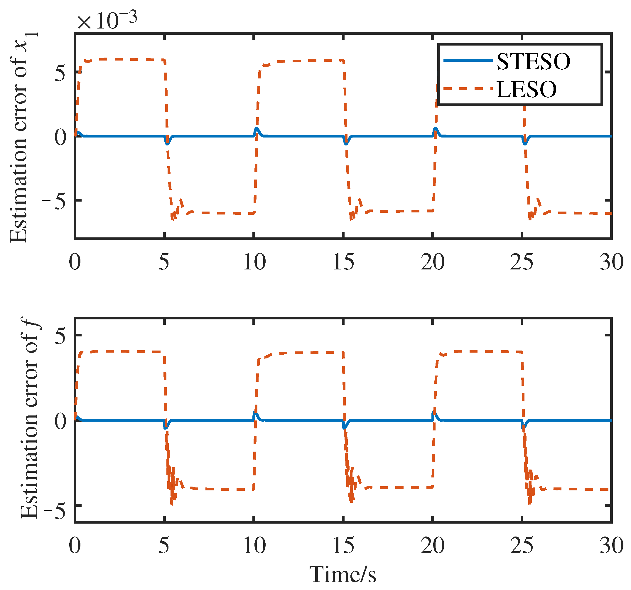
4.1. Ramp Disturbance

For a second-order nonlinear system given by

$$\begin{array}{c}\hfill \left\{\begin{array}{c}{\dot{x}}_1=x_2\hfill \\ {\dot{x}}_2=u+sin\left(x_2{e}^{-2x_1}\right)+x_1^2+x_2^3+x_{1}cos{x}_1+d\hfill \end{array}\right.\end{array},$$

(43)

where $d\left(t\right)=10t$ denotes the ramp external disturbance. Then we have $f=sin\left(x_2{e}^{-2x_1}\right)+x_1^2+x_2^3+x_{1}cos{x}_1+d$, which is second-order differentiable, and $\ddot{f}$ is locally bounded. The control parameters are selected as

$$\begin{array}{c}\hfill \begin{array}{c}{\gamma }_1=64,{\gamma }_2=16,{\beta }_1=45,k_1=40,k_2=15,k_3=40,k_4=957.25,c_1=15.\hfill \end{array}\end{array}$$

(44)

The parameters of the LESO-based controller is also selected as that in (44). The task of the controller is to stabilize system (43) to its origin. The collected simulation results are shown in Figure 1 and Figure 2. Note that this article focuses on the disturbance estimation and compensation problem of STESO, then the analysis of the input is omitted for simplicity. Specifically, when the stable state is achieved, the input of u is the value of the nonlinear term of the controlled model. It can be seen from Figure 1 that the closed-loop system with the proposed method maintains zero tracking error within 1 s, while the output of the system with LESO has a constant tracking error of 0.067. The maximum tracking error of the STESO-based controller is 0.0017, which is much smaller than the comparative one. It can be concluded from the comparison that the proposed method achieves better transient performance and maintains a lower tracking error.

Figure 1. Simulation results of ramp disturbance—system out: controller with STESO (solid line); controller with LESO (dashed line).

Figure 2. Simulation results of ramp disturbance—estimation error: STESO (solid line); LESO (dashed line).

The estimation errors of the proposed and comparative observer are shown in Figure 2. As described in Section 2, the LESO is not able to handle the ramp disturbance. It is seen from Figure 2 that the estimation errors are not attenuated with time. The maximum estimation error of $x_1$ of STESO is about $1.4\times {10}^{-4}$ at 0.16 s, while that of the comparative method is about $3\times {10}^{-3}$, which is 20 times greater than the proposed one. The estimation error of f, the total disturbance, shares the same situation. The maximum estimation errors of STESO and LESO for f are 0.1 and 2, respectively. It can be inferred from the comparison that the proposed observer achieves better performance with less settling time and zero estimation error than the LESO.

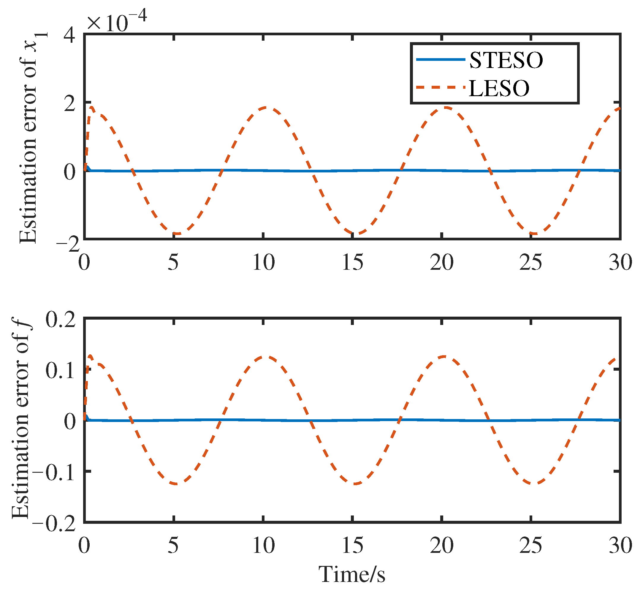
4.2. Sinusoidal Disturbance

The external disturbance in system (43) is defined as $d\left(t\right)=sin\left(0.2\pi t\right)$ in this case. For the continuous and non-diminishing disturbance, our task is to proposed a controller and drive the system to zero with less settling time and smaller tracking error. To this end, the parameters of the STESO-based controller and the comparative one are set according to (44). The comparative simulation results are shown in Figure 3 and Figure 4.

Figure 3. Simulation results of sinusoidal disturbance—system out: controller with STESO (solid line); controller with LESO (dashed line).

Figure 4. Simulation results of sinusoidal disturbance—estimation error: STESO (solid line); LESO (dashed line).

As can be seen from Figure 3, the output of the system with the proposed observer maintains a value of approximately zero. The magnitude of the tracking error is $2.9\times {10}^{-5}$. As a comparison, the performance of the comparative method is also presented. However, the comparative controller achieves the sinusoidal-shaped tracking error with a magnitude of $4.2\times {10}^{-3}$, which has the same frequency as $d\left(t\right)$.

The estimation errors of the simulations are shown in Figure 4. It is seen that the estimation error of $x_1$ of STESO is approximately zero, which vibrates with a magnitude of $1.3\times {10}^{-6}$. It is quite small compared with that of comparative one, which has a magnitude of $1.8\times {10}^{-4}$. It also can be seen from Figure 4 that the estimation errors of f of the proposed and comparative observer are of magnitudes of $8.7\times {10}^{-4}$ and 0.12, respectively.

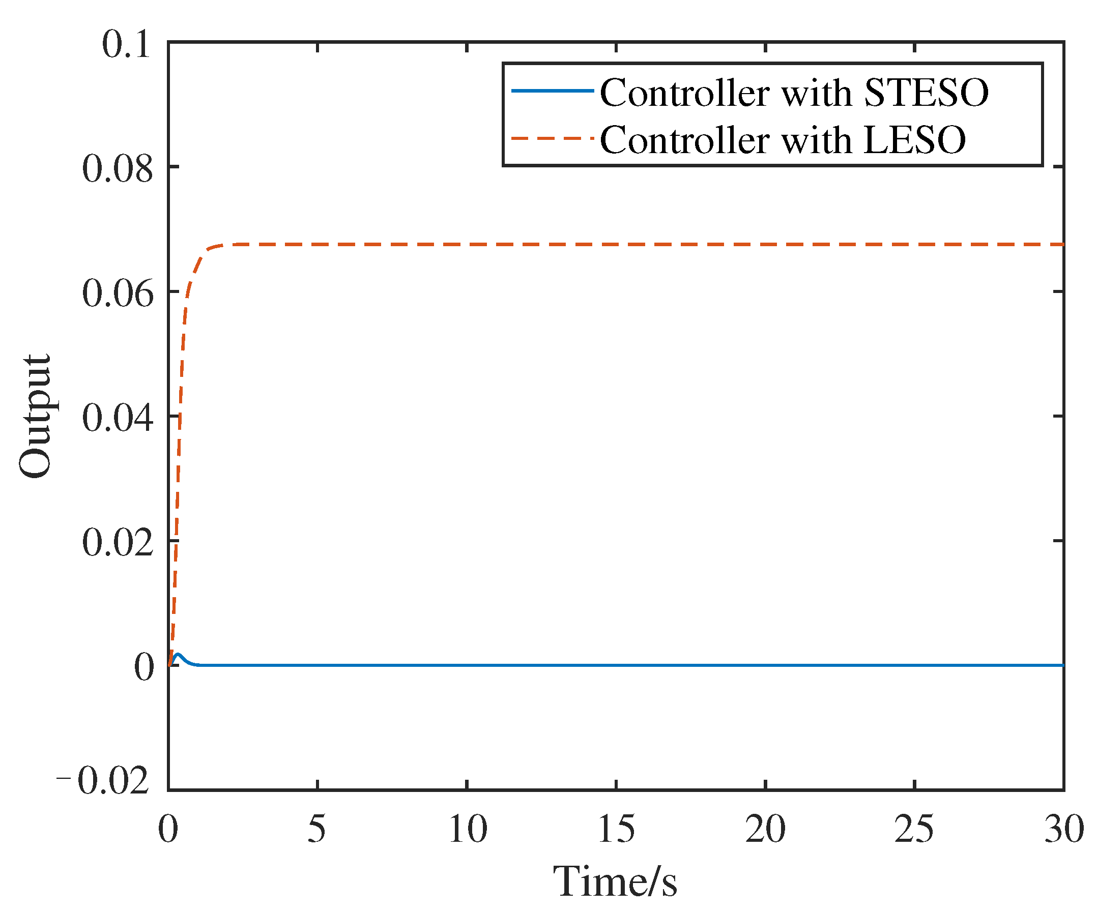
4.3. Robustness Analysis

To verify the robustness, system (43) is modified as

$$\begin{array}{c}\hfill \left\{\begin{array}{c}{\dot{x}}_1=x_2\hfill \\ {\dot{x}}_2=u+sin\left(x_2{e}^{-6x_1}\right)+x_1^4-2x_2^3+x_{1}cos{x}_1+d\hfill \end{array}\right.,\end{array}$$

(45)

where d is the combination of multiple disturbances including sawtooth and sinusoidal wave. The sawtooth disturbance has a magnitude of 100 and the rate of it is 0.1 Hz with respect to time. The sinusoidal disturbance is set as $sin\left(0.1\pi t\right)$. The parameters of the controllers are not retuned. The simulation results are shown in Figure 5 and Figure 6.

Figure 5. Simulation resultsof multiple disturbance—system out: controller with STESO (solid line); controller with LESO (dashed line).

Figure 6. Simulation resultsof multiple disturbance—estimation error: STESO (solid line); LESO (dashed line).

As d is composed of the saw-tooth and sinusoidal disturbances, then the derivative of d contains the pulse function component. The performance of the proposed and comparative controller are under challenge. The system model is modified, and the parameters are unchanged. As shown in Figure 5, the outputs of the system (45) with the proposed and comparative controllers are presented. It is seen that the tracking error of both controllers vibrates when the disturbances are added to d. However, the system with STESO achieves zero tracking error after the oscillations, while the comparative system maintains an error of ±0.13, which will not diminish with time.

The simulation results of the extended observers are shown in Figure 6, which are utilized to verify the robustness and stability of the proposed STESO. As we can see, the estimation errors share the same trend with the tracking error. The estimation error of $x_1$ of the proposed and comparative method are zero and $\pm 5.9\times {10}^{-3}$, respectively. It can also be seen from Figure 6 that the estimation error of f of STESO and LESO are zero and $\pm 4$, respectively. Therefore, it can be inferred from Figure 6 that the proposed observer can maintain zero estimation error for the given multiple disturbance and achieves better performance than the comparative one.

5. Conclusions

In this paper, the super-twisting sliding mode control strategy is applied to improve the performance of extended state observer and the STESO is proposed. Specifically, the proposed method can maintain about zero estimation error in the presence of non-diminishing disturbances, which is a great improvement to the normal extended state observer. The asymptotic convergence of the STESO and asymptotic stability of the closed-loop system are proved by using the Lyapunov method. The convergence time of the sliding manifold of the observer is calculated. Furthermore, the performance of the STESO and related controller are investigated through simulations. Simulation results are presented to show the efficiency and strong robustness of the proposed control strategy at the end of this paper. In our future work, the STESO will be utilized with other control algorithms to further improve the closed-loop performance. We are sure that the proposed method is a promising tool to be expanded to the multi-input–multi-output (MIMO) systems.

References

1. Xie, L.; Guo, L. How much uncertainty can be dealt with by feedback? IEEE Trans. Autom. Control 2000, 45, 2203–2217. [Google Scholar]
2. Gao, Z. On the centrality of disturbance rejection in automatic control. ISA Trans. 2014, 53, 850–857. [Google Scholar] [CrossRef] [Green Version]
3. Chen, W.; Yang, J.; Guo, L.; Li, S. Disturbance-Observer-Based Control and Related Methods—An Overview. IEEE Trans. Ind. Electron. 2016, 63, 1083–1095. [Google Scholar] [CrossRef] [Green Version]
4. Han, J. From PID to Active Disturbance Rejection Control. IEEE Trans. Ind. Electron. 2009, 56, 900–906. [Google Scholar] [CrossRef]
5. Gao, Z. Scaling and bandwidth parameterization based controller tuning. In Proceedings of the American Control Conference, Denver, CO, USA, 4–6 June 2003; pp. 4989–4996. [Google Scholar]
6. Guo, B.; Zhao, Z. On the convergence of an extended state observer for nonlinear systems with uncertainty. Syst. Control. Lett. 2011, 60, 420–430. [Google Scholar] [CrossRef]
7. Xue, W.; Huang, Y. Performance analysis of active disturbance rejection tracking control for a class of uncertain LTI systems. ISA Trans. 2015, 50, 133–154. [Google Scholar] [CrossRef]
8. Zhou, R.; Tan, W. Analysis and Tuning of General Linear Active Disturbance Rejection Controllers. IEEE Trans. Ind. Electron. 2019, 66, 5497–5507. [Google Scholar] [CrossRef]
9. Zhang, Y.; Chen, Z.; Sun, M. Trajectory tracking control for a quadrotor unmanned aerial vehicle based on dynamic surface active disturbance rejection control. Trans. Inst. Meas. Control 2020, 42, 2198–2205. [Google Scholar] [CrossRef]
10. Ran, M.; Wang, Q.; Dong, C. Active disturbance rejection consensus control of uncertain high-order nonlinear multi-agent systems. Trans. Inst. Meas. Control 2016, 42, 604–617. [Google Scholar] [CrossRef]
11. Sun, L.; Zhang, Y.; Li, D.; Lee, K. Tuning of Active Disturdance Rejection Control with application to power plant furnace regulation. Control Eng. Pract. 2019, 92, 104122.1–104122.10. [Google Scholar] [CrossRef]
12. Xie, H.; Li, S.; Song, K.; He, G. Model-based Decoupling Control of VGT and EGR with Active Disturbance Rejection in Diesel Engines. IFAC Proc. Vol. 2013, 46, 282–288. [Google Scholar] [CrossRef]
13. Qiu, D.; Sun, M.; Wang, Z.; Wang, Y.; Chen, Z. Practical Wind-Disturbance Rejection for Large Deep Space Observatory Antenna. IEEE Trans. Control Syst. Technol. 2014, 22, 1983–1990. [Google Scholar] [CrossRef]
14. Yoo, D.; Yau, S.S.; Gao, Z. On convergence of the linear extended state observer. In Proceedings of the 2006 IEEE Conference on Computer Aided Control System Design, 2006 IEEE International Conference on Control Applications, 2006 IEEE International Symposium on Intelligent Control, Munich, Germany, 4–6 October 2006; pp. 1645–1650. [Google Scholar]
15. Yoo, D.; Yau, S.; Gao, Z. Optimal fast tracking observer bandwidth of the linear extended state observer. Int. J. Control 2007, 80, 102–111. [Google Scholar] [CrossRef]
16. Yang, X.; Huang, Y. Capabilities of extended state observer for estimating uncertainties. In Proceedings of the American Control Conference, St. Louis, MO, USA, 10–12 June 2009; pp. 3700–3705. [Google Scholar]
17. Zheng, Q.; Gao, L.; Gao, Z. On stability analysis of active disturbance rejection control for nonlinear time-varying plants with unknown dynamics. In Proceedings of the 2007 46th IEEE Conference on Decision and Control, New Orleans, LA, USA, 12–14 December 2007; pp. 3501–3506. [Google Scholar]
18. Zheng, Q.; Gao, Z. Active disturbance rejection control: Between the formulation in time and the understanding in frequency. Control Theory Technol. 2016, 14, 250–259. [Google Scholar] [CrossRef]
19. Shao, S.; Gao, Z. On the conditions of exponential stability in active disturbance rejection control based on singular perturbation analysis. Int. J. Control 2017, 98, 2085–2097. [Google Scholar] [CrossRef]
20. Ran, M.; Wang, Q.; Dong, C. Stabilization of a class of nonlinear systems with actuator saturation via active disturbance rejection control. Automatica 2016, 63, 302–310. [Google Scholar] [CrossRef]
21. Chen, Z.; Wang, Y.; Sun, M.; Sun, Q. Convergence and stability analysis of active disturbance rejection control for first-order nonlinear dynamic systems. Trans. Inst. Meas. Control 2019, 41, 2064–2076. [Google Scholar] [CrossRef]
22. Shtessel, Y.; Fridman, L.; Zinober, A. Higher order sliding modes. Int. J. Robust Nonlinear Control 2008, 18, 381–384. [Google Scholar] [CrossRef]
23. Levant, A. Sliding Order and Sliding Accuracy in Sliding Mode Control. Int. J. Control 1993, 58, 1247–1263. [Google Scholar] [CrossRef]
24. Defoort, M.; Nollet, F.; Floquet, T.; Perruquetti, W. A Third-Order Sliding-Mode Controller for a Stepper Motor. IEEE Trans. Ind. Electron. 2009, 56, 3337–3346. [Google Scholar] [CrossRef]
25. Haghighi, D.; Mobayen, S. Design of an adaptive super-twisting decoupled terminal sliding mode control scheme for a class of fourth-order systems. ISA Trans. 2011, 75, 216–225. [Google Scholar] [CrossRef] [PubMed]
26. Liu, J.; Sun, M.; Chen, Z.; Sun, Q. Super-twisting sliding mode control for aircraft at high angle of attack based on finite-time extended state observer. Int. J. Control 2020, 99, 2785–2799. [Google Scholar] [CrossRef]
27. Salgado, I.; Chairez, I.; Moreno, J.; Fridman, L.; Poznyak, A. Generalized Super-Twisting Observer for Nonlinear Systems. IFAC Proc. Vol. 2011, 44, 14353–14358. [Google Scholar] [CrossRef] [Green Version]
28. Zong, Q.; Dong, Q.; Wang, F.; Tian, B. Super twisting sliding mode control for a flexible air-breathing hypersonic vehicle based on disturbance observer. Sci. China Ser. F Inf. Sci. 2015, 58, 1–15. [Google Scholar] [CrossRef] [Green Version]
29. Chalanga, A.; Kamal, S.; Fridman, L.; Bandyopadhyay, B.; Moreno, J. Implementation of Super-Twisting Control: Super-Twisting and Higher Order Sliding-Mode Observer-Based Approaches. IEEE Trans. Ind. Electron. 2016, 63, 3677–3685. [Google Scholar] [CrossRef]
30. Bhat, S.; Bernstein, D. Finite-time stability of continuous autonomous systems. SIAM J. Control Optim. 2000, 38, 751–766. [Google Scholar] [CrossRef]