Article

Deep Learning Approaches to Automatic Chronic Venous Disease Classification

1
Institute of Precision Mechanics and Control of the Russian Academy of Sciences, 24, ul. Rabochaya, 410028 Saratov, Russia
2
R&D Department, TOO Fle, Office 20, 24, st. Panfilova, Almaty 050000, Kazakhstan
3
Omega Clinic, 46, ul. Komsomolskaia, 410031 Saratov, Russia
*
Author to whom correspondence should be addressed.
Mathematics 2022, 10(19), 3571; https://doi.org/10.3390/math10193571
Submission received: 26 August 2022 / Revised: 18 September 2022 / Accepted: 27 September 2022 / Published: 30 September 2022
(This article belongs to the Special Issue Recent Advances in Artificial Intelligence and Machine Learning)

Abstract

:
Chronic venous disease (CVD) occurs in a substantial proportion of the world’s population. If the onset of CVD looks like a cosmetic defect, over time, it might be transformed into serious problems that will require surgical intervention. The aim of this work is to use deep learning (DL) methods for automatic classification of the stage of CVD for self-diagnosis of a patient by using the image of the patient’s legs. The images of legs with CVD required for DL algorithms were collected from open Internet resources using the developed algorithms. For image preprocessing, the binary classification problem “legs–no legs” was solved based on Resnet50 with accuracy of 0.998. The application of this filter made it possible to collect a dataset of 11,118 good-quality leg images with various stages of CVD. For classification of various stages of CVD according to the CEAP classification, the multi-classification problem was set and resolved by using four neural networks with completely different architectures: Resnet50 and transformers such as data-efficient image transformers (DeiT) and a custom vision transformer (vit-base-patch16-224 and vit-base-patch16-384). The model based on DeiT without any tuning showed better results than the model based on Resnet50 did (precision = 0.770 (DeiT) and 0.615 (Resnet50)). vit-base-patch16-384 showed the best results (precision = 0.79). To demonstrate the results of the work, a Telegram bot was developed, in which fully functioning DL algorithms were implemented. This bot allowed evaluating the condition of the patient’s legs with fairly good accuracy of CVD classification.

1. Introduction

Chronic venous disease (CVD) is a disease that affects a substantial number of the population [1,2]. In the initial stages of CVD, patients do not take this disease seriously and prefer to think of it as a cosmetic defect. However, further development of CVD may require a surgical intervention, the cost of which can be quite high [3,4]. At the same time, it is possible to slow down the development of the disease in the early stages using compression or pharmacological therapy or by reducing risk factors such as obesity and prolonged standing or sitting [5].
The problem of using neural networks in the task of diagnosing the stage of varicose veins has long been of interest to researchers. Bailey et al. [6] described the process of splitting the stages of varicose disease into classes for a neural network and one of the first methods for applying a neural network to the image classifying problem of legs with varicose veins. However, the level of technological and algorithmic progress of that time did not allow transferring the ideas expressed in that work to life.
Furthermore, with the development of technologies and developments in the field of machine learning (ML) and deep learning (DL), more and more advanced methods for data and image processing have been designed [7,8,9,10]. The specifics of ML and DL models for medicine problems, the main problems of these models, and the difficulties and potential risks of using them are discussed in [7]. Bharati et al. [8] discussed various approaches to solving recognition problems for X-ray, CT scan, ultrasound, and MRI images. Zhou et al. [9] reviewed the state, main trends, and development prospects of DL in medicine at the time of 2020–2021. The study highlighted the areas where significant progress has been achieved, such as segmentation of anatomical structures, detection and diagnosis in chest radiography, decision support in lung cancer screening, COVID-19 case studies, neuroimage segmentation and tissue classification, deformable image registration, neuroimaging prediction, GANs in neuroimaging, cardiac image segmentation, cardiac motion tracking, cardiac vessel segmentation, organs and lesions, opportunistic screening, nuclei detection and segmentation, disease grading, mutation identification and pathway association, and survival and disease outcome prediction.
Wang et al. [11] developed an automated system for predicting the interaction of drugs with targets using one of the recurrent neural networks—the Deep Long Short-Term Memory (DeepLSTM). The prediction results were compared with those of multilayer perceptron (MLP) networks, in which the number of hidden layers and neurons is the same as in the DeepLSTM network, and with those of a Support Vector Machine (SVM) with parameters that were optimized by a grid search technology. The authors showed [11] that DeepLSTM outperforms traditional ML systems for the problem under consideration in terms of the area under the Receiver Operating Characteristic curve (AUC).
ML and DL algorithms have proven to be effective for diagnosing COVID-19 based on the analysis of various types of data and images [12,13,14,15]. The quality of the solution obtained as a result of ML and DL models significantly depends on the chosen neural network, its parameters, and the completeness of the dataset. For example, Qu et al. [12] used YOLOv5 for the task of abnormality detection in a chest radiograph. The authors in [12] got the [email protected] (mean average precision) metrics for their decision higher by 0.157 and 0.101 than those of Faster RCNN and EfficientDet, respectively. Saxena et al. [13] described the results of the development of a COVID-19 classifier using convolutional neural networks on chest X-ray images. The model was trained on the ChestX-ray14 dataset [16], which contains 112,120 frontal chest radiograph images from 30,805 unique patients. As a result, the model had an accuracy of 0.9263 on the validation dataset and demonstrated a better result than the average results of four radiologists.
DL models can show outstanding results, but they require computers with great computational power and specialized hardware for model training, which makes it difficult to create model prototypes and make them portable. Ali et al. [17] modified U-Net image segmentation models for an Intel Neural Compute Stick [18]. Three datasets were used in [17]: BraTs dataset of brain MRI, a heart MRI dataset [19], and the Ziehl–Neelsen sputum smear microscopy image (ZNSDB) dataset [20]. The parameters for the modified U-Net were reduced to 0.49 million, whereas the classic U-Net used 30 million, and Intel’s Model used 7.85 million parameters. The test time was 123 msec on the Neural Compute Stick and 61 msec on Intel’s Model and the modified U-Net. The highest dice score was almost equal for all models (0.97 for the classical U-Net and 0.9625 for Intel’s Model and the modified U-Net).
One more problem of DL models in medicine is that the images in the training dataset must be labeled, and the process of labeling requires clinical expertise, which is time- and resource-consuming [21]. Chi et al. [22] suggested an approach for image autosegmentation based on generation of pseudocontours by utilizing deformable image registration to propagate atlas contours onto abundant unlabeled images.
Despite the above-mentioned problems, DL and ML models are also widely used in phlebology. Butova et al. [23] reviewed the current level of using ML and DL models to solve different problems in phlebology such as the prediction or classification of arterial disease, venous thromboembolism, and chronic venous disease. Ryan et al. [24] used gradient boosted machine learning algorithms to predict deep venous thrombosis at 12 and 24 h prior to onset. The resulting model was trained on 99,237 general ward or ICU patients. The quality of the model was 0.83 based on AUROC (Area Under the Receiver Operating Characteristics). A machine learning approach was used by Nafee et al. in [25] to predict venous thrombosis in acute medically ill patients based on different patients’ characteristics. The accuracy of the model was 0.711. Fong-Mata et al. [26] proposed a new back-propagation artificial neural network model and a data augmentation algorithm for synthetic cases generation. Therefore, the dataset included 10,000 synthetic cases. The proposed model was validated by performing the k-fold cross validation technique using a processed dataset. The test was performed by using 59 real cases obtained from a regional hospital, with 98.30% accuracy.
Risk assessment models in phlebology are being actively developed [27,28,29]. Rosenberg et al. [27] did an external validation of the International Medical Prevention Registry on Venous Thromboembolism for a risk assessment model in a hospitalized general medical population. Barbar et al. [28] used ML approaches to adapt a risk assessment model for the identification of hospitalized medical patients at risk for venous thromboembolism to permit identification of all conditions for which the latest international guidelines strongly recommend thromboprophylaxis. Hippisley-Cox et al. [29] developed and validated an unprecedented clinical risk prediction algorithm to estimate individual patients’ risk of venous thromboembolism. The authors used an extensive dataset to study problems related to phlebology. The derivation cohort included 14,756 incident cases of venous thromboembolism from 10,095,199 person years of observation (rate of 14.6 per 10,000 person years). The validation cohort included 6913 incident cases from 4,632,694 person years of observation (14.9 per 10,000 person years). As a result, this work presented a new risk prediction model that quantifies absolute risk of thrombosis at 1 and 5 years.
Since venous thromboembolism is a common complication of cancer, but the risk of developing venous thromboembolism varies greatly among individuals, cancer patients form a particular cohort that needs a special study of risk prediction features for venous thromboembolism [30,31,32]. Es et al. [30] compared risk prediction scores for venous thromboembolism in cancer patients. Ferroni et al. [31] developed a set of venous thromboembolism risk predictors in cancer patients using kernel machine learning and random optimization techniques. Pabinger et al. [32] constructed a very simple prediction model of the risk of venous thromboembolism in ambulatory patients with solid cancers, and this model consists of only one clinical factor (tumor-site category) and one biomarker (D-dimer).
Therefore, the current level of progress in artificial intelligence and deep learning algorithms makes it possible to develop applications for self-diagnosis of patients, so that they can determine the level of CVD themselves and consult a doctor on time.
A number of works have already been published on determining the severity of CVD using artificial intelligence. Zhu et al. [33] described the architecture of a model inspired by popular neural networks such as Google-Net and VGG. This model, with a detailed description of the mathematical functionality of each of the layers, according to the study, shows good results in diagnosing the stage of varicose veins using an image. In addition, that work demonstrates the result of working on a problem with various popular machine learning algorithms (for example, k-means) and making a comparative analysis with them. Atreyapurapu et al. [34] solved a binary classification problem of whether a chronic venous insufficiency exists or not. The authors studied 50 patients and their 5200 images from magnetic resonance venograms. These images were processed with the Google collaboratory network to train a 121-layer dense-net convolutional neural network. The CEAP (clinical, etiology, anatomy, pathophysiology) classification was used as it is globally accepted and widespread. The CEAP classification contains seven stages of CVD [35]: C0 (normal legs with no visible signs of CVD), C1 (spider and reticular veins), C2 (varicose veins, which have a diameter of 3 mm or more), C3 (edema), C4 (skin and subcutaneous tissue changes secondary to CVD), C5 (healed venous ulcer), C6 (active venous ulcer).
The accuracy of distinguishing between normal (C0–C2) and abnormal (C3–C6) images was about 97%. Classes C3–C6 of CVD can be considered as chronic venous insufficiency according to the CEAP classification [35].
Shi et al. [36] described the results of the development of an automated system for classifying CVD conditions as mild, moderate, and severe. The system was trained on 271 photos taken by certified doctors of vascular surgery, and the background of the photographs was uniform. The Bag of Visual Words [37] was used as a neural network. The authors claim very good accuracy of the resulting model (up to 0.95 for mild, 0.89 for moderate, and 0.95 for severe). However, the requirements for images, like a certain position of the leg in the photo or a uniform background, make it difficult to use it in practice for self-diagnosis of patients.
Therefore, the creation of an automated system for self-diagnosis of patients that does not have strict requirements for the quality of feet photographs remains an actual problem.
The aim of this work is to develop a system which can predict the degree of CVD for the self-diagnosis of patients using deep learning algorithms. To achieve this goal, the following stages were completed:
1. Data mining of images of men’s and women’s legs with varying degrees of CVD, not including those with wounds and tattoos.
2. Developing a “legs–not legs” filter so that only legs get into the main classification algorithm. This is a very important step since classification image models require much more computational resources than a simple “object–not object” image filter.
3. Developing a classifier of CVD degrees according to the CEAP classification. Neural networks of various architectures such as ResNet50 and Transformers [38,39] were used. The use of ResNet50 was due to its widespread use for image classification problems. Transformers are one of the newer neural networks that have already proven their worth in medical imaging [40,41].
The rest of the paper is structured as follows: Section 2 describes the process of data gathering, the datasets, the proposed models, and the methods. Section 3 presents the conducted experiments. Section 4 discusses the study’s findings and results. Section 5 draws the main conclusion of the work.

2. Materials and Methods

2.1. Data Mining

One of the main problems of classification tasks solved using deep learning algorithms is collecting enough quantity high-quality images for each of the predicted classes. In addition, it is desirable that each class contains approximately the same number of images.
To solve these problems, we can use open databases with verified medical images or conduct a study in medical institutions and thus collect the image dataset. However, for many medical problems, there are no datasets with the needed images, and gathering the necessary number of images takes too much time.
In this case, data mining of images from open Internet sources, such as Instagram or Google images, can help collect the necessary number of images.
Our data-mining process included several stages that differed specifically in image collection ways. Two “spider” scripts were developed. The first one was developed using Scrapy, which is a fast, open-source web crawling framework written in Python for extracting data from the web pages [42]. This script was used to get images from Instagram accounts. The second spider was developed using Selenium and was used in the Chrome browser to get images from Google. Selenium is a Python web-driver that allows an emulation of real user behavior on web pages [43].

2.1.1. Scrapy Data Mining

In the first stage, about 300 Instagram accounts with many images of legs with CVD were selected for data mining. After 67,000 images were collected, no-legs and low-quality images were removed by hand. There were 10,618 remaining images that showed legs with varying degrees of CVD. Thus, we got our dataset “legs with CVD”.
In order to prevent manual work on separating images with and without legs in the future, a filter “leg–no leg” was trained using Resnet50 [44]. Since the no-legs images contained too many objects and some were of poor quality, an open Flickr Image dataset [45] containing more than 30,000 annotated images was used to solve the binary classification problem and train the “legs–not legs” filter. From the Flickr Image dataset, 11,000 images were taken for the “not legs” category. The dataset “legs–no legs” was used to solve the problem of binary classification based on Resnet50.

2.1.2. Selenium Data Mining

The dataset “legs with CVD” was classified by a certified phlebologist into 7 CEAP classes—from C0 to C6. The C0 class contained practically no images. Therefore, it was necessary to find and add more images with healthy legs.
Therefore, we developed and ran the Selenium spider in the Chrome browser in order to find images of healthy legs through search queries in the Google search engine to fill the C0 class. We collected about 90 000 images, but only 10% of them were unique.
The unique images were passed through the “legs–no legs” filter, and we got only 400 images with healthy legs. These images were added to the C0 class of the dataset “legs with CVD”.
Thus, we had collected the dataset “legs with CVD” of 11,118 images with different degrees of CVD.

2.1.3. Datasets

The dataset “legs–no legs” consisted of 10,618 images of legs and 11,000 images of non-legs. Examples of “leg” images that were obtained by the data-mining process are shown in Figure 1 and Figure 2.
The “leg” images set consisted of different kind of legs: male and female; with or without scars, hair, tattoos; etc.
The final dataset “legs with CVD” consisted of 11,118 images with different degrees of CVD. Example of images of legs with CVD from this dataset are shown in Figure 3.
All 11,118 images of legs were categorized by a certified phlebologist into 7 CEAP classes (C0–C6). After classification, the distribution of images by CEAP classes was: C0—872, C1—2810, C2—1493, C3—3743, C4—1530, C5—403, C6—267. The ratio of the number of images in each class to the total number of images in the dataset is shown in Figure 4.
As can be seen in Figure 4, the dataset “legs with CVD” was significantly unbalanced in contrast to the dataset “leg–not leg”. This must be taken into account when choosing metrics to evaluate the quality of classification results.

2.2. Neural Networks

2.2.1. Filter “Legs–No Legs”

The dataset “legs–no legs” was split into training and validation parts in the proportion 80/20%.
As the baseline for this binary classification problem, a pre-trained ResNet50 model (a residual neural network with 50 layers) [46] from the PyTorch library [47] was chosen.
ResNet is one of the most cited and most popular artificial neural networks for image classification problems. The fundamental difference between ResNet and classical convolutional neural networks is shortcut connections. It means that some images process through all ResNet layers, but the rest skip some layers. Therefore, ResNet is not a fully connected network, and large numbers of layers do not overfit the model and do not reduce accuracy, unlike in classical CNNs.
As the dataset “legs–no legs” contained two well-balanced classes “legs” and “no-legs”, the quality of prediction was evaluated by the accuracy metric, which is the ratio of the number of correct predictions to the total number of predictions—correct and incorrect.

2.2.2. Multi-Classification Problem

To solve the problem of classification according to the degree of CEAP, the following neural networks were chosen: Resnet50, data-efficient image transformers (DeiT), and custom vision transformer (vit-base-patch16-224 and vit-base-patch16-384). ResNet50 and the transformers have different architectures. If ResNet50 is a variant of a convolutional network, then Transformers can be considered as a variant of Graph Neural Networks. The metrics of the models based on Resnet50, DeiT, vit-base-patch16-224 (ViT224), vit-base-patch16-384 (ViT384) were compared to choose the best solution.
Since the imbalance of classes was clearly traced, as can be seen in Figure 4, the accuracy could be misleading. Thus, according to many works, such as [48], the following metrics had to be used for the evaluation of the quality of classification models for the imbalanced dataset:
  • Precision = TruePositive/(TruePositive + FalsePositive)
  • Recall = TruePositive/(TruePositive + FalseNegative)
  • F-Measure = (2 × Precision × Recall)/(Precision + Recall)
  • Logistic Loss curve.
A rated confusion matrix was also built according to the scheme:
Predicted
PositiveNegative
Actual PositiveRated TP =
TruePositive/ActualPositive
Rated FN =
FalseNegative/ActualPositive
NegativeRated FP =
FalsePositive/ActualNegative
Rated TN =
TrueNegative/ActualNegative
where TruePositive—the number of images which were classified correctly, FalseNegative—the number of images that should have been assigned to this class but were not, FalsePositive—the number of images that were erroneously assigned to this class, TrueNegative—the number of images correctly marked as not being in this class; ActualPositive—the number of all images that are actually in this class, ActualNegative—the number of all images that are actually not in this class.
The Logistic Loss (LogLoss) curve is defined as:
l o g l o s s = 1 N i = 1 N j = 1 C a i j log p i j
a i j = { 1 ,   i f   o b j e c t   i   b e l o n g s   t o   c l a s s   j 0 ,   o t h e r w i s e  
where N—the number of images, C—the number of classes, p i j —the probability of classifying object i to class j.

3. Results

3.1. Resnet50 for Filter “Legs–No Legs”

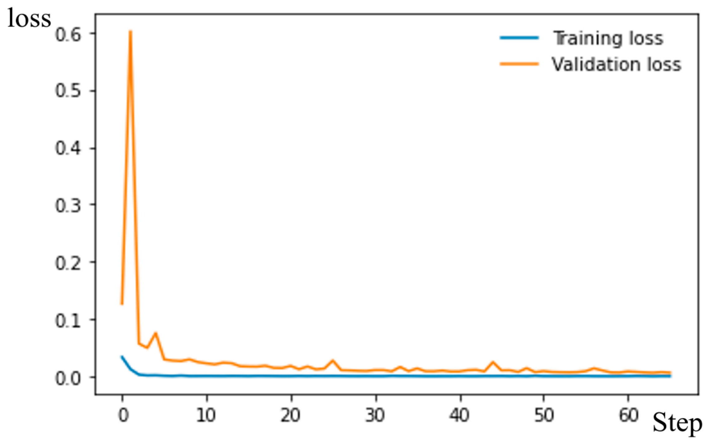
The deep learning model based on Resnet50 for the binary classification problem was trained for one epoch and 60 steps. The LogLoss value reached a constant value close to zero around the fifth step (Figure 5).
As can be seen in Figure 5, the model was not overtrained since the validation log loss curve decreased up to 25 step and then tended asymptotically to a constant value. The accuracy was 0.998, which was a good result for binary classification problems on a well-balanced dataset.

3.2. Resnet50 for the Multi-Classification Problem

For this problem, the model based on Resnet50 was trained for twenty epochs. The training parameters had default values.
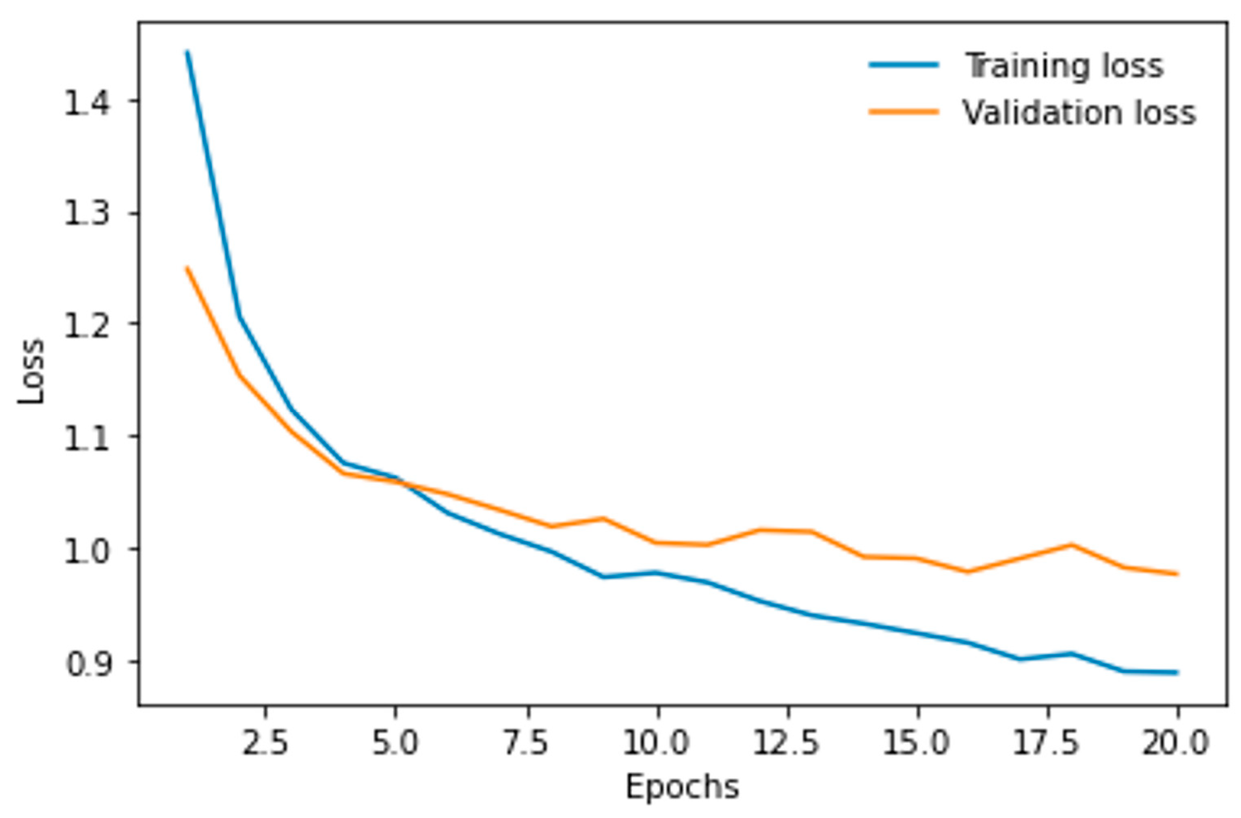
Although the learning curve of logistic loss was slowly decreasing, further training was not advisable since the validation LogLoss curve had reached a nearly constant value (Figure 6).
As can be seen in Figure 6, the model was also not overtrained because validation LogLoss was decreasing. However, the loss values were still too big.
The metrics were not good enough, precision was 0.615, recall was 0.614, and the F1 metric was 0.611. To identify the problems in classification, rated confusion matrices were constructed for each CEAP class (Figure 6).
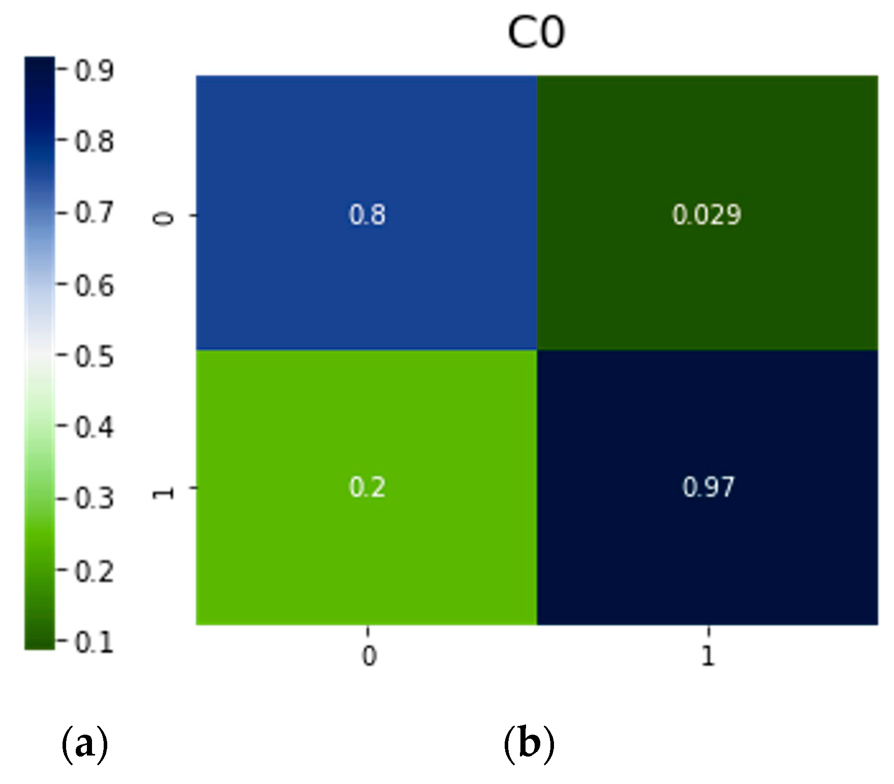
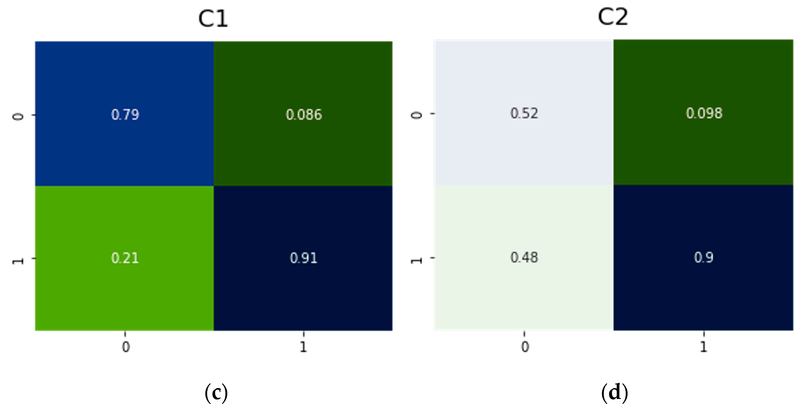
The rated confusion matrices for each CEAP class for the multi-classification model based on Resnet50 are shown in Figure 7 and Figure 8.
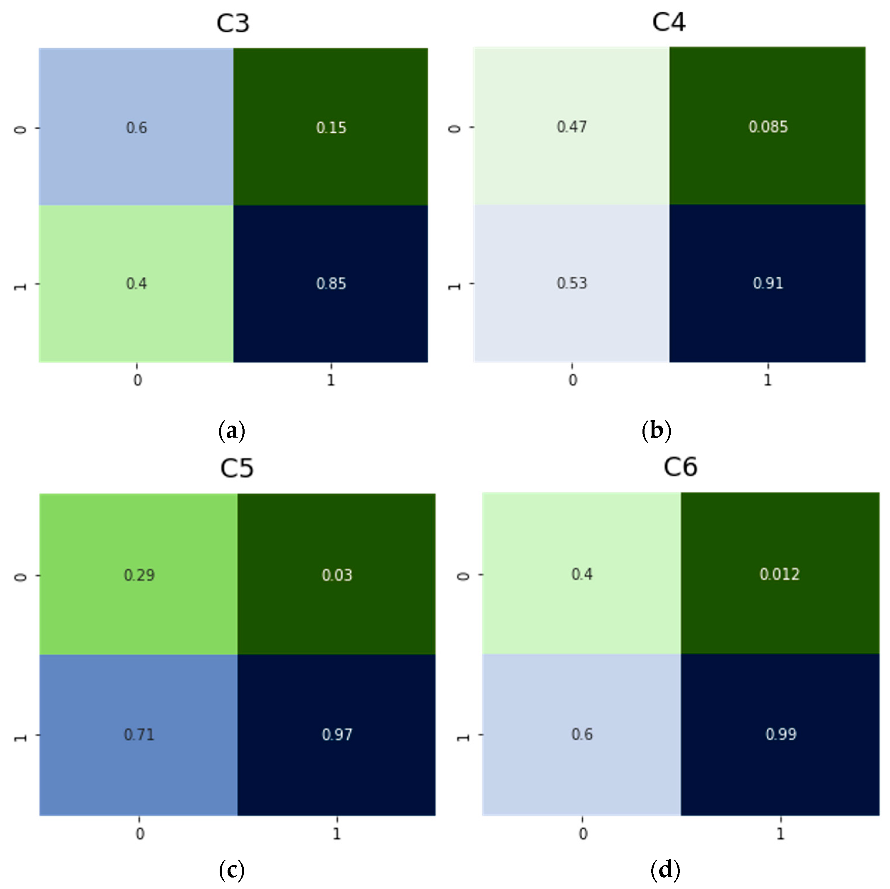
As can be seen in Figure 7 and Figure 8, the model based on Resnet50 predicted that an image did NOT fit into a certain class well enough with a probability of at least 0.85 (for C3) and with a probability of over 0.97 for classes C0, C5, and C6.
However, the model did not perform well in predicting that an image belonged to a certain class. Therefore, we had the probability near 0.8 that the image will be correctly classified only for classes C0 and C1. This was a fascinating result, since C0 contained only 7.84% of the total number of images in the dataset.
The probabilities of correctly assigning an image to classes C2 or C3 were almost equal to the probabilities of making a Type I error (for C2: 0.52 and 0.48; for C3: 0.6 and 0.4). However, it should be noted that the probability of correct classification equal to 0.6 for the multi-classification problem could be considered as a fairly good result.
The probability of making a Type I error for C4, C5, and C6 classes was higher than the probability of correctly classifying an image in these classes. The worst case was for C5, where the probability of a Type I error was 0.71, and the probability of correct classification was only 0.29.
The probability of a Type II error did not exceed 0.1 for all classes, except for C3, for which it was equal to 0.15.
Thus, the quality of the classification could not be considered acceptable. However, since there were no ways to significantly increase classification accuracy based on the constructed model, it was decided to use a different, a more complex neural network, such as Visual Transformers.

3.3. ViT Transformers

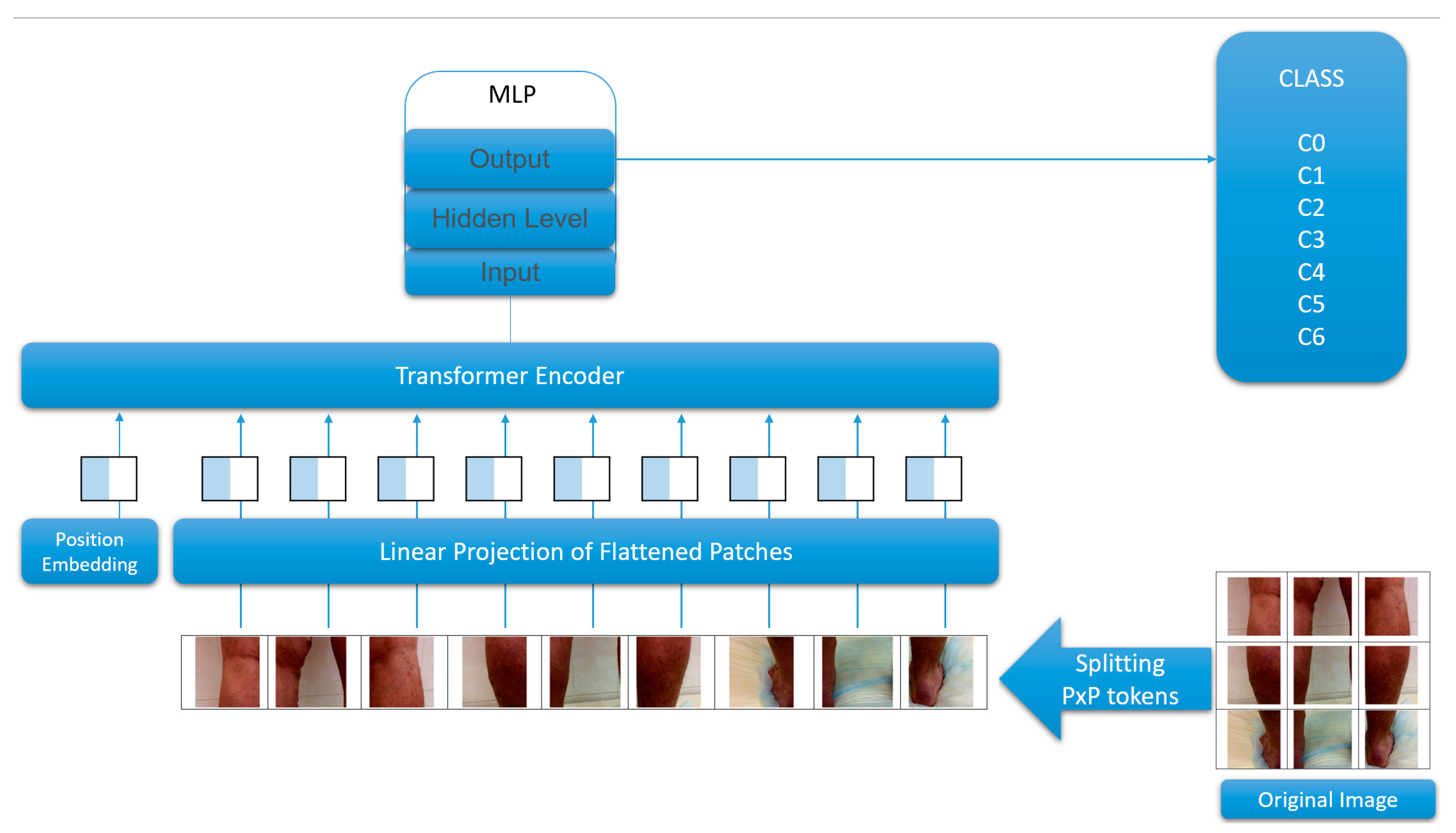
Visual Transformers [38] are outstanding algorithms that made it possible to achieve adequate computational cost just because they use pieces of a picture of a certain size P instead of pixels like convolutional neural networks do. Therefore, the computational complexity significantly is reduced for ViT. Moreover, ViT algorithms are one of the most accurate neural networks for classification problems. The architecture of ViT transformer neural networks is shown in Figure 9.
The main idea of ViT is to use not pixels as layers, but fixed-size image pieces called patches or tokens (Figure 9). Then, the image pieces have to be flattened and mapped to D dimensions with a trainable linear projection, where D is the constant size of the hidden vector of all Transformer layers. The output of this projection is called patch embeddings. Then, a learnable class embedding has to be appended to the sequence of embedded patches. Only this class embedding will be used to predict the output. To handle the positional information of the image patches, a 1D position embedding must be added to the patch embeddings. Without the position embedding, the Transformer Encoder is a permutation-equivariant architecture. Two versions of ViT transformers were used in this work—vit-base-patch16-224 and vit-base-patch16-384. The training parameters for vit-base-patch16-224 and vit-base-patch16-384 are shown in Table 1. The remaining parameters had default values.
The parameters in Table 1 have the following meaning: hidden_size—dimensionality of the encoder layers and the pooler layer, image_size—the resolution of each image, num_hidden_layers—number of hidden layers in the Transformer encoder, patch_size – the resolution of each patch.
As can be seen from Table 1, all parameters for vit-base-patch16-224 and vit-base-patch16-384 were the same except “image_size”. The patch sizes for both versions were 16 × 16 px. However, vit-base-patch16-224 works with a 224 × 224 px tensor, and vit-base-patch16-384 works with a 384 × 384 px tensor. Therefore, we had 196 and 576 tokens in vit-base-patch16-224 works and vit-base-patch16-384 works, respectively.
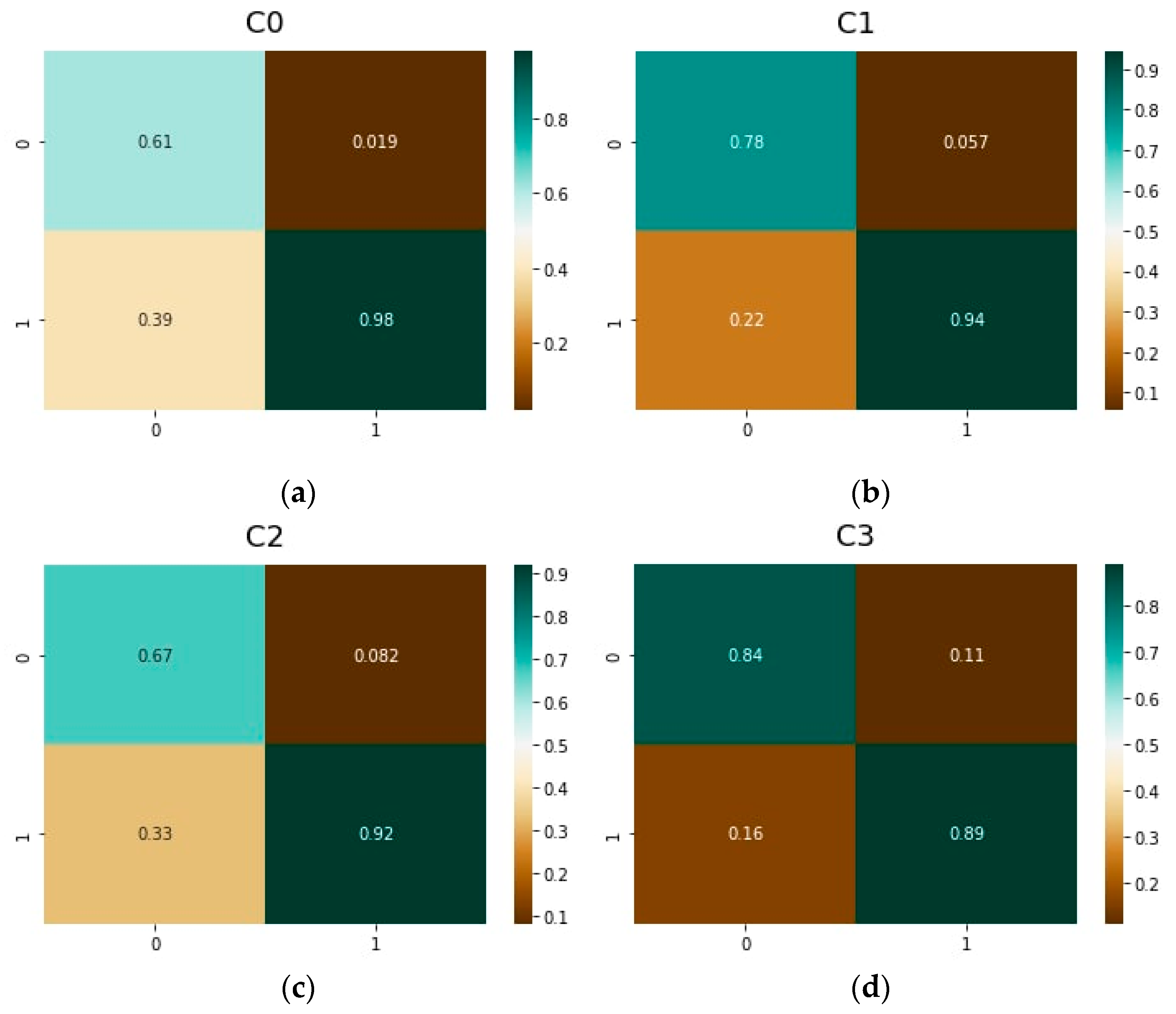
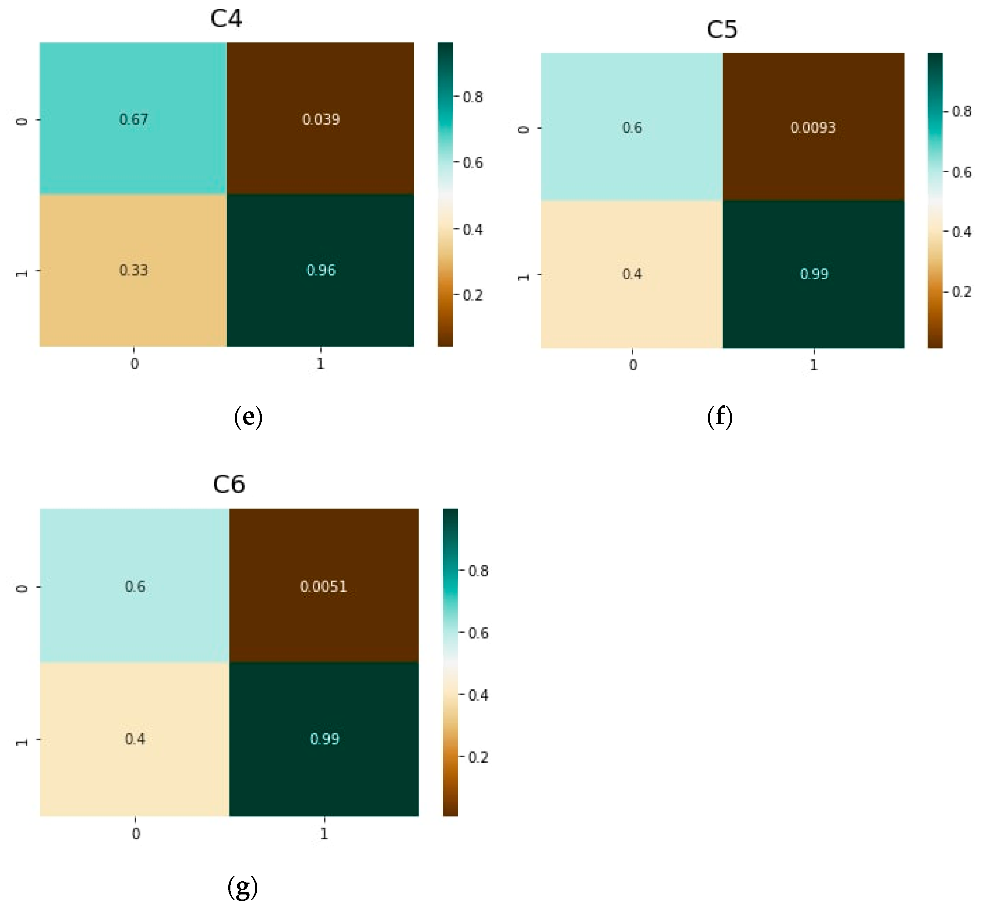
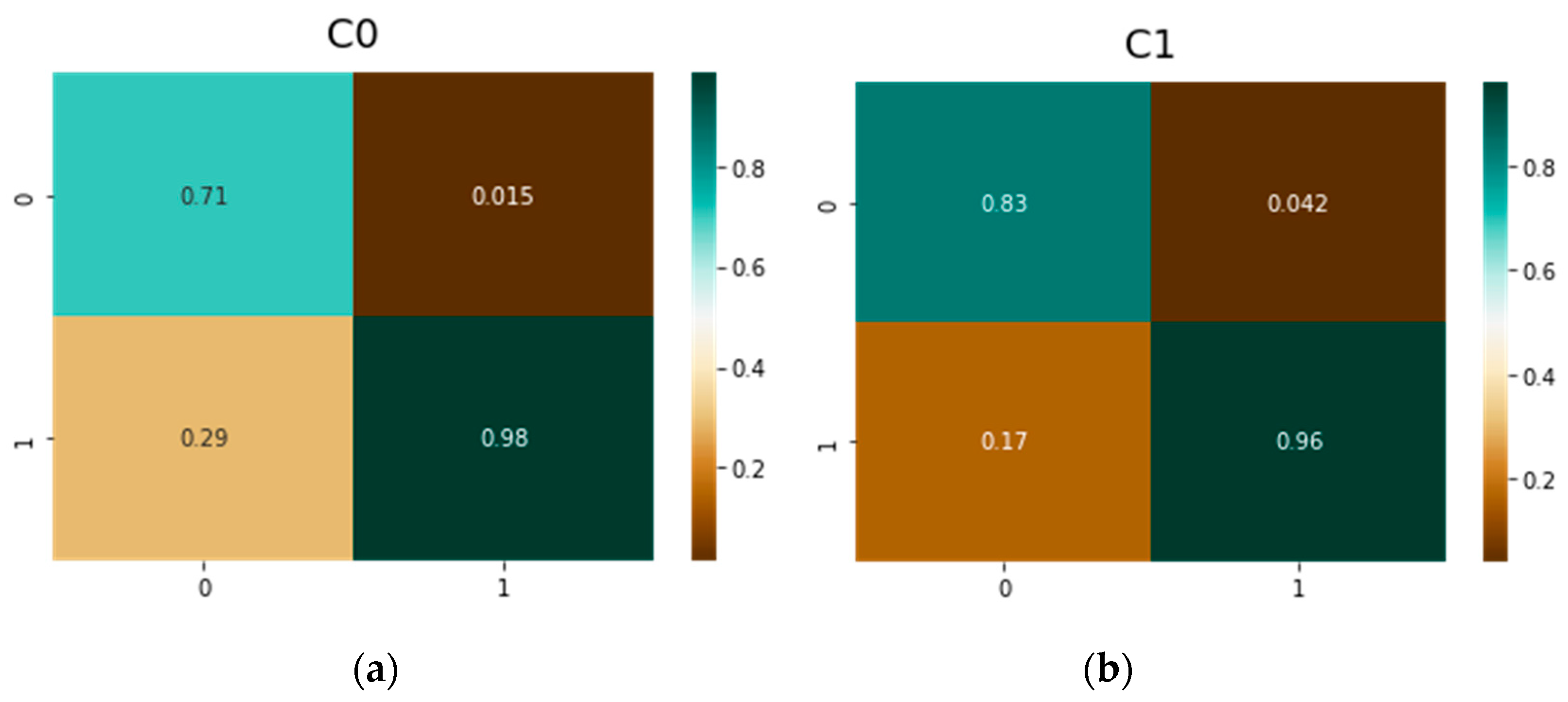
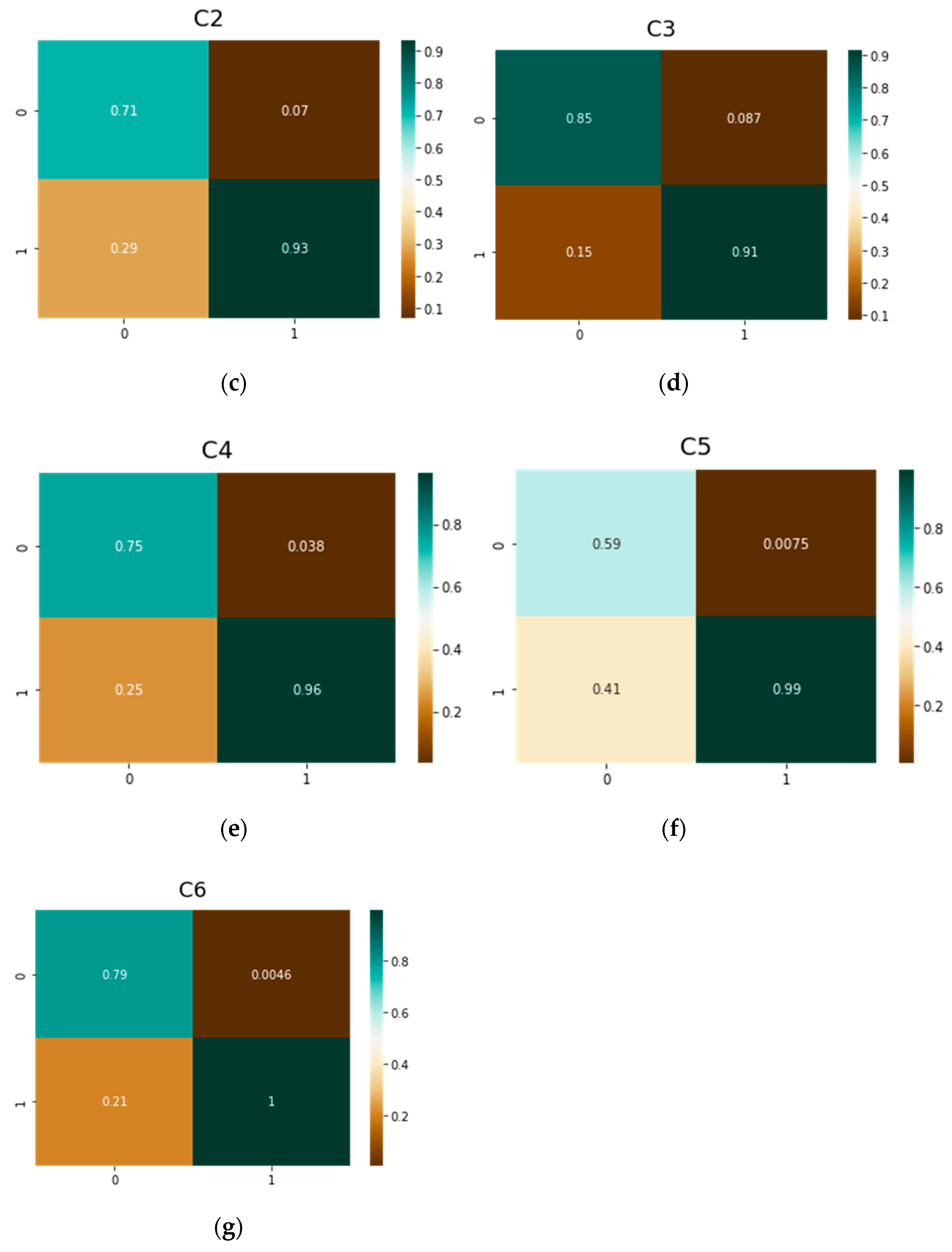
The confusion matrixes for both of these neural nets are shown in Figure 10 and Figure 11.
The metrics for vit-base-patch16-224: precision—0.75, recall—0.75, F1 score—0.75. The metrics for vit-base-patch16-384: precision—0.79, recall—0.79, F1 score—0.79.

3.4. DeiT Multi-Classification Problem

The next transformer model we trained was DeIT (data-efficient image transformers), since it can be considered a light version of ViT. DeIT uses a knowledge distillation procedure specific to vision transformers, when one neural network (the student) trains on the output of another network (the teacher). Therefore, DeiT is just a normal ViT with an additional distillation token.
The deep learning model based on DeiT for the multi-classification problem was trained for twenty epochs, the same as the model based on Resnet50.
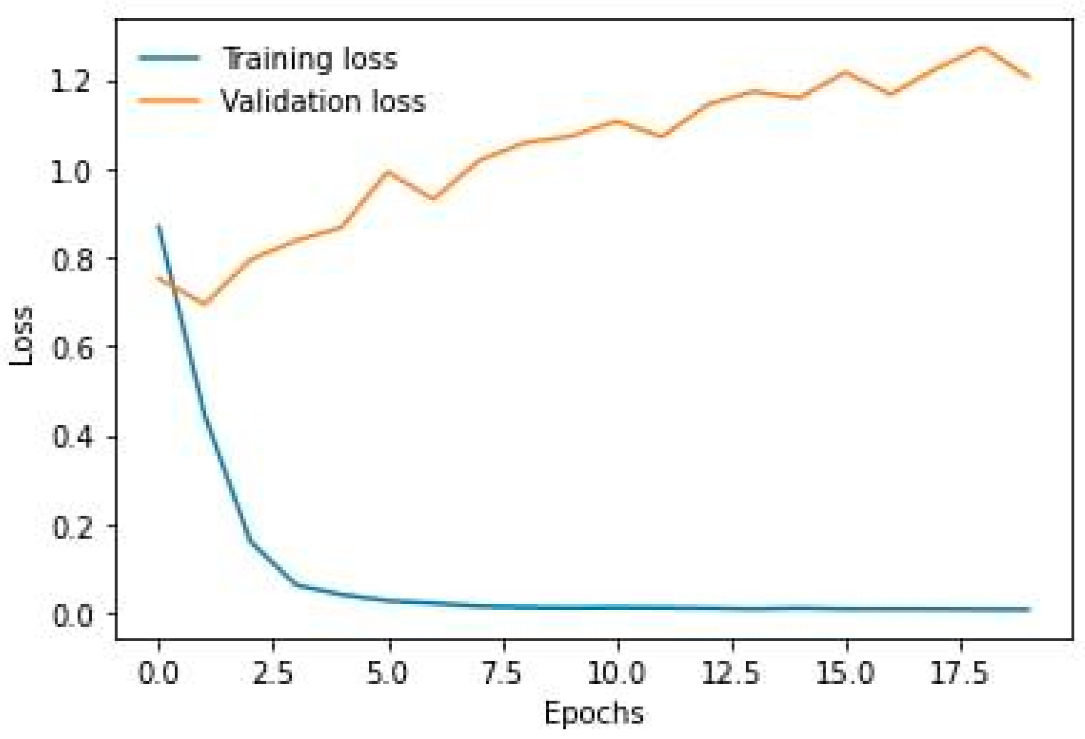
The LogLoss curves for training and validation sets are shown in Figure 12.
As can be seen in Figure 13, the model was overtrained after two epochs because the validation LogLoss curve was increasing after the second epoch. Therefore, the weights of the model that was trained on the second epoch were taken for the classification model.
The metrics were much better than for the model based on Resnet50. The precision was 0.770, the recall was 0.766, and the F1 metric was 0.768.
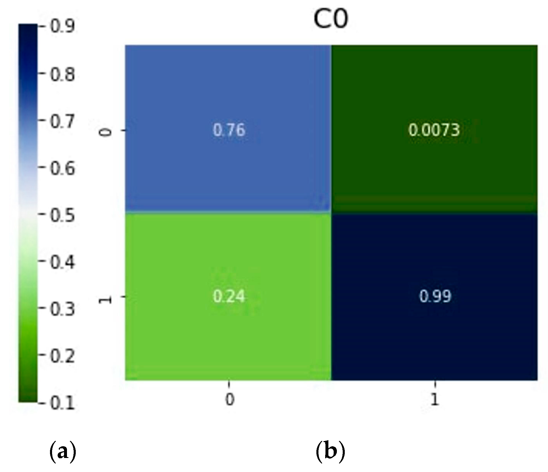
The rated confusion matrices which were constructed for each CEAP class for this model are shown in Figure 13 and Figure 14.
As can be seen in Figure 13 and Figure 14, the classification accuracy improved significantly for almost all classes in comparison to that with Resnet50. The probability of correct classification that an image did not fit the class was not lower than 0.95 for all CEAP classes. It was equal to 0.99 for C0, C5, and C6.

4. Discussion

The main metrics for all trained models are shown in Table 2. The probabilities of classification for each CEAP class obtained in the considered neural networks models are shown in Table 3.
As can be seen in Table 2, the vit-base-patch16-384 model had the best metrics. However, the DeiT model had very similar metrics. That is very important for practical use since vit-base-patch16-384 requires more computational resources for training and prediction than does DeiT, which can be considered a lighter version of ViT models.
The model based on DeiT coild classify an image as C0, C1, and C3 very well, quite well as C2 and C4, and not very well as C5 and C6. Further improvement of the model is needed (Table 3). This model improvement can be made by increasing the quantity of images in the training dataset for classes C5 and C6 and by tuning the model based on DeiT.
The vit-base-patch16-384 model showed the best results in classification for classes C5 and C6 (rated true positive values = 0.59 and 0.79, respectively). However, DeiT worked better than vit-base-patch16-384 for the classification of classes C0 and C1.
The models based on transformers models showed better results than the model based on Resnet50 did for the multi-classification problem of CVD into C1–C6 CEAP classes. On the other hand, the filter “legs–no legs” was trained by Resnet50, and the accuracy of this model was 0.998. The advantages of Resnet50 are its simple architecture, quick training even on a CPU, and easy implementation. On the other hand, transformers are difficult to implement, and their training takes a long time. Training of one epoch for the model based on DeiT takes about 10 h on a CPU for the considered dataset. Thus, for practical use, combinations of these models can be used. For example, the filter “legs–no legs” can be used as the first step, so images without legs or images of bad quality are filtered out and not passed to the main model—the multi-classification model based on DeiT or ViT.
Nonetheless, the current quality of the model based on DeiT cannot be acceptable for practical use, since the probabilities of correct prediction for classes C5 and C6 were 0.4 and 0.55, respectively. On the other hand, vit-base-patch16-384 overperformed all other DL models and showed high values of the probability of correct prediction for all classes. However, vit-base-patch16-384 requires much more calculation resources for prediction than DeiT does.
Therefore, in further research, the following steps seem advisable: First, training and validation datasets must be enlarged, especially for C5 and C6 classes. Second, the model based on DeiT can be improved, since we used only direct approaches and did not use any tuning possibilities. Third, as patients could have tattoos or wounds not associated with CVD on their legs, we must collect more of such images for the training and validation datasets for the filter “legs–no legs” and for the multi-classification model.

5. Conclusions

In this paper, four DL networks were trained for automatic chronic venous disease classification using leg images. These neural networks have completely different architectures—a convolutional neural network (Resnet50), visual transformers (data-efficient image transformers (DeiT), and a custom vision transformer (vit-base-patch16-224 and vit-base-patch16-384).
Resnet50 showed good metrics for a binary classification task “leg–no leg”. However, transformer neural networks outperformed Resnet50 for the multi-classification task of automatic chronic venous disease classification based on leg images.
DeiT, which is a lighter version of ViT, showed metrics that were very similar to those of vit-base-patch16-384. Since in this paper DeiT was used “as is” without any tunings, the DeiT model has potential for improvement.
In any case, transformers can be recognized as the most promising neural networks for classification problems in medicine for now.
We ran the Telegram bot @VaricoseVeinsCheck_bot for testing developed deep learning models. Any user can send a photo of his/her legs and get a prediction about their health. The latest trained model can be tested via the Telegram bot https://t.me/VaricoseVeinsCheck_bot, accessed on 26 August 2022 (or @VaricoseVeinsCheck_bot).

Author Contributions

Conceptualization, M.B. and A.S.; methodology, M.B.; software, S.O., I.U. and I.O.; validation, S.O., I.U. and I.O.; formal analysis, S.O.; investigation, S.O. and I.U.; resources, M.B.; data curation, I.U.; writing—original draft preparation, S.O., I.U. and I.O.; writing—review and editing, M.B. and A.S.; visualization, S.O.; supervision, M.B.; project administration, M.B.; funding acquisition, M.B. All authors have read and agreed to the published version of the manuscript.

Funding

This research received no external funding.

Data Availability Statement

Not applicable.

Conflicts of Interest

The authors declare no conflict of interest.

References

  1. Vuylsteke, M.E.; Colman, R.; Thomis, S.; Guillaume, G.; van Quickenborne, D.; Staelens, I. An epidemiological survey of venous disease among general practitioner attendees in different geographical regions on the globe: The final results of the vein consult program. Angiology 2018, 69, 779–785. [Google Scholar] [CrossRef]
  2. Feodor, T.; Baila, S.; Mitea, I.-A.; Branisteanu, D.-E.; Vittos, O. Epidemiology and clinical characteristics of chronic venous disease in Romania. Exp. Ther. Med. 2019, 17, 1097–1105. [Google Scholar] [CrossRef] [PubMed]
  3. Carlton, R.; Mallick, R.; Campbell, C.; Raju, A.; O’Donnell, T.; Eaddy, M. Evaluating the expected costs and budget impact of interventional therapies for the treatment of chronic venous disease. Am. Health Drug Benefits 2015, 8, 366. [Google Scholar] [CrossRef] [PubMed]
  4. Epstein, D.; Gohel, M.; Heatley, F.; Davies, A.H. Cost-effectiveness of treatments for superficial venous reflux in patients with chronic venous ulceration. BJS Open 2018, 2, 203–212. [Google Scholar] [CrossRef]
  5. Vlajinac, H.D.; Radak, Ð.J.; Marinković, J.M.; Maksimović, M.Ž. Risk factors for chronic venous disease. Phlebology 2012, 27, 416–422. [Google Scholar] [CrossRef]
  6. Bailey, M.; Solomon, C.; Kasabov, N.; Greig, S. Hybrid systems for medical data analysis and decision making-a case study on varicose vein disorders. In Proceedings of the 1995 Second New Zealand International Two-Stream Conference on Artificial Neural Networks and Expert Systems, Dunedin, New Zealand, 20–23 November 1995; pp. 265–268. [Google Scholar]
  7. Shad, R.; Cunningham, J.P.; Ashley, E.A.; Langlotz, C.P.; Hiesinger, W. Designing clinically translatable artificial intelligence systems for high-dimensional medical imaging. Nat. Mach. Intell. 2021, 3, 929–935. [Google Scholar] [CrossRef]
  8. Bharati, S.; Mondal, M.R.H.; Podder, P.; Prasath, V.B.S. Deep learning for medical image registration: A comprehensive review. Int. J. Comput. Inf. Syst. Ind. Manag. Appl. 2022, 14, 173–190. [Google Scholar]
  9. Zhou, S.K.; Greenspan, H.; Davatzikos, C.; Duncan, J.S.; Ginneken, B.V.; Madabhushi, A.; Prince, J.L.; Rueckert, D.; Summers, R.M. A review of deep learning in medical imaging: Imaging traits, technology trends, case studies with progress highlights, and future promises. Proc. IEEE 2021, 109, 820–838. [Google Scholar] [CrossRef]
  10. Gergenreter, Y.S.; Zakharova, N.B.; Barulina, M.A.; Maslyakov, V.V.; Fedorov, V.E. Analysis of the cytokine profile of blood serum and tumor supernatants in breast cancer. Acta Biomed. Sci. 2022, 7, 134–146. [Google Scholar] [CrossRef]
  11. Wang, Y.B.; You, Z.H.; Yang, S.; Yi, H.-C.; Chen, Z.-H.; Zheng, K. A deep learning-based method for drug-target interaction prediction based on long short-term memory neural network. BMC Med. Inf. Decis. Mak. 2020, 20 (Suppl. S2), 49. [Google Scholar] [CrossRef]
  12. Qu, R.; Wang, Y.; Yang, Y. COVID-19 detection using CT image based on YOLOv5 network. In Proceedings of the 2021 3rd International Academic Exchange Conference on Science and Technology Innovation (IAECST), Guangzhou, China, 10–12 December 2021. [Google Scholar]
  13. Saxena, A.; Singh, S.P. A deep learning approach for the detection of COVID-19 from chest X-Ray images using convolutional neural networks. arXiv 2022, arXiv:2201.09952. [Google Scholar]
  14. Gromov, M.S.; Rogacheva, S.M.; Barulina, M.A.; Reshetnikov, A.A.; Prokhozhev, D.A.; Fomina, A.Y. Analysis of some physiological and biochemical indices in patients with COVID-19 pneumonia using mathematical methods. J. Evol. Biochem. Physiol. 2021, 57, 1394–1407. [Google Scholar] [CrossRef] [PubMed]
  15. Mohammed, M.A.; Al-Khateeb, B.; Yousif, M.; Mostafa, S.A.; Kadry, S.; Abdulkareem, K.H.; Garcia-Zapirain, B. Novel crow swarm optimization algorithm and selection approach for optimal deep learning COVID-19 diagnostic model. Comput. Intell. Neuralsci. 2022, 2022, 1307944. [Google Scholar] [CrossRef]
  16. Wang, X.; Peng, Y.; Lu, L.; Lu, Z.; Bagheri, M.; Summers, R.M. ChestX-Ray8: Hospital-scale Chest X-ray database and benchmarks on weakly-supervised classification and localization of common thorax diseases. In Proceedings of the IEEE Conference on Computer Vision and Pattern Recognition, Honolulu, HI, USA, 21–26 July 2017; pp. 3462–3471. [Google Scholar]
  17. Ali, O.; Ali, H.; Shah, S.A.A.; Shahzad, A. Implementation of a modified U-Net for medical image segmentation on edge devices. IEEE Trans. Circuits Syst. II Express Briefs 2022, in press. [CrossRef]
  18. Intel® Neural Compute Stick 2 (Intel® NCS2). Available online: https://www.intel.com/content/www/us/en/developer/tools/neural-compute-stick/overview.html (accessed on 16 September 2022).
  19. Antonelli, M.; Reinke, A.; Bakas, S.; Farahani, K.; Landman, B.A.; Litjens, G.; Menze, B.; Ronneberger, O.; Summers, R.M.; Ginneken, B.; et al. The medical segmentation decathlon. arXiv 2021, arXiv:2106.05735. [Google Scholar] [CrossRef]
  20. Shah, M.I.; Mishra, S.; Yadav, V.K.; Chauhan, A.; Sarkar, M.; Sharma, S.K.; Rout, C. Ziehl–neelsen sputum smear microscopy image database: A resource to facilitate automated bacilli detection for tuberculosis diagnosis. J. Med. Imaging 2017, 4, 027503. [Google Scholar] [CrossRef] [PubMed]
  21. Peng, J.; Wang, Y. Medical image segmentation with limited supervision: A review of deep network models. IEEE Access 2021, 9, 36827–36851. [Google Scholar] [CrossRef]
  22. Chi, W.; Ma, L.; Wu, J.; Chen, M.; Lu, W.; Gu, X. Deep learning-based medical image segmentation with limited labels. Phys. Med. Biol. 2020, 65, 235001. [Google Scholar] [CrossRef]
  23. Butova, X.; Shayakhmetov, S.; Fedin, M.; Zolotukhin, I.; Gianesini, S. Artificial Intelligence Evidence-Based Current Status and Potential for Lower Limb Vascular Management. J. Pers. Med. 2021, 11, 1280. [Google Scholar] [CrossRef]
  24. Ryan, L.; Mataraso, S.; Siefkas, A.; Pellegrini, E.; Barnes, G.; Green-Saxena, A. A machine learning approach to predict deep venous thrombosis among hospitalized patients. Clin. Appl. Thromb. Hemost. 2021, 27, 1076029621991185. [Google Scholar] [CrossRef]
  25. Nafee, T.; Gibson, C.M.; Travis, R.; Yee, M.K.; Kerneis, M.; Chi, G. Machine learning to predict venous thrombosis in acutely ill medical patients. Res. Pract. Thromb. Haemost. 2020, 4, 230–237. [Google Scholar] [CrossRef] [PubMed]
  26. Fong-Mata, M.B.; García-Guerrero, E.E.; Mejía-Medina, D.A.; López-Bonilla, O.R.; Villarreal-Gómez, L.J.; Zamora-Arellano, F.; Inzunza-González, E. An artificial neural network approach and a data augmentation algorithm to systematize the diagnosis of deep-vein thrombosis by using wells’ criteria. Electronics 2020, 9, 1810. [Google Scholar] [CrossRef]
  27. Rosenberg, D.; Eichorn, A.; Alarcon, M.; McCullagh, L.; McGinn, T.; Spyropoulos, A.C. External validation of the risk assessment model of the International Medical Prevention Registry on Venous Thromboembolism (IMPROVE) for medical patients in a tertiary health system. J. Am. Heart Assoc. 2014, 3, e001152. [Google Scholar] [CrossRef] [PubMed]
  28. Barbar, S.; Noventa, F.; Rossetto, V.; Ferrari, A.; Brandolin, B.; Perlati, M. A risk assessment model for the identification of hospitalized medical patients at risk for venous thromboembolism: The Padua Prediction Score. J. Thromb. Haemost. 2010, 8, 2450–2457. [Google Scholar] [CrossRef]
  29. Hippisley-Cox, J.; Coupland, C. Development and validation of risk prediction algorithm (QThrombosis) to estimate future risk of venous thromboembolism: Prospective cohort study. BMJ 2011, 343, d4656. [Google Scholar] [CrossRef]
  30. Van Es, N.; Di Nisio, M.; Cesarman, G.; Kleinjan, A.; Otten, H.M.; Mahé, I.; Büller, H.R. Comparison of risk prediction scores for venous thromboembolism in cancer patients: A prospective cohort study. Haematologica 2017, 102, 1494. [Google Scholar] [CrossRef]
  31. Ferroni, P.; Zanzotto, F.M.; Scarpato, N.; Riondino, S.; Guadagni, F.; Roselli, M. Validation of a machine learning approach for venous thromboembolism risk prediction in oncology. Dis. Mrk. 2017, 2017, 8781379. [Google Scholar] [CrossRef]
  32. Pabinger, I.; van Es, N.; Heinze, G.; Posch, F.; Riedl, J.; Reitter, E.M.; Ay, C. A clinical prediction model for cancer-associated venous thromboembolism: A development and validation study in two independent prospective cohorts. Lancet Haematol. 2018, 5, e289–e298. [Google Scholar] [CrossRef]
  33. Zhu, R.; Niu, H.; Yin, N.; Wu, T.; Zhao, Y. Analysis of Varicose Veins of Lower Extremities Based on Vascular Endothelial Cell Inflammation Images and Multi-Scale Deep Learning. IEEE Access 2019, 7, 174345–174358. [Google Scholar] [CrossRef]
  34. Atreyapurapu, V.; Vyakaranam, M.I.; Atreya III, S.; Gupta, P.I.; Atturu, G.V. Assessment of Anatomical Changes in Advanced Chronic Venous Insufficiency Using Artificial Intelligence ) and Machine Learning Techniques. J. Vasc. Surg. Venous Lymphat. Disord. 2022, 10, 571–572. [Google Scholar] [CrossRef]
  35. Ortega, M.A.; Fraile-Martínez, O.; García-Montero, C.; Álvarez-Mon, M.A.; Chaowen, C.; Ruiz-Grande, F.; Pekarek, L.; Monserrat, J.; Asúnsolo, A.; García-Honduvilla, N.; et al. Understanding chronic venous disease: A critical overview of its pathophysiology and medical management. J. Clin. Med. 2021, 10, 3239. [Google Scholar] [CrossRef] [PubMed]
  36. Shi, Q.; Chen, W.; Pan, Y.; Yin, S.; Fu, Y.; Mei, J.; Xue, Z. An Automatic Classification Method on Chronic Venous Insufficiency Images. Sci. Rep. 2018, 8, 17952. [Google Scholar] [CrossRef] [PubMed] [Green Version]
  37. Zhang, F.; Song, Y.; Cai, W.; Hauptmann, A.G.; Liu, S.; Pujol, S.; Kikinis, R.; Fulham, M.J.; Feng, D.D.; Chen, M. Dictionary pruning with visual word significance for medical image retrieval. Neuralcomputing 2016, 177, 75–88. [Google Scholar] [CrossRef]
  38. Dosovitskiy, A.; Beyer, L.; Kolesnikov, A.; Weissenborn, D.; Zhai, X.; Unterthiner, T.; Houlsby, N. An image is worth 16 × 16 words: Transformers for image recognition at scale. arXiv 2020, arXiv:2010.11929. [Google Scholar]
  39. DeiT: Data-Efficient Image Transformers. Available online: https://github.com/facebookresearch/deit/blob/main/README_deit.md (accessed on 17 September 2022).
  40. Patrício, C.; Neves, J.C.; Teixeira, L.F. Explainable Deep Learning Methods in Medical Imaging Diagnosis: A Survey. arXiv 2022, arXiv:2205.04766. [Google Scholar]
  41. Wang, R.; Lei, T.; Cui, R.; Zhang, B.; Meng, H.; Nandi, A.K. Medical Image Segmentation Using Deep Learning: A Survey. arXiv 2022, arXiv:2009.13120. [Google Scholar] [CrossRef]
  42. Scrapy. Available online: https://scrapy.org/ (accessed on 25 August 2022).
  43. Selenium Automates Browsers. That’s it! Available online: https://www.selenium.dev/ (accessed on 25 August 2022).
  44. He, K.; Zhang, X.; Ren, S.; Sun, J. Deep Residual Learning for Image Recognition. In Proceedings of the IEEE Conference on Computer Vision and Pattern Recognition (CVPR), Las Vegas, NV, USA, 27–30 June 2016; pp. 770–778. [Google Scholar]
  45. Flickr Image Dataset. Available online: https://www.kaggle.com/datasets/hsankesara/flickr-image-dataset (accessed on 17 September 2022).
  46. Available online: https://pytorch.org/hub/nvidia_deeplearningexamples_resnet50/ (accessed on 26 August 2022).
  47. PyTorch. Available online: https://pytorch.org/ (accessed on 25 August 2022).
  48. Hoens, T.R.; Chawla, N.V. Imbalanced Datasets: From Sampling to Classifiers. In Book Imbalanced Learning: Foundations, Algorithms, and Applications, 1st ed.; Ma, Y., He, H., Eds.; Wiley: Hoboken, NJ, USA, 2013; pp. 43–60. [Google Scholar]
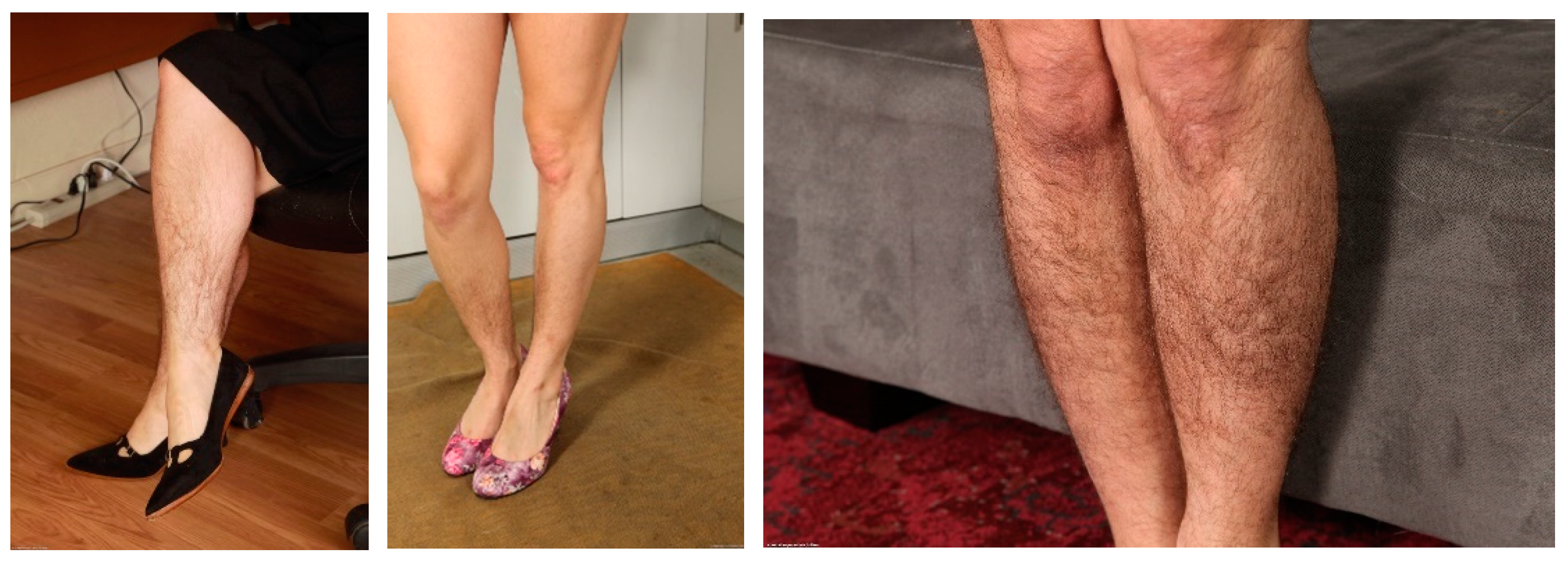
Figure 1. “Leg” images obtained by the data-mining process.
Mathematics 10 03571 g001
Figure 2. Images from the Flickr Image dataset [45].
Mathematics 10 03571 g002
Figure 3. Images of legs with CVD.
Mathematics 10 03571 g003
Figure 4. Images by CEAP classes (the ratio to the total in percent).
Mathematics 10 03571 g004
Figure 5. The Logistic Loss curve for the binary classification model “legs–no legs”.
Mathematics 10 03571 g005
Figure 6. The Logistic Loss curve for the multi-classification model based on Resnet50.
Mathematics 10 03571 g006
Figure 7. The multi-classification model based on Resnet50. The color scheme for confusion matrices (a); the confusion matrices for C0 (b), for C1 (c), and C2 (d) classes.
Mathematics 10 03571 g007aMathematics 10 03571 g007b
Figure 8. The multi-classification model based on Resnet50. The confusion matrices for C3 (a), C4 (b), C5 (c), and C6 (d) classes.
Mathematics 10 03571 g008
Figure 9. The Visual Transformers architecture.
Mathematics 10 03571 g009
Figure 10. The multi-classification model based on vit-base-patch16-224. The confusion matrices for C0 (a), C1 (b), C2 (c), C3 (d), C4 (e), C5 (f), and C6 (g) classes.
Mathematics 10 03571 g010aMathematics 10 03571 g010b
Figure 11. The multi-classification model based on vit-base-patch16-384. The confusion matrices for C0 (a), C1 (b), C2 (c), C3 (d), C4 (e), C5 (f), and C6 (g) classes.
Mathematics 10 03571 g011aMathematics 10 03571 g011b
Figure 12. The Logistic Loss curve for the multi-classification model based on DeiT.
Mathematics 10 03571 g012
Figure 13. The color scheme for confusion matrices for the multi-classification model based on DeiT (a) and the confusion matrices for the C0 class (b).
Mathematics 10 03571 g013
Figure 14. The multi-classification model based on DeiT. The confusion matrices for C1 (a), C2 (b), C3 (c), C4 (d), C5 (e), and C6 (f) classes.
Mathematics 10 03571 g014
Table 1. Training parameters for vit-base-patch16-224 and vit-base-patch16-384.
Parametervit-base-patch16-224vit-base-patch16-384
hidden_size768768
image_size224384
num_hidden_layers1212
patch_size1616
Table 2. The metrics of the different DL models.
NNPrecisionRecallF1 Score
Resnet500.620.610.61
vit-base-patch16-2240.750.750.75
vit-base-patch16-3840.790.790.79
DeiT0.770.770.77
Table 3. The probabilities of classification for each CEAP class.
ModelNNRated TPRated TNRated FPRated FN
C0Resnet500.800.970.200.029
vit-base-patch16-2240.610.980.390.019
vit-base-patch16-3840.710.980.290.015
DeiT0.760.990.240.001
C1Resnet500.790.910.210.086
vit-base-patch16-2240.780.940.220.057
vit-base-patch16-3840.830.960.170.042
DeiT0.860.940.140.055
C2Resnet500.520.900.480.098
vit-base-patch16-2240.670.920.330.082
vit-base-patch16-3840.710.930.290.07
DeiT0.630.950.370.055
C3Resnet500.600.850.400.150
vit-base-patch16-2240.840.890.160.11
vit-base-patch16-3840.850.910.150.087
DeiT0.830.900.170.099
C4Resnet500.470.910.530.085
vit-base-patch16-2240.670.960.330.039
vit-base-patch16-3840.750.960.250.038
DeiT0.700.940.300.058
C5Resnet500.290.910.710.030
vit-base-patch16-2240.60.990.400.009
vit-base-patch16-3840.590.990.410.007
DeiT0.400.990.600.014
C6Resnet500.400.990.600.012
vit-base-patch16-2240.600.990.400.005
vit-base-patch16-3840.791.000.210.004
DeiT0.550.990.450.009
Publisher’s Note: MDPI stays neutral with regard to jurisdictional claims in published maps and institutional affiliations.