Abstract
The current lightweight face recognition models need improvement in terms of floating point operations (FLOPs), parameters, and model size. Motivated by ConvNeXt and MobileFaceNet, a family of lightweight face recognition models known as ConvFaceNeXt is introduced to overcome the shortcomings listed above. ConvFaceNeXt has three main parts, which are the stem, bottleneck, and embedding partitions. Unlike ConvNeXt, which applies the revamped inverted bottleneck dubbed the ConvNeXt block in a large ResNet-50 model, the ConvFaceNeXt family is designed as lightweight models. The enhanced ConvNeXt (ECN) block is proposed as the main building block for ConvFaceNeXt. The ECN block contributes significantly to lowering the FLOP count. In addition to the typical downsampling approach using convolution with a kernel size of three, a patchify strategy utilizing a kernel size of two is also implemented as an alternative for the ConvFaceNeXt family. The purpose of adopting the patchify strategy is to reduce the computational complexity further. Moreover, blocks with the same output dimension in the bottleneck partition are added together for better feature correlation. Based on the experimental results, the proposed ConvFaceNeXt model achieves competitive or even better results when compared with previous lightweight face recognition models, on top of a significantly lower FLOP count, parameters, and model size.
Keywords:
face recognition; face verification; lightweight model; inverted residual block; ConvNeXt block; enhanced ConvNeXt block; ConvFaceNeXt MSC:
68-04; 68T45; 68T10; 68W01
1. Introduction
Face recognition is one of the popular research areas in the field of computer vision. Generally, the common pipelines for face recognition are face detection, face alignment and facial representation for verification or identification. The first step for face recognition is face detection, whereby each person’s face is enclosed with a bounding box [1]. Aside from the frontal face, a robust detector must be able to detect faces across different illuminations, poses and scales [2]. Next, face alignment includes the process of capturing discriminant facial landmarks and aligning the face to normalised canonical coordinates [2]. Normally, alignment transformation is carried out with reference to important facial landmarks such as the eyes’ centre, the nose’s tip and the mouth’s corners. Finally, facial representation is implemented by obtaining the face descriptors from the extracted features. Given a pair of face images, face verification is a one-to-one comparison to determine whether both faces belong to the same person [3]. On the other hand, face identification is a one-to-many comparison in order to match the given unknown face against the known faces in a gallery [4]. If there is a match, then it is considered a closed-set identification; otherwise, it is an open-set identification.
With the recent progress of deep convolutional neural networks, the performance of face recognition systems has been greatly improved. Nevertheless, this comes at the expense of large model sizes and high computational complexity [5,6,7]. In other words, if there are more layers in a convolutional neural network, then the floating-point operations (FLOPs), parameters and model size also tend to be increased. Hence, the employment of the face recognition model in embedded and mobile applications remains a demanding task.
Several efforts have been made to revamp mobile-based networks, which were originally used for generic computer vision applications, to better suit face recognition. These common networks comprise the MobileNet series [8,9] and ShuffleNetV2 [10]. Based on MobileNetV2 [9], a lightweight face recognition model known as MobileFaceNet [11] is introduced. MobileFaceNet adopts the typical inverted residual block design with around 0.47 G FLOPs and 1.03 M parameters. This is followed by ShuffleFaceNet [12], which builds on ShuffleNetV2 [10]. There are four types of architectures with different output channels proposed by ShuffleFaceNet. ShuffleFaceNet has around 0.28 G FLOPs and 1.46 M parameters. Another example is ShuffleFaceNet , which has around 0.58 G FLOPs and 2.70 M parameters. In a more recent publication [13], the authors suggested that ShuffleFaceNet provides a better speed-accuracy trade-off among the four architectures. The MobileFaceNetV1 and ProxylessFaceNAS models [13] were introduced simultaneously by the same authors. With reference to MobileNet(V1) [8], depthwise separable convolution is employed in MobileFaceNetV1 in order to reduce computation. On the other hand, the design of ProxylessFaceNAS has been attributed to the efficient architecture found by the ProxylessNAS [14] network. MobileFaceNetV1 has roughly 1.15 G FLOPs and 3.43 M parameters, while ProxylessFaceNAS possesses 0.87 G FLOPs and 3.01 M parameters.
Lightweight convolutional neural network (LCNN) face recognition models [15] adopt MobileFaceNet [11] as the baseline. Two examples of LCNNs are DSE_LSSE and Distill_DSE_LSSE, both with around 1.35 M parameters. After that, MixFaceNets [16] with six family members is introduced. Motivated by MixNets [17], MixFaceNets utilises depthwise convolution with multiple kernel sizes in the building block. MixFaceNet-S and Shuffle MixFaceNet-S are two of the members, with 0.45 G FLOPs and 3.07 M parameters.
Recently, another model based on inverted residual blocks [9] was introduced, which is known as the efficient, lightweight attention network (ELANet) [18]. The FLOPs and parameter counts for ELANet are 0.55 G and 1.61 M, respectively. At the same time, four face-specific models known generally as PocketNets [19] are designed by utilising the search space of differentiable architecture search (DARTS) [20]. The complexity of these four PocketNets differs in terms of parameters and the output-embedding dimension. For instance, PocketNetS-128 has 0.58 G FLOPs and 0.92 M parameters. Additionally, PocketNetM-128 contains 1.09 G FLOPs and 1.68 M parameters.
Unfortunately, these lightweight face recognition models still suffer from high FLOPs, model sizes and parameters. Motivated by both ConvNeXt [21] and MobileFaceNet [11], a new family of face recognition models termed ConvFaceNeXt is proposed. Note that the key building block of ConvNeXt is known as the ConvNeXt block, while MobileFaceNet deploys an inverted residual block. The structure design of ConvNeXt is based on a large Resnet model, while MobileFaceNet is adapted from lightweight MobileNetV2. Modifications are performed on these two networks so that the proposed ConvFaceNeXt integrates both lower FLOPs and lightweight properties that suit face recognition tasks. Note that FLOPs have an impact on a model’s runtime and computing operations [22]. Generally, for a typical inverted bottleneck block, the depthwise convolution layer is located in between two pointwise convolution layers, which results in increasing FLOPs. Hence, in the revamped inverted bottleneck block, the location of the depthwise convolution layer is moved up to reduce the FLOPs. In addition, the features of each block with the same output dimension are aggregated to generate better facial features. Fewer activation functions and normalisation layers were also found to be beneficial to the overall model performance.
In recent years, lightweight face recognition systems have received increasing interest due to the rapid growth of mobile computing and the Internet of Things (IoT). This trend enables face recognition technology to be adopted by smartphones, embedded systems and wearable devices. As a result, lightweight face recognition technology can be employed in a myriad of mobile applications with limited computational resources. These use cases include user authentication and attendance monitoring as well as augmented reality (AR) and virtual reality (VR) applications for identity verification, to name a few [23,24,25]. For banking and financial services, face recognition is used as an authentication method to verify the identity of a client for online banking using smartphones [26]. In the education sector, face recognition can be implemented on an embedded system for monitoring students’ attendance in a classroom [27]. Pertaining to AR and VR applications in security enforcement, face recognition can be integrated into wearable devices such as Google Glass to help police identify criminals for public safety [28].
Based on the aforementioned factors, the main contributions of this paper can be summarised as follows:
- We propose a family of lightweight face recognition models known generally as ConvFaceNeXt. The proposed models have three major components, namely the stem partition, the bottleneck partition and the embedding partition. With different combinations of downsampling approaches in the stem partition and the bottleneck partition, four models of ConvFaceNeXt are proposed. These downsampling approaches differ in kernel size for convolutional operation. Specifically, the patchify approach involving a non-overlapping patch is introduced in addition to the typical overlapping approach. All of the ConvFaceNeXt models are lightweight yet still able to achieve comparable or better performance.
- We improve and enhance the existing ConvNeXt block for face recognition tasks. Hence, a new structure known as an enhanced ConvNeXt (ECN) block is proposed. Given the same input tensor and expansion factor, the ECN block has significantly lower FLOPs and parameter counts compared with the inverted residual block and ConvNeXt block. These advantages are mainly due to the arrangement of depthwise convolution in the first layer of the ECN block as well as the smaller kernel size. Multiple ECN blocks are stacked repeatedly in the bottleneck partition to form the core part of ConvFaceNeXt.
- We capture more comprehensive and richer face features with less information loss. This is accomplished by aggregating the blocks with the same output dimension for the three respective stages in the bottleneck partition. The aggregation process ensures information correlation for all the generated features within the same stage. In addition, the impact of the vanishing gradient problem can be minimised because the high-level and low-level features of each stage are linked through aggregation. Thus, ConvFaceNeXt models are resistant to information loss, as more feature details can be preserved.
This work provides another alternative form of lightweight model that can be used as a guideline for future vision and face recognition research. The remainder of the paper is organised as follows. In Section 2, the related lightweight face recognition models are reviewed. Section 3 introduces the proposed lightweight face recognition family, which is ConvFaceNeXt. In Section 4, the experimental results of ConvFaceNeXt and other previous lightweight face recognition models are presented and analysed. Finally, Section 5 summarises and concludes this work.
2. Related Works
Several lightweight and efficient face recognition models have recently been proposed for applications with low computational requirements. As a guideline, lightweight face recognition models should have a computation complexity of no more than 1 G of FLOPs, as well as a model size not exceeding 19.8 MB [29]. Most of these lightweight models are based on the modification of the common network architecture used for ImageNet [30] classification. In this section, the related lightweight face recognition models are briefly presented and described as follows:
MobileFaceNet: This model [11] was introduced with the aim of achieving better face recognition accuracy on mobile and embedded applications in real time. Based on MobileNetV2 [9], an inverted residual block is used as the main structure for MobileFaceNet, albeit with a lower reduction factor. In order to reduce the spatial dimension of the raw input face image, convolution with a stride of 2 is used for faster downsampling. In this work, this fast downsampling strategy is denoted as a typical head. Towards the end of the model, global depthwise convolution (GDC) and linear convolution are adopted. GDC is used to reduce the final spatial dimension as well as ensure low computation in the last several convolution layers.
ShuffleFaceNet: With the purpose of accomplishing efficient and accurate performance in face recognition tasks, ShuffleFaceNet [12] models were introduced. ShuffleFaceNet is inspired by ShuffleNetV2 [10], which introduced channel shuffle and channel split units. Both of these units are incorporated into the building block of ShuffleNetV2 for a better flow of information between feature channels. Similar to MobileFaceNet, a typical head is employed at the beginning, while GDC and linear convolution are deployed at the end part of the model. Note that ShuffleFaceNet includes a family of four models, namely ShuffleFaceNet , ShuffleFaceNet , ShuffleFaceNet and ShuffleFaceNet . Each model is scaled with different channel numbers in the block for varying complexities.
MobileFaceNetV1: In order to enhance the discriminative ability of face recognition, MobileFaceNetV1 [13] was developed. Motivated by MobileNet [8], depthwise separable convolution is used as the building block of MobileNetV1 to significantly reduce the computational complexity. Note that depthwise separable convolution is basically the combination of depthwise convolution followed by pointwise convolution. At the beginning of the model, convolution is applied to generate multiple feature maps. Different from MobileFaceNet and ShuffleFaceNet, the first convolution operator of MobileFaceNetV1 is not used for faster downsampling. Instead, the spatial dimension of the input image is retained after the first convolution to preserve more information. Next, several depthwise separable convolutions are stacked sequentially, followed by GDC and linear convolution when approaching the end.
ProxylessFaceNAS: An efficient model known as ProxylessFaceNAS [13] was suggested so that the learned features would be discriminative enough for face recognition tasks.
ProxylessFaceNAS utilizes the CPU model searched by ProxylessNAS [14]. The objective of ProxylessNAS is to learn architecture directly in the target tasks alongside reducing the memory and computational cost. In addition, inverted residual blocks with numerous expansion ratios and kernel sizes are added into the search space of ProxylessNAS. Akin to MobileFaceNetV1, the fast downsampling strategy is not adopted for the first convolution operation. Moreover, inverted residual blocks with larger expansion factors are preferable in the subsequent downsampling operations to avoid losing too much information. After stacking the inverted residual blocks countless times, GDC and linear convolution are performed at the end.
LCNN: A lightweight convolutional neural network (LCNN) [15] is suggested for face recognition with reference to MobileFaceNet [11] as the baseline model. This work investigates the strategies of channelling attention and knowledge distillation towards the performance of the lightweight face recognition model. Specifically, the location of the attention module in an inverted residual block is evaluated in addition to the integration of this module at the end of the model. As a result, three structures based on the squeeze-and-excitation (SE) [31] attention module are introduced, namely depthwise SE (DSE), depthwise separable SE (DSSE) and linear SE (LSE) structures. Based on these structures, various models based on different combinations are constructed. In addition, a larger model based on an improved version of ResNet-50 [32] is used as the teacher model to train the smaller constructed models.
MixFaceNets: Taking computational complexity into consideration, MixFaceNets [16] was developed. The objectives of these models are to reduce the FLOPs and computation overhead. With inspiration from MixNets [17] and ShuffleFaceNet [12], the channels and kernels are mixed up to improve the discriminative capability and performance accuracy. Using depthwise convolution with multiple kernel sizes, MixFaceNets models can obtain resolution patterns at various scales. Similar to ShuffleFaceNet, channel shuffle units are applied to some MixFaceNets models to ensure information flow between channels. In addition, an SE [31] attention module is integrated into the building block of MixFaceNets. There are six family members for MixFaceNets: MixFaceNet-XS, MixFaceNet-S, MixFaceNet-M, ShuffleMixFaceNet-XS, ShuffleMixFaceNet-S and ShuffleMixFaceNet-M. These six models differ in terms of complexity and whether the channel shuffle unit is incorporated.
ELANet: The Efficient Lightweight Attention Networks (ELANet) [18] were introduced with the intention to overcome the challenges of face variations due to changes in pose and age. Motivated by MobileNetV2 [9] and MobileFaceNet [11], the architecture of ELANet consists of multiple inverted residual blocks with a slight modification. Specifically, channel and spatial attention mechanisms are incorporated and applied concurrently in each of the inverted residual blocks, collectively known as the bottleneck attention module. In addition, the multiscale pyramid module is integrated into the architecture to extract and learn features at different scales. Note that a multiscale pyramid module is implemented in every two bottleneck attention modules. The outputs from these multiscale pyramid modules are then united by an adaptively spatial feature fusion module. This is to ensure the comprehensive integration of information in different layers. Finally, all the features are concatenated before the fully connected layer.
PocketNet: Extreme lightweight face recognition models known as PocketNet [19] were developed by utilizing the differential architecture search (DARTS) algorithm [20]. The goal of this work is to search for a family of face-specific lightweight models that can improve face recognition accuracy. Two types of cells are learned by DARTS, namely normal and reduction cells. First, a typical head is implemented for fast downsampling. After that, multiple normal cells and three reduction cells are stacked in series, followed by GDC and linear convolution towards the end. In addition, multi-step knowledge distillation is utilized to transfer knowledge from the large ResNet-100 teacher model to the PocketNet student model. Hence, the performance and generalisation capability of the smaller student model can be improved. Bear in mind that PocketNet is a family with four models: PocketNetS-128, PocketNetS-256, Pocket-NetM-128 and PocketNetM-256. Here, the abbreviations ‘S’ and ‘M’ represent small and medium PocketNet models in terms of parameter counts, respectively. Likewise, ‘128’ and ‘256’ are the output embedding dimensions of the respective models.
LFR: A lightweight face recognition (LFR) model [33] was introduced for embedding devices. The baseline of LFR is adopted from MobileFaceNet [11] with three strategies to optimise the overall model. First, fewer inverted residual blocks are deployed compared with MobileFaceNet in order to have a more efficient model. Second, h-ReLU 6 is used as the activation function for less expensive computing. Essentially, h-ReLu 6 is based on the hard version of the Swish activation function and has an upper bound, which is clipped at six. The final strategy involves applying efficient channel attention (ECA) [34] to the first and last inverted residual blocks. Instead of an SE [31] attention module, ECA is adopted due to its lower memory requirement and computational complexity.
3. Proposed Approach
In this section, the preliminaries of the inverted residual block and ConvNeXt block are reviewed first. Next, the proposed enhanced ConvNeXt (ECN) block is presented, followed by the whole ConvFaceNeXt architecture.
3.1. Preliminaries
Inverted Residual Block: Introduced in MobileNetV2 [9], an inverted residual block is designed for mobile applications. As shown in Figure 1a, the structure of the inverted residual block consists of three convolutional layers. Specifically, first, a pointwise convolution is used to expand the channel dimension. This is then followed by a depthwise convolution to learn the spatial context for each channel and finally another pointwise convolution to reduce the channel dimension. In addition, one batch normalisation and one rectified linear unit (RELU) activation function are applied after each convolution, except for the last convolution, where only one batch normalisation is utilized.
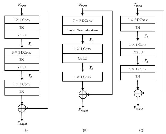
Figure 1.
Different types of building blocks. (a) Inverted residual block. (b) ConvNeXt block. (c) The proposed Enhanced ConvNeXt (ECN) block. Here, ‘Conv’ represents convolution operation, ‘BN’ represents batch normalisation and ‘DConv’ represents depthwise convolution.
Two distinctive characteristics of the inverted residual block are the use of the residual connection between two bottlenecks and the adoption of the linear bottleneck. Note that the residual connection enables the gradient to flow easily across multiple blocks, while the linear bottleneck tends to preserve more information by omitting the activation function of the last pointwise convolution [9]. Due to the light weight and efficiency of the inverted residual block, it is adopted for the face recognition model with low computation and memory requirements. The building block of MobileFaceNet [11] is based on an inverted residual block, albeit with a much smaller expansion factor. ProxylessFaceNAS [13] is modified from the ProxylessNAS network, which adds an inverted residual block as its search space. In addition, ELANet [18] incorporates an attention mechanism in the inverted residual block to prioritise discriminative features.
ConvNeXt Block: ConvNeXt [21] was introduced with the aim to strengthen the importance of the convolutional neural network while still maintaining its efficiency and simplicity. As depicted in Figure 1b, there are three convolutional layers in a ConvNext block. The main difference with inverted residual blocks lies in the position arrangement for those layers. Instead of pointwise convolution, a depthwise convolution is applied to extract spatial information in the first layer. This position arrangement strategy of moving up the depthwise convolution to the first layer helps to reduce the FLOPs significantly, provided that both blocks have the same convolutional kernel size [21]. The remaining structure consists of two pointwise convolutions arranged in sequence. This arrangement enables the channel to be extended first and then reduced subsequently. Aside from that, normalisation and activation functions are applied only once in the ConvNext block. Concretely, layer normalisation is placed after the depthwise convolution, whereas the Gaussian error linear unit (GELU) activation function is located after the first pointwise convolution. Similar to the inverted residual block, there is a residual connection for each ConvNext block.
3.2. Enhanced ConvNeXt Block for the Lightweight Model
The original ConvNeXt block is modified and optimized for lightweight tasks. Here, lightweight is defined as a block with fewer parameters, fewer FLOPs and a smaller size. Hence, the Enhanced ConvNext (ECN) block was designed based on these three perspectives. The building block for ECN is shown in Figure 1c. The ECN block adopts a smaller kernel size for the depthwise convolution such that the parameters, FLOPs and size are reduced.
Moreover, either normalisation or an activation function is applied after each convolutional layer instead of implementing both as in inverted residual block. This in turn helps to reduce the parameter count. Following the works of MobileFaceNet and ShuffleFaceNet, batch normalisation and parametric rectified linear unit (PReLU) activations are adopted in the ECN block in lieu of layer normalisation and GELU in the ConvNeXt block. Moreover, as observed from the experiment, the performance of layer normalisation is poor compared with batch normalisation for the ECN block. Let and denote the input and output tensors for an ECN block, respectively. Assuming that the input and output of the ECN block have the same spatial and channel dimension, here, H, W and C are those tensors’ height, width and number of channels, respectively.
The first part consists of implementing a depthwise convolution followed by a batch normalisation operation. Note that the stride s of depthwise convolution is set to one for a block with the same input and output dimensions. In the second part, a pointwise convolution with an expansion factor t is utilized for channel expansion before appending a PReLU activation function. Next, one more pointwise convolution is employed for channel reduction prior to batch normalisation. Finally, a residual connection is used to connect both input and output tensors. The whole process of the ECN block can be mathematically represented as follows:
where and correspond to the depthwise and ith pointwise convolution, b is the batch normalisation operation, a indicates the PReLU activation function and and represent the intermediate features obtained from the first and second parts, respectively. In summary, the overall workflow of the ECN block is given in Table 1.

Table 1.
The workflow of the ECN block. Here, ‘DConv’ denotes depthwise convolution, ‘Conv’ denotes convolution operation and ‘BN’ denotes batch normalisation.
3.3. ConvFaceNeXt Architecture
Motivated by ConvNeXt and MobileFaceNet, a family of four novel lightweight face recognition models known generally as ConvFaceNeXt were proposed. The ConvFaceNeXt models consist of three major components, namely the stem partition, the bottleneck partition and the embedding partition. The core architecture for ConvFeaceNeXt models is formed by stacking multiple ECN blocks sequentially in the bottleneck partition. In addition, numerous downsampling approaches are combined in the stem partition and bottleneck partition, which results in four different sets of architecture design for ConvFaceNeXt family members. Given a face image in the stem partition, the stem cell is utilized to downsample the spatial dimension by half as well as generate 64 output channels. The stem cell operator can either be a or a convolution, both with a stride of two. The first option is known as patchify head (PH), inspired by ConvNeXt, while the second is the typical head (TH), used by previous lightweight face recognition models. Both operators involve a stride of two.
Depthwise separable convolution is performed afterwards to encode spatial and inter-channel information. For the bottleneck partition, the downsampling and ECA blocks are stacked together in several stages. There are two designs for the spatial downsampling block. Motivated by ConvNeXt, the first involves a separate downsampling (SD) block of a convolution with a stride of two. The second alternative, which is designated the ECN downsampling (ED) block, utilizes a depthwise convolution with a stride of two in the ECN block, where the residual connection is removed. Notably, these downsampling and ECN blocks are arranged with a stage computing ratio of 5:8:3 in ConvFaceNeXt.
Bear in mind that the stride is set to two for those downsampling blocks. Otherwise, it is fixed to one for the remaining blocks in the same stage. Moreover, the outputs of all the blocks in the same stage are linked together. Specifically, all of the outputs are summed so that the low-level and high-level face features can be correlated effectively. This is inspired by the linking strategy adopted by EEPNet [35] to avoid blurriness in the palm print feature. In the subsequent embedding partition, a convolution followed by a linear global depthwise convolution is performed. Finally, a linear convolution is employed to obtain a compact 128-dimension vector embedding for each face image. In contrast to the conventional technique of applying both batch normalisation and activation functions after each convolution, ConvFaceNeXt adopts either one. Hence, the overall architecture is lightweight yet with comparable or better performance.
In order to gain a better understanding and ensure clarity, Table 2 presents the general settings for each of the four ConvFaceNeXt architecture designs. Specifically, ConvFaceNeXt, which employs a patchify head and separate downsampling block, is known as ConvFaceNeXt_PS. In addition, ConvFaceNeXt with a patchify head and ECN downsampling block is addressed as ConvFaceNeXt_PE. The subsequent model deploys a typical head along with a separate downsampling block, termed as ConvFaceNeXt_TS. Finally, the last model combines both a typical head and ECN downsampling blocks, dubbed ConvFaceNeXt_TE. The following subsections describe in detail each of the three partitions in ConvFaceNeXt based on the graphical and tabulated outlines, as illustrated in Figure 2 and Table 3, respectively.
Table 2.
The general architecture design for each ConvFaceNeXt family member.
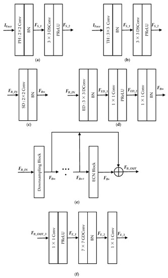
Figure 2.
Graphical outline of the proposed ConvFaceNeXt model. (a) Stem partition with the patchify head configuration. (b) Stem partition with typical head configuration. (c) Bottleneck partition with separate downsampling configuration. (d) Bottleneck partition with ECN downsampling configuration. (e) Linking of blocks with same output dimension for a particular stage in bottleneck partition. (f) Embedding partition. Here, ‘PH’ refers to the patchify head, ‘TH’ refers to the typical head, DSConv denotes depthwise separable convolution, ‘SD’ refers to separate downsampling, ‘ED’ refers to ECN downsampling and ‘GDConv’ denotes global depthwise convolution.
Table 3.
Tabulated outline of the proposed ConvFaceNeXt model. Each row denotes a sequence of operators. Here, t denotes the expansion factor for downsampling and ECN blocks. Note that for the downsampling block, the expansion factor only applies to the ED block (shown with *), while there is none for the SD block. In addition, a stride s of two is set for all the downsampling blocks, while the other ECN blocks use a stride of one.
3.3.1. Stem Partition
At the beginning of the model, stem partition is used to downsample and extract raw information from the input face image. Hence, ConvFaceNeXt uses a patchify head (PH) or typical head (TH) to process the input image into a proper feature size. For PH, the input image is split into non-overlapping patches according to the size of the convolution kernel. Unlike ConvNeXt, which adopts a convolution and a stride of 4, the PH of ConvFaceNeXt uses a convolution and a stride of two due to a smaller input image size. On the other hand, a TH is implemented through a convolution with a stride of two. This is similar to the approach used in MobileFaceNet, ShuffleFaceNet and PocketNet. In addition, batch normalisation is appended to the stem cell. After that, a depthwise separable convolution followed by a PReLU activation function is performed to encode useful spatial and channel information. The whole process for stem partition is shown in Figure 2a,b.
Supposing that is the input face image, the first stem feature and the second stem feature outputs from the respective convolution and depthwise separable convolution can be mathematically formulated as follows:
and
where refers to the convolution operation f with a kernel size m. Note that m is for ConvFaceNeXt with a PH ( ConvFaceNeXt_PS and ConvFaceNeXt_PE) and for ConvFaceNeXt with a TH (ConvFaceNeXt_TS and ConvFaceNeXt_TE). Aside from that, represents the depthwise separable convolution. This way, richer information can be extracted by appending two convolution layers.
3.3.2. Bottleneck Partition
The bottleneck partition is the most important part of the entire model. Utilizing ECN blocks, the bottleneck partition enables the total FLOPs of the model to be reduced as a whole. That aside, the outputs of all the downsampling and ECN blocks in a particular stage are aggregated with the aim of having better correlation among different features. This in turn will help prevent the vanishing gradient problem and lessen information loss. There are three main stages in the bottleneck partition, where the number of blocks in each stage is five, eight and three, respectively. Figure 2c–e illustrates the operating procedures of the bottleneck partition. From the bottleneck partition in Table 3, each stage starts with a downsampling block, whereas the remaining are ECN blocks.
In order to reduce the spatial dimension, ConvFaceNeXt adopts either separate downsampling (SD) or an ECN downsampling (ED) approach. SD is considered more aggressive and faster than ED. The reason for this is that only one convolution operation is performed in SD, while there are three convolution operations for ED. Concretely, two ConvFaceNeXt models employ an SD block (ConvFaceNeXt_TS and ConvFaceNeXt_PS), whereas the remaining two adopt an ED block (ConvFaceNeXt_PE and ConvFaceNeXt_TE). As illustrated in Figure 2c, is the input for a particular stage in the bottleneck partition, and then the output of the SD block is
where denotes the convolution operation. Using the same input and output notations of the SD block, the following equations show the output for the ED block in series as depicted in Figure 2d:
where and are the intermediate features generated by the depthwise convolution and first pointwise convolution, respectively.
In an ECN block, information is obtained sequentially through feature extraction using depthwise convolution, feature expansion using pointwise convolution, and feature compression using another pointwise convolution. Different from the larger depthwise convolution used in the ConvNeXt block, ConvFaceNeXT employs a depthwise convolution in the ECN block, which is a better option for face recognition tasks. Generally, there is a residual connection to link the input and output of the ECN block with the same dimension. Referring to the bottleneck partition in Table 3, we note that ConvFaceNeXt has no residual connection for ECN blocks 7 and 15 in stages 2 and 3, respectively. In order to further improve the performance while maintaining a low FLOP count, the output from downsampling and the ECN blocks in the same stage are aggregated together. Hence, the aggregated output feature shown in Figure 2e can be generally expressed as
where is the output of the jth block while m and n represent the first and last index of a block in a particular stage, respectively. To be precise, the block indices for each stage are 1–5 for stage 1, 6–13 for stage 2 and 14–16 for stage 3. Here, blocks 1, 6 and 14 are the downsampling blocks, and the others are ECN blocks.
3.3.3. Embedding Partition
This partition is used to obtain the face embedding. All the ConvFaceNeXt models employ the same setting in the embedding partition. Different from ConvNeXt, global average pooling and fully connected layers are not employed. This is because global average pooling is less accurate for face verification, while fully connected layers consume a huge amount of parameters [11]. The increase in parameters leads to a larger model size, which essentially deviates from ConvFaceNeXt’s purpose of introducing a lightweight face recognition model. First, the features are increased using a convolution along with the PReLU activation function. Then, the spatial dimension is reduced with a linear global depthwise convolution followed by batch normalisation. Eventually, the face embedding with a 128-dimension vector is obtained via a linear convolution.
Previous works adopted the same three convolution operators to extract face embedding. However, the approach of ConvFaceNeXt is slightly different in terms of deploying fewer batch normalisation operations. The entire process of the embedding partition is depicted in Figure 2f. Let and denote the output features of the first, second and third convolutions in the embedding partition, respectively. Then, the aforementioned steps can be mathematically formulated as
where is the output feature from the last stage of the bottleneck partition and is the global depthwise convolution.
4. Experiments and Analysis
In this section, the training and evaluation datasets for all of the ConvFaceNeXt family and previous lightweight face recognition models are presented first. After that, the experimental settings for all these models are described. This is followed by ablation studies to determine the same effective design scheme for all the ConvFaceNeXt models. Then, quantitative analysis is conducted based on the verification accuracy of the evaluation dataset for all the models. Finally, qualitative analysis involves the assessment of images by visual observation.
4.1. Dataset
UMD Faces [36] was employed as the training dataset for all the models. This is a medium-sized dataset consisting of 367,888 face images for 8277 individuals. The reason for choosing this dataset was because it has more pose variations compared with other similar-sized datasets, such as CASIA WebFace [37] and VGGFace [38]. Note that CASIA WebFace comprises 494,414 images of 10,575 individuals, while VGGFace has 2.6 million images from 2622 individuals. During the training of ConvFaceNeXt, the dimensional face images were detected and aligned through multi-task cascaded convolutional networks (MTCNN) [39] were obtained from the face.evoLVe library [40]. In order to evaluate the efficiency of ConvFaceNeXt, seven image-based and two template-based datasets with various aspects were used as evaluation benchmarks. These datasets are listed below:
- The Labeled Faces in the Wild (LFW) [41] dataset consists of 13,233 face images from 5749 identities. The majority of the face images are frontal or near-frontal. The verification evaluation comprises 6000 pairs of face images, which includes 3000 positive face pairs and 3000 negative face pairs.
- Cross-Age LFW (CALFW) [42] is the revised version of LFW, where 3000 positive face pairs are obtained from the same individual with a notable age gap, whereas the remaining 3000 negative face pairs are from different individuals of the same gender and race.
- Cross-Pose LFW (CPLFW) [43] is derived from LFW with intra-class pose variation for the 3000 positive face pairs while ensuring the same gender and race attributes for the other 3000 negative face pairs.
- The CFP [44] dataset contains 7000 face images from 500 identities, where each identity has 10 frontal and 4 profile face images. There are 3500 positive face pairs and 3500 negative face pairs. The evaluations are conducted based on two protocols, namely frontal-frontal (CFP-FF) and frontal-profile (CFP-FP).
- AgeDB [45] includes 16,488 face images of 568 identities used for age-invariant face verification. This dataset contains 3000 positive and 3000 negative face pairs. There are four face verification protocols, each with different age gaps of 5, 10, 20 and 30. AgeDB-30, with the largest age gap, was used for evaluation since it is harder compared with the other three protocols.
- VGGFace2 [7] comprises 3.31 million face images from 9131 individuals. The VGGFace2 dataset is split into two parts, where the training dataset has 8631 individuals while the evaluation set has only 500 individuals. Two evaluation protocols are available, which include evaluation over the pose and age variations. VGG2-FP, which emphasizes pose variation, was chosen as the benchmark to evaluate 2500 positive and 2500 negative face pairs.
- IARPA Janus Benchmarks (IJB) [46,47] set a new phase in unconstrained face recognition with several series of datasets. These datasets are more challenging, with further unconstrained face samples under significant pose, illumination and image quality variations. In contrast to other image-to-image or video-to-video datasets, each IJB is a template-based dataset with both still images and video frames. The IJB-B [46] dataset consists of 1845 individuals. This dataset has 21,798 still images in addition to 55,026 frames from 7011 videos. The 1:1 baseline verification of the IJB-B dataset is based on 10,270 genuine comparisons and 8 million imposter comparisons. On the other hand, there are 3531 individuals for the IJB-C [47] dataset. This dataset comprises 31,334 still images alongside 117,542 frames from 11,779 videos. The 1:1 baseline verification consists of 19,557 genuine comparisons and 15,638,932 imposter comparisons.
The evaluation metrics for the aforementioned testing dataset were conducted based on the verification tasks. For LFW, CALFW, CPLFW, CFP-FF, CFP-FP, AgeDB-30 and VGG2-FP, the evaluation metric for face pairs is verification accuracy. The performance of the IJB-B and IJB-C datasets were evaluated in terms of the true accept rates (TARs) at false accept rates (FARs) of 0.001, 0.0001 and 0.00001.
4.2. Experimental Settings
All of the models were implemented using the TensorFlow platform. These models were trained from scratch using a stochastic gradient descent optimizer. The momentum and weight decay were set to 0.9 and 0.0005, respectively. In addition, a cosine learning schedule was employed with an initial value of 0.1 and decreased factor of 0.5. Due to GPU memory limitations, these models were trained with a batch size of 256 for 49 epochs. The training was conducted on an NVIDIA Tesla P100 GPU. In addition, ArcFace [32] was adopted as the loss function L for all of these models. The purpose of the loss function is to increase the inter-class differences and reduce the intra-class variations. Specifically, ArcFace tends to increase the discriminative power of learned face features through the additive angular margin m. Hence, the formulation for ArcFace to predict the probability of feature belonging to identity class is given as
where N is the batch size, C is the total number of classes in the training dataset, h is the scaling hyperparameter and is the angle between the feature and the ith class centre.
4.3. Ablation Studies
In this section, several experiments are implemented to analyse the impacts of various settings in ConvFaceNeXt with respect to the final results, FLOPs and parameters. Based on the hill climbing technique [48], these experiments can be categorized into three main parts to tune and determine the best-performing design architecture for ConvFaceNeXt. The overview of these experiments is depicted in Figure 3. Note that ConvFaceNeXt_PE is used as the reference model to carry out all the experiments in ablation studies, as all four family models utilise the same ECN core structure. First, the effect of linking ECN blocks in different stages is investigated. Second, the influence of different kernel sizes on the depthwise convolution in the ECN block is studied. Finally, the amount of batch normalisations and activation functions in the ECN block is investigated. The final results for all the experiments are reported for the image-based datasets (LFW, CALFW, CPLFW, CFP-FF, CFP-FP, AgeDB-30 and VGG2-FP) and template-based datasets (IJB-B and IJB-C).
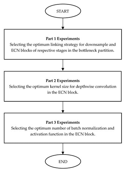
Figure 3.
Flow chart depicting experiments conducted based on hill climbing technique to tune and determine optimum architecture for ConvFaceNext.
4.3.1. Effect of Different Linking Strategies
In order to gain insight into the optimum linking strategy for all the downsampling and ECN blocks in the three respective stages of the bottleneck partition, three experiments were conducted. Note that the linkage was implemented through aggregating the output feature of the downsampling and ECN blocks with the same output dimension. The first model was built with no feature aggregation. The second model only aggregated the output features of the blocks in the first stage. In contrast, the third model considered the aggregating features of the blocks in the first two stages. The last model connected all the blocks with the same output dimension for the three respective stages.
The experimental results for each model are shown in Table 4 and Table 5 and Figure 4. It can be observed that the model with aggregation at all stages had the best overall performance for most evaluation datasets compared with the other three models. Aside from that, the performance gain was achieved without having to incur any additional parameters or FLOPs. This was due to better correlation among the multiple features implemented through aggregating features with the same output dimension for all three stages.
Table 4.
Performance results of the different linking strategies. These results are reported in terms of parameters, FLOPs and verification accuracy for LFW, CALFW, CPLFW, CFP-FF, CFP-FP, AgeDB-30 and VGG-2FP. Aside from that, the average accuracy for the seven image-based datasets is shown in the last column. Here, ‘0A’ denotes no aggregation for all the stages in the bottleneck partition, ‘1A’ denotes aggregation in stage 1, ‘2A’ denotes aggregation in the first two stages (stage 1 and 2), and the last row represents the model with aggregation for all the stages.
Table 5.
Verification accuracy of different linking strategies on IJB-B and IJB-C datasets.
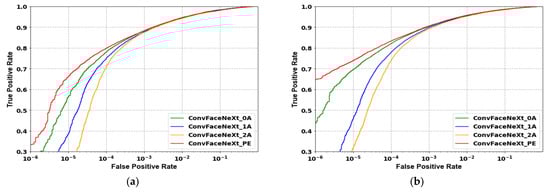
Figure 4.
ROC curves of 1:1 verification for different linking strategies. (a) IJB-B dataset. (b) IJB-C dataset.
In addition, the vanishing gradient problem can be reduced, retaining more face feature information. Normally, this problem occurs when the gradient of the loss function becomes too small during backpropagation. Hence, the weights of the model cannot be updated effectively, leading to information loss and poor performance. From the results, it is noted that the model with aggregation in stage one (ConvFaceNeXt_1A) had a comparable result to the model without aggregation (ConvFaceNeXt_0A) for those seven image-based datasets. The reason for this might be the model with aggregation in stage one only linking lower-level features such as edges and simple textures without considering the correlation of higher-level features in stages two and three, which contained more face details.
It is also interesting to observe that the model with aggregation in stage one as well as the model with aggregation in stages one and two (ConvFaceNeXt_2A) had lower performance in the template-based dataset compared with the model with no aggregation. This is because both models only linked features in certain stages and did not fully utilise the correlation between multi-level features in different stages. Without feature aggregation in the following stage, the correlated information learned in the previous stage could not be forwarded effectively. This proves that it is crucial to aggregate features with the same output dimension for all three stages for extensive and richer feature representation.
4.3.2. Effect of Different Kernel Sizes
In this section, experiments are conducted to determine the optimum kernel size for depthwise convolution of the ECN block. These kernel sizes included three, five, seven and nine. The results of applying various kernel sizes are shown in Table 6 and Table 7 and Figure 5. These results conform to the fact that a larger kernel size does lead to better performance, as in the case of increasing the kernel size from 3 to 5 for the seven image-based datasets.
Table 6.
Performance results of different kernel sizes. These results are reported in terms of parameters, FLOPs and verification accuracy for LFW, CALFW, CPLFW, CFP-FF, CFP-FP, AgeDB-30 and VGG-2FP. That aside, the average accuracy for the seven image-based datasets is shown in the last column. Here, the first row represents a model with a kernel size of three in the depthwise convolution of the ECN block, ‘5K’ refers to a kernel size of five, ‘7K’ refers to a kernel size of 7, and ‘9K’ refers to kernel size of nine.
Table 7.
Verification accuracy of different kernel sizes on IJB-B and IJB-C datasets.
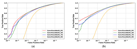
Figure 5.
ROC curves of 1:1 verification for different kernel sizes. (a) IJB-B dataset. (b) IJB-C dataset.
However, there was a limitation wherein the performance tended to saturate beyond a kernel size of five. Note that ConvNeXt employed a kernel size of seven for the depthwise convolution to increase performance. However, from the conducted experiments, it was observed that a larger kernel size resulted in less desirable performance for face recognition tasks, especially for the and kernel sizes. This may be attributed to the input image size of ConvNeXt being , while it was only for ConvFaceNeXt. Hence, the local information extracted by a larger kernel size will be substantially less than for a smaller kernel size.
Although there was an increase in performance for the model with a kernel size of five in most of the aforementioned image-based datasets, this came at the cost of additional computation. Therefore, the parameters and FLOPs increased by about 2.5% and 3.6%, respectively, when the kernel size was switched from three to five. In addition, the model with a kernel size of three performed better as a whole in the IJB-B and IJB-C datasets. A possible reason might be that a smaller kernel size can extract more detail and the minute features of unconstrained face templates in the IJB dataset. Based on the reasons above and the aim to propose a lightweight face recognition model, ConvFaceNeXt adopted a depthwise convolution in each ECN block.
4.3.3. Effect on Different Numbers of Batch Normalisations and Activation Functions
In a typical inverted residual block, each convolution is followed by one batch normalisation and one activation function, with the exception of the last convolution, which is appended with one batch normalisation. As a result, three batch normalisations and two activation functions are utilized in an inverted residual block. In contrast, the ConvNeXt block normalizes the output of the first convolution layer and applies the activation function on the second convolution layer. Hence, normalisation and activation are only used once in the ConvNeXt block. These concepts were adapted to examine the suitable amount of batch normalisations and activation functions in an ECN block for better performance. Specifically, the first model adopts the ConvNeXt strategy with one batch normalisation and PReLU activation in the ECN block, as shown in Figure 6a. The second model contains two batch normalisations and one PReLU activation function in the ECN block, as depicted in Figure 1c. The last model follows the inverted residual block approach, comprising three batch normalisations and two PReLU activation functions, as illustrated in Figure 6b.
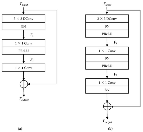
Figure 6.
Building blocks with different amounts of batch normalisations and activation functions. (a) ECN block with one batch normalisation and one PReLU activation. (b) ECN block with three batch normalisations and two PReLU activations.
From the results in Table 8 and Table 9 and Figure 7, the first model with one batch normalisation and one activation function had the smallest parameter and FLOP counts, albeit with inferior performance in the image-based dataset compared with the other two models. For the second model with two batch normalisations and one activation function, the parameter count minimally increased by 0.66% while maintaining the same amount of FLOPs as the first model. In addition, competitive performance was observed in the second model for all the evaluation datasets compared with the first and last models. It was observed that the last model with three batch normalisations and two activation functions showed comparable or slightly better performance. Nevertheless, there were 2.2% and 0.23% increments for the parameter and FLOP counts with respect to the lightest first model.
Table 8.
Performance results for different amounts of batch normalisations and activation functions. These results are reported in terms of parameters, FLOPs and verification accuracy for LFW, CALFW, CPLFW, CFP-FF, CFP-FP, AgeDB-30 and VGG-2FP. Aside from that, the average accuracy for the seven image-based datasets is shown in the last column. Here, ‘1B1P’ denotes the ECN block with one batch normalisation and one PReLU activation, the model in the second row utilizes two batch normalisations and one activation function in the ECN block, and ‘3B2P’ denotes three batch normalisations and two PReLU activations.
Table 9.
Verification accuracy of different amounts of batch normalization and activation functions on IJB-B and IJB-C datasets.
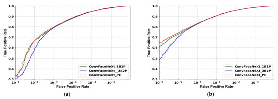
Figure 7.
ROC curves of 1:1 verification on different amounts of batch normalisations and activation functions. (a) IJB-B dataset. (b) IJB-C dataset.
Moreover, more batch normalisations and activation functions tended to slow down the training [49]. Note that the strategy of one batch normalisation and one activation function in the ConvNeXt block is recommended for the ImageNet [30] classification task. Nonetheless, the approach of using two batch normalisations and one activation function in an ECN block is more suitable for face recognition tasks. This is evidenced by the experimental results as well as balancing out the computation complexity and performance.
4.4. Quantitative Analysis
In this section, the experimental results for all lightweight face recognition models are reported. Based on the ablation studies in Section 4.3, the family of four ConvFaceNeXt models followed the same settings, which were aggregating features in the three respective stages, adopting a depthwise convolution as well as utilizing two batch normalisations and one activation function in an ECN block. Moreover, other models such as MobileFaceNet, the ShuffleFaceNet series, MobileFaceNetV1 and ProxylessFaceNAS were compared with the ConvFaceNeXt family. Generally, comparisons between models tend to be biased due to the deployment of different training and testing datasets. In order to be fair, the results are presented with all the aforementioned models trained from scratch using the UMD face dataset. In addition, all the models were trained using the same experiment settings, as discussed in Section 4.2. These models were evaluated on the LFW, CALFW, CPLFW, CFP-FF, CFP-FP, AgeDB-30, VGG2-FP, IJB-B and IJB-C datasets. The results are shown in Table 10 and Table 11.
Table 10.
Performance results of different models. These results are reported in terms of parameters, FLOPs, model size and verification accuracy for LFW, CALFW, CPLFW, CFP-FF, CFP-FP, AgeDB-30 and VGG-2FP. Aside from that, the average accuracy for the seven image-based datasets is shown in the last column.
Table 11.
Verification accuracy of different models on IJB-B and IJB-C datasets.
For the first part, the results for the four models from the ConvFaceNeXt family were compared. Using the average accuracy, the overall performance of ConvFaceNeXt_TE was the best (92.55%) for the image-based datasets. In contrast, with a slight difference of 0.26%, ConvFaceNeXt_PE achieve the lowest average accuracy (92.29%) among the four models. However, this low accuracy is still competitive or better than the other previous lightweight face recognition models.
From our observations, the models with the same stem and bottleneck downsampling strategies were better than the mixed combinations. For example, ConvFaceNeXt_TE utilizes a convolution while ConvFaceNeXt_PS deploys a convolution for both stem and bottleneck downsampling. Hence, information can be transferred in a more coherent and systematic way from low-level to high-level feature maps. Another possible reason for the high accuracy in ConvFaceNeXt_TE is that more features can be extracted due to the larger number of parameters and FLOPs.
In terms of the computational aspect, ConvFaceNeXt_PS and ConvFaceNeXt_TS were more efficient. This was because both models employed the SD downsampling block, which has only one convolution layer, reducing the parameter and FLOP counts compared with the models that adopt the ED block with three convolutions. On the whole, ConvFaceNeXt_PS was the most efficient and lightweight model among the family members, with only 0.96 M parameters, 390.13 M FLOPs and a 4.11-MB model size, yet it was still able to achieve an average accuracy of 92.52%, which is considered high.
For the template-based IJB dataset, ConvFaceNeXt_TS and ConvFaceNeXt_TE had better performance among the ConvFaceNeXt family. The similarity between these two models is that both utilise the typical head to downsample the raw input image. The likely cause may be that the typical head uses a convolution with a stride of two. Therefore, as the kernel slid across the input image, there was an overlapping region among the current and previous kernel cells to ensure information continuity. However, this interrelationship did not exist for the patchify head, where the image was split into non-overlapping patches, thus resulting in raw information loss.
In the second part, the performance of the ConvFaceNext family and the other lightweight face recognition models was compared. Among the previous works, MobileFaceNet had the highest average accuracy at 92.27%. In comparison with the proposed family members, ConvFaceNeXt_PE was 0.02% better than MobileFaceNet at the lower end, whereas ConvFaceNeXt_TE was 0.28% better at the higher end. On top of that, the main advantages of ConvFaceNeXt family members were having fewer parameters and lower FLOP counts. This was especially true for ConvFaceNeXt_PS, which had 6.3% fewer parameters and 17.5% fewer FLOPs than MobileFaceNet but still outperformed MobileFaceNet for almost all evaluation datasets, except for AgeDB-30.
Note that the parameter and FLOP counts of ConvFaceNeXt_PS were also the lowest among all the models. In addition, ConvFaceNeXt_PS surpassed all models on the LFW, CPLFW and VGG2-FP datasets. Other family members also showed significant performance, wherein ConvFaceNeXt_TE recorded the highest accuracy in the CFP-FF dataset while ConvFaceNeXt_TS did so in the CFP-FP dataset. For the remaining AgeDB-30 and CALFW datasets, the optimal performance was attained by MobileFaceNet and MobileFaceNetV1, respectively. On the IJB unconstrained face dataset, the ConvFaceNeXt family yield better performance in general, and specifically, ConvFaceNeXt_TS outperformed other previous models.
These observations indicate that ConvFaceNext models perform well in frontal and cross-pose datasets but are slightly less than optimal for cross-age face images. A possible explanation for the deterioration in the cross-age dataset is that the depthwise convolution for spatial processing in the ECN block has fewer channels than the inverted residual block. Therefore, there will be less information for age-invariant feature extraction. As a complement to Table 10, the published LFW results for previous models, along with the training dataset and loss function, are shown in Table 12.
Table 12.
Verification accuracy on LFW dataset, as published in the works of previous lightweight face recognition models. The stated accuracy was obtained from the respective published paper, whereby each model was trained with a different dataset and loss function.
Note that CosFace [50] was used as the loss function for both MobileFaceNet V1 and ProxylessFaceNAS, as the authors found that ArcFace [32] had lower verification accuracy for both of these models [13]. It is noted that the LFW accuracy for MobileFaceNet increased from 99.28% to 99.55% when employing the Cleaned MS-Celeb-1M dataset, which has more face images than the CASIA dataset. Hence, it is unfair to compare them directly with the published results since a larger dataset yields better performance.
Although the proposed ConvFace NeXt_PS model was trained with the least face images, due to computation constraints, the accuracy was 99.30%, which was better than the models trained with larger datasets such as MobileFaceNet with CASIA at 99.28% and ProxylessFaceNAS with MS1M_RetinaFace at 99.20%. For the LCNN models, a distillation of knowledge from a larger model indeed improved the performance of the smaller model, as observed in the comparison between LCNN (DSE_LSE) and LCNN (Distill_DSE_LSE). Moreover, the accuracy for the LCNN (Distill_DSE_LSE) model was relatively high at 99.67% because both the channel attention and knowledge distillation strategies were deployed to improve the performance. Following the reported results of the MixFaceNets models, which were arranged according to the number of FLOPs, only MixFaceNet-S and ShuffleMixFaceNet-S were taken into account. These two MixFaceNets models had similar computational complexities to the ConvFaceNeXt family members. Although the accuracies were higher for these two MixFaceNets models by around 0.3% to 0.6%, the parameter counts were three times higher than those of the ConvFaceNeXt models.
In more recent works, ELANet achieved the best LFW accuracy at 99.68%. Compared with the proposed ConvFaceNeXt_PS, which reduced the parameter and FLOP counts by about 40% and 30%, respectively, there was only a 0.4% drop in the LFW accuracy. Moreover, unlike ELANet, which utilizes channel and spatial attention to boost performance, the proposed model is purely a lightweight face recognition model without any attention strategy. PocketNet is another contemporary lightweight face recognition model with four family members. In line with the other models in Table 12, which had 128-dimension output embedding, only PocketNetS-128 and PocketNetM-128 were considered. For models with less than 1 M parameters, the LFW accuracy for Pocket-NetS-128 and ConvFace NeXt_PS was 99.58% and 99.30%, respectively. Although the accuracy decreased by 0.28%, ConvFace NeXt_PS had comparable parameters and 30% fewer FLOPs than PocketNetS-128.
On the other hand, for the models with over 1 M parameters, the LFW accuracy for PocketNetM-128 was 99.65%, while ConvFace NeXt_PE achieved an accuracy of 99.10%. Even though there was an accuracy drop of 0.55%, ConvFace NeXt_PE had 37% fewer parameters and 63% fewer FLOPs than PocketNetM-128. In order to further boost performance, a multi-step knowledge distillation strategy was deployed to transfer the knowledge from a large ResNet-100 model to the smaller PocketNet models. With MobileFaceNet as the baseline, the accuracy for LFR was lower, being 98.52%. This might be due to the fewer inverted residual blocks in LFR. Compared with the other remaining models, the proposed ConvFaceNeXt family members achieved competitive accuracies, since the other models were trained with 10 times more face images. Therefore, it is expected that the performance for the proposed ConvFaceNeXt models can be improved by using a larger training dataset as well as utilizing additional strategies.
4.5. Qualitative Analysis
In order to show the effectiveness of the proposed ConvFaceNeXt family members in recognizing and localizing important face features, random examples of positive face image pairs were illustrated using the Grad-CAM [51] technique. These pairs were taken from various conditions, namely frontal, cross-pose and cross-age face image pairs, to show the generalisation of the proposed methods in different aspects. Note that the two face images in each pair corresponded to the same individual. The frontal image pairs were taken from LFW, the cross-pose images were from CPLFW, and the cross-age images were from the CALFW dataset. The visualisation included all four proposed ConvFaceNeXt members and five previous lightweight face recognition models trained under the same dataset and settings. Note that the architecture of all nine methods consisted of a pure convolutional neural network structure without deploying any additional attention mechanism.
Two face image pairs from LFW are shown in Figure 8. For the first pair, the upper image shows a lady wearing a hat with a near-frontal face position, while the bottom image is the corresponding frontal face image without a hat. In the Grad-CAM visualisation, the importance of a feature is highlighted with a colour scale. Specifically, the red region refers to the most important part, followed by the green region and finally the blue region, which is the least important part. Generally, it was observed that the proposed ConvFaceNeXt family members were able to emphasise the face region compared with the previous models. For the face image with a hat, ConvFaceNeXt_TE showed the strongest excitation on the eye and nose parts, highlighted in the orange and yellow regions, respectively. Hence, discriminative face parts can be emphasized. Note that discriminative face parts such as the eyes, nose, mouth and ears are crucial for face recognition tasks [52]. Other previous models showed less desirable outcomes. MobileFaceNet is only able to highlight the left region of the face, with no emphasis given to the discriminative face parts. A similar situation was observed in ShuffleFaceNet , with excitation only on the forehead. Although both ShuffleFaceNet 1.5× and ProxylessFaceNAS could highlight the face region, other unnecessary areas were mainly excited, which are also indicated by the orange and yellow background areas.
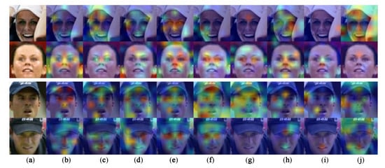
Figure 8.
Two random face image pairs from the LFW dataset. The original image pairs are shown in (a), and the corresponding Grad-CAM visualisations for ConvFaceNeXt family members are illustrated from (b) to (e), while those for the other previous works are shown from (f) to (j), with all arranged column-wise from left to right. (a) Original face image pairs. (b) ConvFaceNeXt_PS. (c) ConvFaceNeXt_PE. (d) ConvFaceNeXt_TS. (e) ConvFaceNeXt_TE. (f) MobileFaceNet [11]. (g) ShuffleFaceNet [12]. (h) ShuffleFaceNet [12]. (i) MobileFaceNetV1 [13]. (j) ProxylessFaceNAS [13].
In contrast, the MobileFaceNetV1 highlighted area does not belong to a face, shown as the orange region in the bottom right. For the frontal face image of the lady without a hat, ConvFaceNeXt_PS and ConvFaceNeXt_TE had the most significant response in the eye, nose and ear regions. Other methods could also highlight the face region to a certain extent, except for ProxylessFaceNAS, where only the forehead was emphasized. The second face pair showed a man wearing a hat for both frontal face images. From our observation, it was noticed that the ConvFaceNeXt family members had the capability to locate discriminative face parts. On the other hand, some previous models tended to highlight the background too or areas with no excitation at all.
Another two pairs of cross-pose face images from CPLFW are shown in Figure 9. The first pair shows a lady with a frontal face on top and a side view face at the bottom. For the top frontal face image of the lady, ConvFaceNeXt_TS exhibited the strongest excitation on the eye region, as well as emphasizing the nose and mouth parts. There were excitations on the eye and nose parts as well for the other three ConvFaceNeXt members. For previous works, MobilefaceNet and ProxylessFaceNAS only highlighted the mouth and nose, respectively. In addition, the face regions were generally highlighted in the remaining three previous models, with MobileFaceNetV1 showing a great response towards the nose part. For the lady’s side view face, the ConvFaceNet family members were able to highlight the lower parts of the face region, such as the nose and mouth. MobileFaceNet had a similar response as well. There was no excitation in the face region for ShuffleFaceNet or MobileFaceNetV1. Meanwhile, ShuffleFaceNet and ProxylessFaceNAS responded to the unnecessary background region. The second pair shows a man screaming in the upper image while he is smiling in the bottom one. From an inspection, the ConvFaceNeXt family members generally showed strong excitation in the face region, particularly in the eye and nose parts. Other previous methods were able to highlight the face region as well but with weaker excitation.
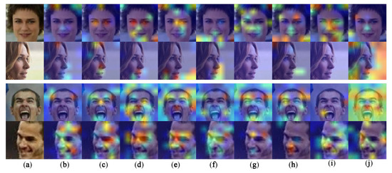
Figure 9.
Two random face image pairs from the CPLFW dataset. The original image pairs are shown in (a), and the corresponding Grad-CAM visualisations for ConvFaceNeXt family members are illustrated from (b) to (e), while for the other previous works are shown from (f) to (j), with all arranged column-wise left to right. (a) Original face image pairs. (b) ConvFaceNeXt_PS. (c) ConvFaceNeXt_PE. (d) ConvFaceNeXt_TS. (e) ConvFaceNeXt_TE. (f) MobileFaceNet [11]. (g) ShuffleFaceNet [12]. (h) ShuffleFaceNet [12]. (i) MobileFaceNetV1 [13]. (j) ProxylessFaceNAS [13].
Finally, two pairs of cross-age face images are shown in Figure 10. The upper image represents a face which is younger than the bottom one. It was observed that most of the ConvFaceNeXt family members highlighted the forehead region of the younger face image. MobileFaceNet highlighted the background region in the upper left corner. Other previous models such as ShuffleFaceNet , ShuffleFaceNet and MobileFaceNetV1 responded to certain face regions. On the other hand, almost the entire image was emphasized by ProxylessFaceNAS, which is undesirable. For the old man’s face image, the ConvFaceNeXt family members showed a good response towards the overall face region. ShuffleFaceNet 1.5× also showed similar performance. Only some parts of the face region were highlighted for MobileFaceNet and MobileFAceNetV1. On the other hand, ShuffleFaceNet 1× emphasized the entire image, in contrast to no excitation from ProxylessFaceNAS. The second pair depicts a younger lady’s face on top and the corresponding older face image at the bottom. It was perceived that the ConvFaceNeXt family was able to emphasise more of the face region compared with the other previous methods for the older face image of the lady.
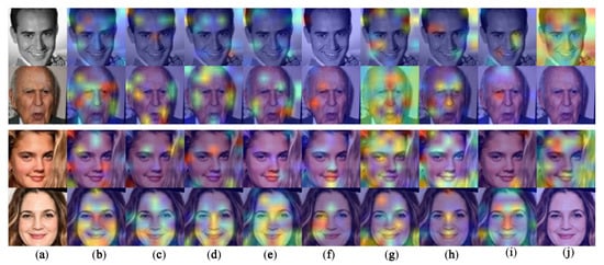
Figure 10.
Two random face image pairs from the CALFW dataset. The original image pairs are shown in (a), and the corresponding Grad-CAM visualisations for ConvFaceNeXt family members are illustrated from (b) to (e), while those for the other previous works are shown from (f) to (j), with all arranged column-wise from left to right. (a) Original face image pairs. (b) ConvFaceNeXt_PS. (c) ConvFaceNeXt_PE. (d) ConvFaceNeXt_TS. (e) ConvFaceNeXt_TE. (f) MobileFaceNet [11]. (g) ShuffleFaceNet [12]. (h) ShuffleFaceNet [12]. (i) MobileFaceNetV1 [13]. (j) ProxylessFaceNAS [13].
From all of the qualitative observations, it was proven that the proposed ConvFaceNeXt models not only highlighted the face region but also emphasized important face parts such as the eyes, nose and mouth. These emphasized face parts are important because these features remain the same regardless of pose and age variations [53]. Moreover, the unnecessary background region was suppressed. This proves that ConvFaceNet family members have better generalisation and discriminative abilities for face recognition tasks.
5. Conclusions
A family of efficient, lightweight face recognition models known as ConvFaceNeXt was introduced. All of the family members are based on the ECN block, with the aim of reducing the FLOP and parameter counts for the whole model. Generally, ConvFaceNeXt consists of three main parts, namely the stem partition, the bottleneck partition and the embedding partition. Ablation studies revealed several important characteristics of ConvFaceNet. First, the linking strategy is used to correlate low-level and high-level features alongside reducing the vanishing gradient problem. Second, the adoption of a depthwise convolution in the ECN block helps with extracting more detailed information in addition to reducing the FLOP and parameter counts. Finally, with less batch normalisations and activation functions, the performance of the models increased. Through quantitative analysis, it was shown that ConvFaceNeXt achieved better verification accuracy in almost all face datasets. From qualitative analysis, ConvFaceNeXt was able to highlight face regions with high excitation on important face parts. Hence, both of these analyses indicate that the ConvFaceNext models showed persistent performance compared with other lightweight face recognition models. In the future, attention mechanisms and other loss functions will be explored to increase the verification accuracy of the ConvFaceNeXt models further. One promising solution is to use a more advanced loss function such as ElasticFace [54]. Instead of a fixed margin, as implemented in ArcFace [32] and CosFace [50], ElasticFace utilizes a random margin. This is to ensure flexible class separability learning that will further boost the generalisability and discriminative capabilities of lightweight face recognition models.
Author Contributions
Conceptualisation, S.C.H., S.A.S. and H.I.; methodology, S.C.H. and H.I.; writing—original draft preparation, S.C.H.; writing—review and editing, S.A.S. and H.I.; supervision, S.A.S. and H.I.; funding acquisition, H.I. All authors have read and agreed to the published version of the manuscript.
Funding
This research was funded by Universiti Sains Malaysia under Research University Grant 1001/PELECT/8014052.
Institutional Review Board Statement
Not applicable.
Informed Consent Statement
Not applicable.
Data Availability Statement
All the presented datasets in this paper can be found through the referenced papers.
Acknowledgments
The authors would like to thank everyone’s support during the implementation of this project, including Guowei Wang for valuable bits of advice, feedback, and sharing of Keras_insightface on https://github.com/leondgarse/Keras_insightface, accessed on 5 March 2022. In addition, S.C.H. would like to express gratitude to the Public Service Department of Malaysia, which offered the Hadiah Latihan Persekutuan (HLP) scholarship for this study.
Conflicts of Interest
The authors declare no conflict of interest.
References
- Taskiran, M.; Kahraman, N.; Erdem, C.E. Face Recognition: Past, Present and Future (A Review). Digit. Signal Process. 2020, 106, 102809. [Google Scholar] [CrossRef]
- Ranjan, R.; Sankaranarayanan, S.; Bansal, A.; Bodla, N.; Chen, J.C.; Patel, V.M.; Castillo, C.D.; Chellappa, R. Deep Learning for Understanding Faces: Machines May Be Just as Good, or Better, than Humans. IEEE Signal Process. Mag. 2018, 35, 66–83. [Google Scholar] [CrossRef]
- Wang, Z.; Chen, J.; Hu, J.; Wang, Z.; Chen, J.; Hu, J. Multi-View Cosine Similarity Learning with Application to Face Verification. Mathematics 2022, 10, 1800. [Google Scholar] [CrossRef]
- Hoo, S.C.; Ibrahim, H. Biometric-based Attendance Tracking System for Education Sectors: A Literature Survey on Hardware Requireemnts. J. Sens. 2019, 2019, 7410478. [Google Scholar] [CrossRef]
- Schroff, F.; Kalenichenko, D.; Philbin, J. Facenet: A Unified Embedding for Face Recognition and Clustering. In Proceedings of the IEEE Conference on Computer Vision and Pattern Recognition, Boston, MA, USA, 7–12 June 2015; pp. 815–823. [Google Scholar]
- Taigman, Y.; Yang, M.; Ranzato, M.A.; Wolf, L. Deepface: Closing the Gap to Human-Level Performance in Face Verification. In Proceedings of the IEEE Conference on Computer Vision and Pattern Recognition, Columbus, OH, USA, 24–27 June 2014; pp. 1701–1708. [Google Scholar]
- Cao, Q.; Shen, L.; Xie, W.; Parkhi, O.M.; Zisserman, A. VGGFace2: A Dataset for Recognising Faces across Pose and Age. In Proceedings of the 2018 13th IEEE International Conference on Automatic Face & Gesture Recognition (FG 2018), Xi’an, China, 15–19 May 2018; pp. 67–74. [Google Scholar]
- Howard, A.G.; Zhu, M.; Chen, B.; Kalenichenko, D.; Wang, W.; Weyand, T.; Andreetto, M.; Adam, H. Mobilenets: Efficient Convolutional Neural Networks for Mobile Vision Applications. arXiv 2017, arXiv:1704.04861. [Google Scholar]
- Sandler, M.; Howard, A.; Zhu, M.; Zhmoginov, A.; Chen, L. MobileNetV2: Inverted Residuals and Linear Bottlenecks. In Proceedings of the IEEE Conference on Computer Vision and Pattern Recognition, Salt Lake City, UT, USA, 18–23 June 2018; pp. 4510–4520. [Google Scholar] [CrossRef]
- Ma, N.; Zhang, X.; Zheng, H.T.; Sun, J. ShuffleNet V2: Practical Guidelines for Efficient CNN Architecture Design. In Computer Vision—ECCV 2018; Ferrari, V., Hebert, M., Sminchisescu, C., Weiss, Y., Eds.; Springer International Publishing: Cham, Switzerland, 2018; pp. 122–138. [Google Scholar]
- Chen, S.; Liu, Y.; Gao, X.; Han, Z. MobileFaceNets: Efficient CNNs for Accurate Real-Time Face Verification on Mobile Devices. In Biometric Recognition. CCBR 2018; Springer: Cham, Switzerland, 2018; pp. 428–438. [Google Scholar]
- Martindez-Díaz, Y.; Luevano, L.S.; Mendez-Vazquez, H.; Nicolas-Diaz, M.; Chang, L.; Gonzalez-Mendoza, M. ShuffleFaceNet: A Lightweight Face Architecture for Efficient and Highly-Accurate Face Recognition. In Proceedings of the 2019 IEEE/CVF International Conference on Computer VisionWorkshop (ICCVW), Seoul, Korea, 27–28 October 2019; pp. 2721–2728. [Google Scholar]
- Martínez-Díaz, Y.; Nicolás-Díaz, M.; Méndez-Vázquez, H.; Luevano, L.S.; Chang, L.; Gonzalez-Mendoza, M.; Sucar, L.E. Benchmarking Lightweight Face Architectures on Specific Face Recognition Scenarios. Artif. Intell. Rev. 2021, 54, 6201–6244. [Google Scholar] [CrossRef]
- Cai, H.; Zhu, L.; Han, S. ProxylessNAS: Direct Neural Architecture Search on Target Task and Hardware. In Proceedings of the 2019 7th International Conference on Learning Representation (ICLR), New Orleans, LA, USA, 6–9 May 2019. [Google Scholar]
- Liu, W.; Zhou, L.; Chen, J. Face Recognition Based on Lightweight Convolutional Neural Networks. Information 2021, 12, 191. [Google Scholar] [CrossRef]
- Boutros, F.; Damer, N.; Fang, M.; Kirchbuchner, F.; Kuijper, A. MixFaceNets: Extremely Efficient Face Recognition Networks. In Proceedings of the 2021 International IEEE Joint Conference on Biometrics (IJCB), Shenzhen, China, 4–7 August 2021. [Google Scholar]
- Tan, M.; Le, Q.V. MixConv: Mixed Depthwise Convolutional Kernels. In Proceedings of the 2019 30th British Machine Vision Conference (BMVC), Cardiff, UK, 9–12 September 2019. [Google Scholar]
- Zhang, P.; Zhao, F.; Liu, P.; Li, M. Efficient Lightweight Attention Network for Face Recognition. IEEE Access 2022, 10, 31740–31750. [Google Scholar] [CrossRef]
- Boutros, F.; Siebke, P.; Klemt, M.; Damer, N.; Kirchbuchner, F.; Kuijper, A. PocketNet: Extreme Lightweight Face Recognition Network Using Neural Architecture Search and Multistep Knowledge Distillation. IEEE Access 2022, 10, 46823–46833. [Google Scholar] [CrossRef]
- Liu, H.; Simonyan, K.; Yang, Y. DARTS: Differentiable Architecture Search. In Proceedings of the 2019 7th International Conference on Learning Representation (ICLR), New Orleans, LA, USA, 6–9 May 2019. [Google Scholar]
- Liu, Z.; Mao, H.; Wu, C.Y.; Feichtenhofer, C.; Darrell, T.; Xie, S. A ConvNet for the 2020s. arXiv 2022, arXiv:2201.03545. [Google Scholar]
- Mondal, M.; Das, B.; Roy, S.D.; Singh, P.; Lall, B.; Joshi, S.D. Adaptive CNN Filter Pruning Using Global Importance Metric. Comput. Vis. Image Underst. 2022, 222, 103511. [Google Scholar] [CrossRef]
- Hupont, I.; Tolan, S.; Gunes, H.; Gómez, E. The Landscape of Facial Processing Applications in The Context of The European AI Act and The Development of Trustworthy Systems. Sci. Rep. 2022, 12, 10688. [Google Scholar] [CrossRef] [PubMed]
- Boutros, F. Efficient and High Performing Biometrics: Towards Enabling Recognition in Embedded Domains. Ph.D. Thesis, Technical University of Darmstadt, Darmstadt, Germany, June 2022. [Google Scholar]
- Minaee, S.; Liang, X.; Yan, S. Modern Augmented Reality: Applications, Trends, and Future Directions. arXiv 2022, arXiv:2202.09450. [Google Scholar]
- Shah, S.W.; Kanhere, S.S. Recent Trends in User Authentication—A Survey. IEEE Access 2019, 7, 112505–112519. [Google Scholar] [CrossRef]
- Brown, D. Mobile Attendance based on Face Detection and Recognition using OpenVINO. In Proceedings of the 2021 International Conference on Artificial Intelligence and Smart Systems (ICAIS), Coimbatore, India, 25–27 March 2021. [Google Scholar]
- Shaukat, Z.; Akhtar, F.; Fang, J.; Ali, S.; Azeem, M. Cloud based Face Recognition for Google Glass. In Proceedings of the 2018 International Conference on Computing and Artificial Intelligence (ICCAI), Chengdu, China, 12–14 March 2018. [Google Scholar]
- Deng, J.; Guo, J.; Zhang, D.; Deng, Y.; Lu, X.; Shi, S. Lightweight Face Recognition Challenge. In Proceedings of the IEEE International Conference on Computer Vision (ICCV), Seoul, Korea, 27 October–2 November 2019. [Google Scholar]
- Deng, J.; Dong, W.; Socher, R.; Li, L.J.; Li, K.; Li, F.F. ImageNet: A Large-Scale Hierarchical Image Database. In Proceedings of the 2009 IEEE Conference on Computer Vision and Pattern Recognition, Miami, FL, USA, 20–25 June 2009; pp. 248–255. [Google Scholar] [CrossRef]
- Hu, J.; Shen, L.; Albanie, S.; Sun, G.; Wu, E. Squeeze-and-Excitation Networks. IEEE Trans. Pattern Anal. Mach. Intell. 2020, 42, 2011–2023. [Google Scholar] [CrossRef] [PubMed]
- Deng, J.; Guo, J.; Yang, J.; Xue, N.; Cotsia, I.; Zafeiriou, S.P. ArcFace: Additive Angular Margin Loss for Deep Face Recognition. IEEE Trans. Pattern Anal. Mach. Intell. 2021, 44, 5962–5979. [Google Scholar] [CrossRef]
- Xiao, J.; Jiang, G.; Liu, H. A Lightweight Face Recognition Model based on MobileFaceNet for Limited Computation Environment. EAI Endorsed Trans. Internet Things 2022, 7. [Google Scholar] [CrossRef]
- Wang, Q.; Wu, B.; Zhu, P.; Li, P.; Zuo, W.; Hu, Q. ECA-Net: Efficient Channel Attention for Deep Convolu-tional Neural Networks. In Proceedings of the 2020 IEEE/CVF Conference on Computer Vision and Pattern Recognition (CVPR), Seattle, WA, USA, 13–19 June 2020. [Google Scholar] [CrossRef]
- Jia, W.; Ren, Q.; Zhao, Y.; Li, S.; Min, H.; Chen, Y. EEPNet: An Efficient and Effective Convolutional Neural Network for Palmprint Recognition. Pattern Recognit Lett. 2022, 159, 140–149. [Google Scholar] [CrossRef]
- Bansal, A.; Nanduri, A.; Castillo, C.D.; Ranjan, R.; Chellappa, R. UMDFaces: An Annotated Face Dataset for Training Deep Networks. In Proceedings of the IEEE International Joint Conference on Biometrics (IJCB), Denver, CO, USA, 1–4 October 2017; pp. 464–473. [Google Scholar] [CrossRef]
- Yi, D.; Lei, Z.; Liao, S.; Li, S. Learning Face Representation from Scratch. arXiv 2014, arXiv:1411.7923. [Google Scholar]
- Parkhi, O.M.; Vedaldi, A.; Zisserman, A. Deep Face Recognition. In Proceedings of the BMVC 2015—British Machine Vision Conference, Swansea, UK, 7–10 September 2015. [Google Scholar]
- Zhang, K.; Zhang, Z.; Li, Z.; Qiao, Y. Joint Face Detection and Alignment Using Multitask Cascaded Convolutional Networks. IEEE Signal Process. Lett. 2016, 23, 1499–1503. [Google Scholar] [CrossRef]
- Wang, Q.; Zhang, P.; Xiong, H.; Zhao, J. Face.EvoLVe: A Cross-Platform Library for High-Performance Face Analytics. Neurocomputing 2022, 494, 443–445. [Google Scholar] [CrossRef]
- Huang, G.B.; Mattar, M.; Berg, T.; Learned-Miller, E. Labeled Faces in the Wild: A Database for Studying Face Recognition in Unconstrained Environments. In Proceedings of the Workshop on Faces in ‘Real-Life’ Images: Detection, Alignment, and Recognition, Marseille, France, 12–18 October 2008. [Google Scholar]
- Zheng, T.; Deng, W.; Hu, J. Cross-Age LFW: A Database for Studying Cross-Age Face Recognition in Unconstrained Environments. arXiv 2017, arXiv:1708.08197. [Google Scholar] [CrossRef]
- Zheng, T.; Deng, W. Cross-Pose LFW: A Database for Studying Cross-Pose Face Recognition in Unconstrained Environments; Technical Report; Beijing University of Posts and Telecommunications: Beijing, China, 2018; Available online: http://www.whdeng.cn/CPLFW/Cross-Pose-LFW.pdf (accessed on 5 January 2022).
- Sengupta, S.; Chen, J.C.; Castillo, C.; Patel, V.M.; Chellappa, R.; Jacobs, D.W. Frontal to Profile Face Verification in the Wild. In Proceedings of the 2016 IEEE Winter Conference on Applications of Computer Vision (WACV), Lake Placid, NY, USA, 7–9 March 2016; pp. 1–9. [Google Scholar] [CrossRef]
- Moschoglou, S.; Papaioannou, A.; Sagonas, C.; Deng, J.; Kotsia, I.; Zafeiriou, S. AgeDB: The First Manually Collected, In-the-Wild Age Database. In Proceedings of the IEEE Conference on Computer Vision and Pattern Recognition Workshops (CVPRW), Honolulu, HI, USA, 21–26 June 2017; pp. 51–59. [Google Scholar] [CrossRef]
- Whitelam, C.; Taborsky, E.; Blanton, A.; Maze, B.; Adams, J.; Miller, T.; Kalka, N.; Jain, A.K.; Duncan, J.A.; Allen, K.; et al. IARPA Janus Benchmark-B Face Dataset. In Proceedings of the IEEE Conference on Computer Vision and Pattern Recognition Workshops (CVPRW), Honolulu, HI, USA, 21–26 June 2017; pp. 592–600. [Google Scholar] [CrossRef]
- Maze, B.; Adams, J.; Duncan, J.A.; Kalka, N.; Miller, T.; Otto, C.; Jain, A.K.; Niggel, W.T.; Anderson, J.; Cheney, J.; et al. IARPA Janus Benchmark-C: Face Dataset and Protocol. In Proceedings of the 2018 International Conference on Biometrics (ICB), Queensland, Australia, 20–23 February 2018; pp. 158–165. [Google Scholar] [CrossRef]
- Russell, S.; Norvig, P. Artifcial Intelligence: A Modern Approach, 4th Global ed.; Pearson Education Limited: London, UK, 2022. [Google Scholar]
- Wang, Z.; Bai, Y.; Zhou, Y.; Xie, C. Can CNNs Be More Robust Than Transformers? arXiv 2022, arXiv:2206.03452. [Google Scholar] [CrossRef]
- Wang, H.; Wang, Y.; Zhou, Z.; Ji, X.; Gong, D.; Zhou, J.; Li, Z.; Liu, W. CosFace: Large Margin Cosine Loss for Deep Face Recognition. In Proceedings of the IEEE Conference on Computer Vision and Pattern Recognition (CVPR), Salt Lake City, UT, USA, 18–22 June 2018; pp. 5265–5274. [Google Scholar]
- Selvaraju, R.R.; Cogswell, M.; Das, A.; Vedantam, R.; Parikh, D.; Batra, D. Grad-CAM: Visual Explanations from Deep Networks via Gradient-Based Localization. Int. J. Comput. Vis. 2020, 128, 336–359. [Google Scholar] [CrossRef]
- Zhao, J.; Han, J.; Shao, L. Unconstrained Face Recognition Using a Set-to-Set Distance Measure on Deep Learned Features. IEEE Trans. Circuits Syst. Video Technol. 2018, 28, 2679–2689. [Google Scholar] [CrossRef]
- Wang, Q.; Guo, G. LS-CNN: Characterizing Local Patches at Multiple Scales for Face Recognition. IEEE Trans. Inf. Forensics Secur. 2019, 15, 1640–1653. [Google Scholar] [CrossRef]
- Boutros, F.; Damer, N.; Kirchbuchner, F.; Kuijper, A. ElasticFace: Elastic Margin Loss for Deep Face Recogni-tion. In Proceedings of the IEEE Conference on Computer Vision and Pattern Recognition Workshops (CVPRW), New Orleans, LA, USA, 19–20 June 2022; pp. 1577–1586. [Google Scholar] [CrossRef]
Publisher’s Note: MDPI stays neutral with regard to jurisdictional claims in published maps and institutional affiliations. |
© 2022 by the authors. Licensee MDPI, Basel, Switzerland. This article is an open access article distributed under the terms and conditions of the Creative Commons Attribution (CC BY) license (https://creativecommons.org/licenses/by/4.0/).