Collision Avoidance Problem of Ellipsoid Motion

Abstract

This paper studies the problem of target control and how a virtual ellipsoid can avoid the static obstacle. During the motion to the target set, the virtual ellipsoid can achieve a motion under collision avoidance by keeping the distance between the ellipsoid and obstacle. We present solutions to this problem in the class of closed-loop (feedback) controls based on Hamilton–Jacobi–Bellman (HJB) equation. Simulation results verify the validity and effectiveness of our algorithm.

1. Introduction

Control problems play an important role in modern scientific research. Data-driven control and fuzzy control problems for both linear and nonlinear system remain a popular task, and many theoretical researches have been carried out, such as Virtual Reference Feedback Tuning (VRFT) [1] and indirect adaptive iterative learning control (iAILC) scheme [2]. Formation control is one of the significant interest topics in the research of multi-agent system (MAS). Formation control can be realized by using various types of vehicles, such as unmanned aerial vehicles, mobile robots, underwater vehicles and so on. It has found a wide range of applications including military, aerospace, industry, etc.

The research of formation control mainly includes the following aspects: formation generation, formation maintenance, formation switching, formation avoidance and formation adaptive problems. The approaches to formation control are roughly categorized as leader-follower [3,4,5,6], behavioral [7,8], virtual structure [9,10] and artificial potential field [11,12].

Generally speaking, the collision avoidance problem in formation control includes two aspects. On the one hand, the members of MAS should avoid collision with each other in the process of motion. On the other hand, MAS should avoid collision with obstacles. A lot of research has been done in the field of obstacle avoidance algorithm. Many of them are based on artificial potential field [13,14]. Sometimes the control is realized with genetic algorithms (GA) [15], which is a powerful tool based on models of natural selection and evolution and allow an exhaustive search over large spaces. In [16] a visibility graph approach is used, while in [17] collision avoidance is achieved using A-Star algorithm.

In [18], Kurzhanski presents a theoretical framework of formation control approach for MAS based on the virtual ellipsoidal motions. This motion is achieved by means of a virtual ellipsoidal container inside which the members are assumed to be a sphere with safety volume. Kurzhanski considers the motions of MAS within the container so that the motions reach the target set together with the virtual container containing them. Therefore, his work considers about moving to the target set while avoiding collisions. In light of the above discussion, the motions of virtual ellipsoids can be fully portrayed by the linear differential equation satisfied with the coordinates of the center and the configuration matrix. Kurzhanski proposes the motion trajectory of virtual ellipsoid and MAS based on a suitable value function and dynamic programming method, thereby giving a solution scheme for MAS. Kurzhanski’s related work can be found in the literature [19,20,21,22,23,24,25,26].

In fact, we can regard Kurzhanski’s approach to formation control of MAS based on virtual ellipsoid as an improvement of virtual structure method. Traditional virtual structure views the formation of MAS as virtual rigid structure, in which each intelligent tracks a fixed virtual point motion on a rigid structure. This rigid structure limits on the application range of the method. While the formation control approach based on virtual ellipsoid motion not only inherits the advantage that it is easy to describe system behavior as a whole and can obtain higher-cell control accuracy from traditional virtual structures, but also fully compensates for the defects of rigid motion in traditional virtual structures.

Based on the work of Kurzhanski, this paper achieves the optimal target control problem based on virtual ellipsoid. This means that we should obtain optimal controls for the ellipsoid center and configuration matrix, which is significantly different from the traditional virtual structure method. Then, taking the actual situation of obstacle avoidance for formation control into account, we present the integration of virtual ellipsoid volume constraint, ellipsoid center constraint and configuration constraint into value function. Thereby we achieve optimal control to ellipsoid. Finally, we verify the effectiveness of our method by numerical simulations.

2. Statement of the Problem

We start this section with the definition of an ellipsoid in ${ℝ}^n$.

Definition 1

([22]). A nondegenerate ellipsoid $\epsilon (q,Q)$ in ${ℝ}^n$ with center $q\in {ℝ}^n$ and configuration matrix $Q\in {ℝ}^{n\times n}$ is the set

$$\epsilon (q,Q)=\{p\in {ℝ}^n:\langle p-q,Q^{-1}(p-q)\rangle \le 1\},$$

where $Q$ is positive definite. Here $\langle \cdot ,\cdot \rangle$ denotes inner product of two vector and $Q^{-1}$ is the inverse matrix of $Q$.

On the time interval $[t_0,\theta ]$, consider the virtual ellipsoidal motions of type

$$E_c[t]=\epsilon (q(t),Q(t)),$$

with $q\left(t\right)\in {ℝ}^n$ and positive definite matrix function $Q(t)\in {ℝ}^{n\times n}$ which are continuous at time $t$. $E_c[t](t\in [t_0,\theta ])$ is referred as an ellipsoidal tube.

Now consider an ellipsoidal tube $E_c[t](t\in [t_0,\theta ])$ with the following systems [23]:

$$\dot{q}(t)=A_q(t)q(t)+B_q(t)u(t,q),\hspace{1em}q(t_0)=q_0,$$

(1)

$$\dot{Q}(t)=T(t)Q(t)+Q(t)T^{\prime }(t)+B_Q(t)U(t,Q){B^{\prime }}_Q(t),\hspace{1em}Q(t_0)=Q_0,$$

(2)

where $u(t,q)\in {ℝ}^{m_1}$ controls the trajectory of $q(t)$ and $U(t,Q)\in {ℝ}^{m_2\times m_2}$ controls the configuration matrix $Q(t)$. The matrix parameters $A_q(t)\in {ℝ}^{n\times n}$, $B_q(t)\in {ℝ}^{n\times m_1}$, $B_Q(t)\in {ℝ}^{n\times m_2}$, $T(t)\in {ℝ}^{n\times n}$ are assumed to be continuously differentiable at time $t$, and $T(t)$ is symmetric matrix. Here the prime of a matrix stands for the transposition of the matrix. The solvable conditions of system (1) and (2) have been discussed in [22] and Appendix B.

Next the used control constraint, geometric constraints, barrier constraint for the systems (1) and (2) are stated and the main problem is explained.

2.1. Control Constraint

Assume the admissible control sets to be $\mathit{u}(t,q)\subseteq {ℝ}^{m_1}$ and $\mathit{U}(t,Q)\subseteq {ℝ}^{m_2\times m_2}$, where $\mathit{u}(t,q)$ and $\mathit{U}(t,Q)$ are given compact convex sets. For any control $u(t,q)\in \mathit{u}(t,q)$ and $U(t,Q)\in \mathit{U}(t,Q)$, we have

$${\displaystyle \underset{t_0}{\overset{\theta }{\int }}(\langle u(t,q),u(t,q)\rangle )+[U(t,Q),U(t,Q)]dt\le {\mu }^2,}$$

(3)

where the constant $\mu >0$. Here $[U,U]=\mathrm{tr}(U^{\prime }U)$ denotes the inner product of two matrices.

2.2. State Constraints

Systems (1) and (2) are also considered under the additional state constraints

$$[Q(t),Q(t)]\le {\delta }^2,$$

(4)

$${\sigma }^2\le [Q(t),Q(t)],$$

(5)

where constants $\delta >\sigma >0$. Note that inequality (4) defines a convex constraint, and inequality (5) defines a constraint complementary to a convex one. These inequalities restrict the possible size of an ellipsoid with configuration matrix $Q(t)$. Condition $(4)$ implies that $E_c[t]$ is contained in a ball with a radius of $\delta /n$ and condition $(5)$ implies that $E_c[t]$ contains a ball with a radius of $\sigma /n$.

2.3. Barrier Constraint

In this paper, obstacles are also regarded as virtual ellipsoids. Let the static ellipsoid $B^{\ast }=\epsilon (q^{\ast },Q^{\ast })$ be fixed obstacle on the path of the ellipsoid motion, where $q^{\ast }\in {ℝ}^n$ is the center and $Q^{\ast }\in {ℝ}^{n\times n}$ is the configuration matrix which is positive definite. Let the eigenvalues of $Q^{\ast }$ be ${\lambda }_1,{\lambda }_2,\dots ,{\lambda }_n$, where ${\lambda }_i>0, i=1,2,\dots ,n$. Denote

$$\max \{{\lambda }_i|i=1,\dots ,n\}={\left(\frac{d}{2}\right)}^2,$$

where $d/2$ is the radius of the smallest n-dimensional ball that includes $B^{\ast }$. While moving, $E_c[t]$ has to avoid obstacle $B^{\ast }$. We realize a motion under collision avoidance by keeping the distance between the $E_c[t]$ and obstacle $B^{\ast }$. Actually, we only limit the distance between $q(t)$ and $q^{\ast }$ to be greater than $\delta /\sqrt{n}+d/2$. Letting $r=\delta /\sqrt{n}+d/2$, we have

$$\langle q(t)-q^{\ast },q(t)-q^{\ast }\rangle \ge r^2.$$

(6)

2.4. Main Problem

With the ellipsoid $E_M=\epsilon (m,M)$ being the target state, where $m\in {ℝ}^n$ is center, $M\in {ℝ}^{n\times n}$ is configuration matrix and positive definite. Let the target set

$$M_{\omega }=\{(q,Q)\in {ℝ}^n\times {ℝ}^{n\times n}|\langle q-m,q-m\rangle +[Q-M,Q-M]\le {\omega }^2,\omega >0\}$$

(7)

be given in the form of a neighborhood of the ellipsoid $E_M$.

This paper deals with the control problem of ellipsoid motion. The control objective in this paper is to drive the system to arrive at the target set, with the collision avoidance. By summarizing the above descriptions, we formulate the solution for systems $(1)$ and $(2)$ as follows.

Problem 1.

Given equation systems $(1)$ and $(2)$ on an interval $[t_0,\theta ]$, let an initial state be $\{t_0,q(t_0),Q(t_0)\}$, therefore we get the initial ellipsoid $E_c[t_0]=\epsilon (q(t_0),Q(t_0))$. Find feedback controls $u\left(t,q\right)$ and $U(t,Q)$ that transfer the ellipsoid $E_c[t]$ from the state $E_c[t_0]$ into terminal set $M_{\omega }$ under the constraints (3)–(6).

In order to find the optimal feedback controls $u\left(t,q\right)$ and $U(t,Q)$ of problem, we define the objective function

$$\begin{array}{ll}\mathrm{\Psi }(u(\cdot ),U(\cdot ))& ={\displaystyle \underset{t_0}{\overset{\theta }{\int }}({\alpha }_1(\langle u(t,q),u(t,q\rangle +[U(t,Q),U(t,Q)])+{\alpha }_2({\delta }^2-[Q(t),Q(t)])}\\ & +{\alpha }_3([Q(t),Q(t)]-{\sigma }^2)-\beta \langle q(t)-q^{\ast },q(t)-q^{\ast }\rangle )dt\\ & +\gamma (\langle q(\theta )-m,q(\theta )-m\rangle +[Q(\theta )-M,Q(\theta )-M]),\end{array}$$

(8)

where constants ${\alpha }_1,{\alpha }_2,{\alpha }_3,\beta ,\gamma$ are referred to as weight coefficients.

In this paper, we use the distance between the ellipsoid and the obstacle to constrain the objective function, in which the movement of the ellipsoid is restricted by term $\langle q(t)-q^{\ast },q(t)-q^{\ast }\rangle$ to realize collision avoidance.

3. Solutions Developed

In this section, we use dynamic programming method to solve the above-mentioned optimal control problem. The value function defined on the trajectories of systems (1) and (2) is

$$V_E(t,q,Q)=\underset{u,U}{\min }\{\mathrm{\Psi }(u(\cdot ),U(\cdot ))|q(t)=q,Q(t)=Q\}.$$

For fixed ${\alpha }_1,{\alpha }_2,{\alpha }_3,\beta ,\gamma$, we obtain ([24])

$$W[t]=\left\{q(t),Q(t)|V_E(t,q,Q)\le 1\right\},$$

where $W[t]$ is the backward reach set relative to $M_{\omega }$ under the constraints (3)–(6), i.e., the set of points $\{q(t),Q(t)\}$ for which there exist controls $u(t,q)$ and $U(t,Q)$ that steers $E_c[t]$ to $E_{\omega }$ under the constraints (3)–(6). The value function for this problem is

$$V_E(t,q,Q)=\underset{{\alpha }_1,{\alpha }_2,{\alpha }_3,\gamma }{\max }\underset{\beta }{\min }\{V_E(t,q,Q)|{\alpha }_1,{\alpha }_2,{\alpha }_3,\beta ,\gamma \}$$

over all $\{{\alpha }_1,{\alpha }_2,{\alpha }_3,\beta ,\gamma \ge 0: {\alpha }_1{\mu }^{-2}+{\alpha }_2{\delta }^{-2}+{\alpha }_3{\sigma }^{-2}+\beta r^{-2}+\gamma {\omega }^{-2}=1\}$. The meanings of the parameters have been listed in the

Table 1. Details of all the parameters.

${\alpha }_1$	Constraining controls of the ellipsoid
${\alpha }_2$	Constraining the volume of the ellipsoid by constraining an upper bound on the norm of the ellipsoid configuration matrix
${\alpha }_3$	Constraining the volume of the ellipsoid by constraining a lower bound on the norm of the ellipsoid configuration matrix
$\beta$	Constraining the distance between the center of ellipsoid and the obstacle
$\gamma$	Constraining the distance between the ellipsoid and the target

below.

We can substitute the weight coefficients of this problem into value function to obtain the corresponding control. The obtained solutions will depend on $\mu ,\delta ,\sigma ,r,\omega$.

Solving this problem is equivalent to minimizing this value function

$$\begin{array}{ll}{V}_E(t,q,Q)& =\underset{u,U}{\min }{\displaystyle \underset{t}{\overset{\theta }{\int }}({\alpha }_1(\langle u(\tau ,q),u(\tau ,q)\rangle +[U(\tau ,Q),U(\tau ,Q)])+{\alpha }_2({\delta }^2-[Q(\tau ),Q(\tau )])}\\ & +{\alpha }_3([Q(\tau ),Q(\tau )]-{\sigma }^2)-\beta \langle q(\tau )-q^{\ast },q(\tau )-q^{\ast }\rangle )d\tau \\ & +\gamma (\langle q(\theta )-m,q(\theta )-m\rangle +[Q(\theta )-M,Q(\theta )-M]).\end{array}$$

For the convenience of calculation, we rewrite the system $(2)$ in vector form [25]. Let $A=(a_{ij})\in {ℝ}^{n\times n}$, introducing the notation

$$\overline{A}={[a_{11},a_{12},\dots ,a_{1n},a_{21},a_{22},\dots ,a_{2n},\dots ,a_{n1},a_{n2},\dots ,a_{nn}]}^{\prime }.$$

Let $B=(b_{ij})\in {ℝ}^{n\times n}$, the Kronecker product of matrices is denoted as

$$A\otimes B=\left[\begin{array}{ccc}{a}_{11}B& \cdots & a_{1n}B\\ ⋮& \ddots & ⋮\\ a_{n1}B& \cdots & a_{nn}B\end{array}\right]\in {ℝ}^{n^2\times n^2}.$$

Using the identity $\overline{AXB}=(A\otimes B^{\prime })\overline{X}$, then system $(2)$ can be rewritten as

$$\dot{\overline{Q}}=(T(t)\otimes I)\overline{Q}+(I\otimes T(t))\overline{Q}+(B_Q(t)\otimes B_Q(t))\overline{U}(t,Q).$$

Denoting $\mathit{A}(t)=T(t)\otimes I+I\otimes T(t)$, $\mathit{B}(t)=B_Q(t)\otimes B_Q(t)$, we obtain the relation

$$\dot{\overline{Q}}=\mathit{A}(t)\overline{Q}+\mathit{B}(t)\overline{U}(t,Q).$$

Then the value function can be replaced by the form

$$\begin{array}{ll}{V}_E(t,q,Q)& =\underset{u,\overline{U}}{\min }{\displaystyle \underset{t}{\overset{\theta }{\int }}({\alpha }_1(\langle u(\tau ,q),u(\tau ,q)\rangle +\langle \overline{U}(\tau ,Q),\overline{U}(\tau ,Q)\rangle )+{\alpha }_2({\delta }^2-\langle \overline{Q}(\tau ),\overline{Q}(\tau )\rangle )}\\ & +{\alpha }_3(\langle \overline{Q}(\tau ),\overline{Q}(\tau )\rangle -{\sigma }^2)-\beta \langle q(\tau )-q^{\ast },q(\tau )-q^{\ast }\rangle )d\tau \\ & +\gamma (\langle q(\theta )-m,q(\theta )-m\rangle +\langle \overline{Q}(\theta )-\overline{M},\overline{Q}(\theta )-\overline{M}\rangle ).\end{array}$$

(9)

Then function $(9)$ derives a solution to the HJB equation ([27])

$$\begin{array}{ll}\frac{\partial V_E}{\partial t}& +\underset{u,U}{\min }\{\langle \frac{\partial V_E}{\partial q},A_q(t)q+B_q(t)u(t,q)\rangle +\langle \frac{\partial V_E}{\partial \overline{Q}},\mathit{A}(t)\overline{Q}+\mathit{B}(t)\overline{U}(t,Q)\rangle \\ & +{\alpha }_1(\langle u(t,q),u(t,q)\rangle +\overline{U}(t,Q),\overline{U}(t,Q))+{\alpha }_2({\delta }^2-\langle \overline{Q},\overline{Q}\rangle )\\ & +{\alpha }_3(\langle \overline{Q},\overline{Q}\rangle -{\sigma }^2)-\beta \langle q-q^{\ast },q-q^{\ast }\rangle \}=0,\end{array}$$

(10)

with the boundary condition

$$V_E(\theta ,q(\theta ),Q(\theta ))=\gamma (\langle q(\theta )-m,q(\theta )-m\rangle +\langle \overline{Q}(\theta )-\overline{M},\overline{Q}(\theta )-\overline{M}\rangle ).$$

(11)

The solution to Equation $(10)$ is given as Equation $(9)$. Denoting

$$\begin{array}{ll}H(t,u(t),\overline{U}(t))& =\langle \frac{\partial V_E}{\partial q},A_q(t)q+B_q(t)u(t,q)\rangle +\langle \frac{\partial V_E}{\partial \overline{Q}},\mathit{A}(t)\overline{Q}+\mathit{B}(t)\overline{U}(t,Q)\rangle \\ & +{\alpha }_1(\langle u(t,q),u(t,q)\rangle +\overline{U}(t,Q),\overline{U}(t,Q))+{\alpha }_2({\delta }^2-\langle \overline{Q},\overline{Q}\rangle )\\ & +{\alpha }_3(\langle \overline{Q},\overline{Q}\rangle -{\sigma }^2)-\beta \langle q-q^{\ast },q-q^{\ast }\rangle \}=0.\end{array}$$

Then Equation $(10)$ is equivalent to

$$\left\{\begin{array}{l}\frac{\partial V_E}{\partial t}+H(t,u,\overline{U})=0,\\ \frac{\partial H(t,u,\overline{U})}{\partial u}=0,\\ \frac{\partial H(t,u,\overline{U})}{\partial \overline{U}}=0.\end{array}\right.$$

First, we have the partial derivative of $H(t,u,\overline{U})$ with respect to $u$ and $U$

$$u(t,q)=-\frac{1}{2{\alpha }_1}{B^{\prime }}_q(t)\frac{\partial V_E}{\partial q},$$

(12)

$$\overline{U}(t,Q)=-\frac{1}{2{\alpha }_1}{\mathit{B}}^{\prime }(t)\frac{\partial V_E}{\partial \overline{Q}}.$$

(13)

Substituting $(12)$, $(13)$ into $\frac{\partial V_E}{\partial t}+H(t,u,\overline{U})=0$, Equation $(10)$ can be rewritten as

$$\begin{array}{ll}\frac{\partial V_E}{\partial t}& +\langle \frac{\partial V_E}{\partial q},A_q(t)q\rangle -\frac{1}{4{\alpha }_1}\langle \frac{\partial V_E}{\partial q},B_q(t){B_q}^{\prime }(t)\frac{\partial V_E}{\partial q}\rangle +\langle \frac{\partial V_E}{\partial \overline{Q}},\mathit{A}(t)\overline{Q}\rangle \\ & -\frac{1}{4{\alpha }_1}\langle \frac{\partial V_E}{\partial \overline{Q}},\mathit{B}(t){\mathit{B}}^{\prime }(t)\frac{\partial V_E}{\partial \overline{Q}}\rangle +{\alpha }_2({\delta }^2-\langle \overline{Q},\overline{Q}\rangle )+{\alpha }_3(\langle \overline{Q},\overline{Q}\rangle -{\sigma }^2)\\ & -\beta \langle q-q^{\ast },q-q^{\ast }\rangle =0.\end{array}$$

(14)

The resulting expression is a quadratic form in the state coordinates and the spatial derivatives of the value function. The latter permits one to seek the value function in quadratic form as well,

$$V_E(t,q,Q)=\langle q,p(t)q\rangle +[q,k(t)]+[Q,P(t)Q]+[Q,K(t)]+s(t),$$

the above equation is equivalent to (16)

$$V_E(t,q,Q)=\langle q,p(t)q\rangle +\langle q,k(t)\rangle +\langle \overline{Q},\mathit{P}(t)\overline{Q}\rangle +\langle \overline{Q},\mathit{K}(t)\rangle +s(t),$$

(15)

where $\mathit{P}(t)$ and $p(t)$ are symmetric positive definite, $\mathit{P}(t)=P(t)\otimes I_{n\times n}$, $\mathit{K}(t)=\overline{K}(t)$. We have the partial derivative of function $V_E(t,q,Q)$ with respect to $t$, $q$ and $\overline{Q}$

$$\begin{array}{c}\frac{\partial V_E}{\partial t}=\langle q,\dot{p}(t)q\rangle +\langle q,\dot{k}(t)\rangle +\langle \overline{Q},\dot{\mathit{P}}(t)\overline{Q}\rangle +\langle \overline{Q},\dot{\mathit{K}}(t)\rangle +\dot{s}(t),\\ \frac{\partial V_E}{\partial q}=2p(t)q+k(t),\hspace{1em}\hspace{1em}\frac{\partial V_E}{\partial \overline{Q}}=2\mathit{P}(t)\overline{Q}+\mathit{K}(t).\end{array}$$

Equations $(12)$ and $(13)$ can be rewritten as

$$u(t,q)=-\frac{1}{2{\alpha }_1}{B^{\prime }}_q(t)(2p(t)q+k(t)),$$

(16)

$$\overline{U}(t,Q)=-\frac{1}{2{\alpha }_1}{\mathit{B}}^{\prime }(t)(2\mathit{P}(t)\overline{Q}+\mathit{K}(t)).$$

(17)

By substituting Equation $(15)$ into Equations $(11)$ and $(14)$, we thereby obtain equations for the parameters of the form $(15)$, such as

$$\begin{array}{l}\dot{p}(t)+2p(t)A_q(t)-\frac{1}{{\alpha }_1}p(t)B_q(t){B^{\prime }}_q(t)p(t)-\beta I_{n\times n}=0,p(\theta )=\gamma I_{n\times n},\\ \dot{k}(t)+{A^{\prime }}_q(t)k(t)-\frac{1}{{\alpha }_1}p(t)B_q(t){B^{\prime }}_q(t)k(t)+2\beta q^{\ast }=0,k(\theta )=-2\gamma m,\\ \dot{\mathit{P}}(t)+2\mathit{P}(t)\mathit{A}(t)-\frac{1}{{\alpha }_1}\mathit{P}(t)\mathit{B}(t){\mathit{B}}^{\prime }(t)\mathit{P}(t)-({\alpha }_2-{\alpha }_3)I_{n^2\times n^2}=0,\mathit{P}(\theta )=\gamma I_{n^2\times n^2},\\ \dot{\mathit{K}}(t)+{\mathit{A}}^{\prime }(t)\mathit{K}(t)-\frac{1}{{\alpha }_1}\mathit{P}(t)\mathit{B}(t){\mathit{B}}^{\prime }(t)\mathit{K}(t)=0,\mathit{K}(\theta )=-2\gamma \overline{M},\\ \dot{s}(t)-\frac{1}{4{\alpha }_1}\langle k(t),k(t)\rangle -\frac{1}{4{\alpha }_1}\langle \mathit{K}(t),\mathit{K}(t)\rangle +{\alpha }_2{\delta }^2-{\alpha }_3{\sigma }^2-\beta \langle q^{\ast },q^{\ast }\rangle =0,\\ s(\theta )=\gamma (\langle m,m\rangle +\langle \overline{M},\overline{M}\rangle ).\end{array}$$

(18)

Under the condition of continuous differentiability of the matrix parameters of the systems $(1)$ and $(2)$, the functions $(10)$ and $(11)$ have a unique classical solution. We have thereby proved the following assertion.

Theorem 1.

The value function $(15)$ in which the parameters are determined by systems $(18)$ specifies a solution to Problem 1. In this case, the optimal controls $u(t,q)$ and $U\left(t,\overline{Q}\right)$ are given by $(16)$ and $(17)$.

Since the above formulas involve nonlinear terms, it is difficult for us to obtain analytical expressions even for this relatively simple model, so we focus on numerical solutions. In a similar way as [26], forward Explicit Euler method (in reverse time) is introduced to perform numerical discretization, and the ellipsoid trajectory tube is obtained by MATLAB software. The corresponding implemented algorithm has been attached in Appendix A.

4. Numerical Simulation

In order to verify the control method of collision avoidance proposed in this paper, numerical simulation results are presented in this section. The simulation includes two cases: the presence of obstacle constraint and the absence of obstacle constraint.

Consider the following parameters of the dynamics $(1)$ and $(2)$ of the center and the configuration matrix for a solution that uses Equation $(8)$.

$$\begin{array}{c}{q}_0={[0,0]}^{\prime },\hspace{1em}{Q}_0=\left[\begin{array}{cc}0.005& 0\\ 0& 0.005\end{array}\right],\hspace{1em}{t}_0=0,\hspace{1em}\theta =1,\\ A_q=\left[\begin{array}{cc}9t& -\frac{6}{20}\\ -\frac{6}{20}& 9t\end{array}\right],\hspace{1em}{B}_q=\left[\begin{array}{cc}\frac{t}{3}& \frac{t}{3}\\ \frac{t}{3}& \frac{t}{3}\end{array}\right],\hspace{1em}T=\left[\begin{array}{cc}-t& \sqrt{2}\\ \sqrt{2}& -t\end{array}\right],\hspace{1em}{B}_Q=\left[\begin{array}{cc}\cos \left(\pi t\right)& -\sin \left(\pi t\right)\\ \sin \left(\pi t\right)& \cos \left(\pi t\right)\end{array}\right].\end{array}$$

The center and the configuration matrix of the target ellipse are given as

$$m={[1,1]}^{\prime },\hspace{1em}M=\left[\begin{array}{cc}0.005& 0\\ 0& 0.005\end{array}\right].$$

The center and the configuration matrix of the obstacle are described as

$$q^{\ast }={[0.5,0.5]}^{\prime },\hspace{1em}{Q}^{\ast }=\left[\begin{array}{cc}0.005& 0\\ 0& 0.005\end{array}\right].$$

Now we choose the parameters of Equations (3)–(7) as follows

$${\mu }^2={\omega }^2=r^2=0.2, {\delta }^2=0.28, {\sigma }^2=0.1.$$

Omitting the presence of obstacle constraint, we consider Equation $(8)$ with the parameters specified as

$${\alpha }_1=0.019, {\alpha }_2=0.075, {\alpha }_3=0.035, \beta =0, \gamma =0.057.$$

Considering the presence of obstacle constraint, the parameters in Equation $(8)$ are defined as follows

$${\alpha }_1=0.012, {\alpha }_2=0.057, {\alpha }_3=0.029, \beta =0.048, \gamma =0.04.$$

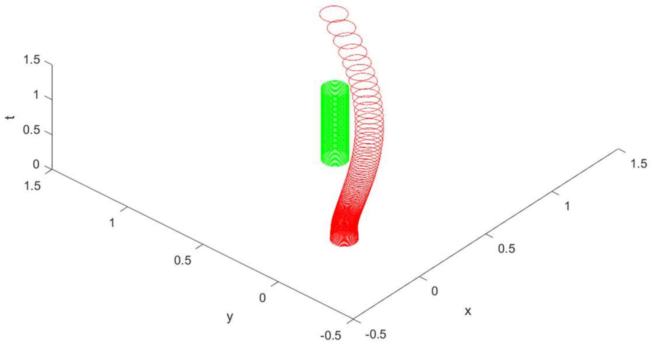
The elliptical tubes of trajectories without regard of the obstacle constraints are shown in Figure 1, and the elliptical tubes of trajectories with regard of the obstacle constraints are shown in Figure 2, where the vertical trajectories tube is the obstacle, and the curved trajectories tube is $E_c[t]$. It can be seen from the simulation results in Figure 1 and Figure 2 that when obstacle constraint is not considered, $E_c[t]$ cannot avoid the obstacle. When considering obstacle constraint, $E_c[t]$ can avoid the obstacle.

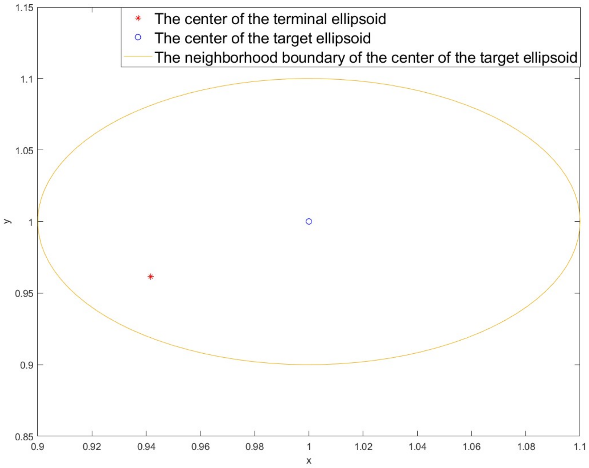
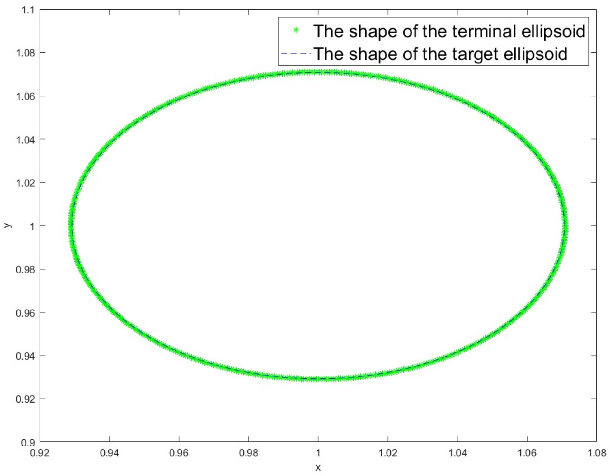
The comparison diagram of the terminal ellipse and the target ellipse without obstacle constraint and with obstacle constraint are given. The simulation results are provided in Supplementary Materials and shown in Figure 3, Figure 4 and Figure 5. In Figure 3, the center of $E_c[t]$ reaches the target set without obstacle constraint. In Figure 4, the center of $E_c[t]$ reaches the target set with obstacle constraint. In Figure 5, the configuration matrix $E_c[t]$ reaches the target set with or without obstacle constraint.

5. Conclusions

This paper studies the collision avoidance problem in formation control and presents a solution to realize collision avoidance based on dynamic programming. By introducing a barrier constraint into the value function, we obtain the optimal controls on the virtual ellipsoid to pass through the obstacle. For the three-dimensional case of a virtual ellipsoid, the method using this article can obtain similar results.

Our work focuses on a situation with static obstacles. This framework is flexible and extensible, and the results of collision avoidance are stable. Meanwhile, several limitations remain to be studied in the future. For example, the current algorithm has not yet achieved parallel computing and still needs to be improved. Additionally, when the obstacle is movable or when actively interfering movement towards the virtual ellipsoid is considered, the target control problem will be converted to a kind of complex game problem which will be studied in the future.

References

- Roman, R.-C.; Precup, R.-E.; Petriu, E.M. Hybrid Data-Driven Fuzzy Active Disturbance Rejection Control for Tower Crane Systems. Eur. J. Control 2021, 58, 373–387. [Google Scholar] [CrossRef]
- Chi, R.; Li, H.; Shen, D.; Hou, Z.; Huang, B. Enhanced P-type Control: Indirect Adaptive Learning from Set-point Updates. IEEE Trans. Automat. Control 2022, 665–669. [Google Scholar] [CrossRef]
- Gustavi, T.; Hu, X.M. Observer-based leader-following formation control using onboard sensor information. IEEE Trans. Robot. 2008, 24, 1457–1462. [Google Scholar] [CrossRef]
- Mariottini, G.L.; Morbidi, F.; Prattichizzo, D.; Valk, N.V.; Michael, N.; Pappas, G.; Daniilidis, K. Vision-based localization for leader-follower formation control. IEEE Trans. Robot. 2009, 25, 1431–1438. [Google Scholar] [CrossRef]
- Chen, X.; Yan, P.; Serrani, A. On input-to-state stability-based design for leader/follower formation control with measurement delays. Int. J. Robust Nonlin. 2013, 23, 1433–1455. [Google Scholar] [CrossRef]
- Panagou, D.; Kumar, V. Cooperative visibility maintenance for leader-follower formations in obstacle environments. IEEE Trans. Robot. 2014, 30, 831–844. [Google Scholar] [CrossRef]
- Kownacki, C. Multi-UAV flight using virtual structure combined with behavioral approach. Acta Mech. Autom. 2016, 10, 92–99. [Google Scholar] [CrossRef]
- Antonelli, G.; Arrichiello, F.; Chiaverini, S. Experiments of formation control with multirobot systems using the null-space-based behavioral control. IEEE. Trans. Control Syst. Technol. 2009, 17, 1173–1182. [Google Scholar] [CrossRef]
- Ren, W.; Beard, R.W. Decentralized scheme for spacecraft formation flying via the virtual structure approach. J. Guid. Control. Dynam. 2004, 27, 73–82. [Google Scholar] [CrossRef]
- Sadowska, A.; den Broek, T.V.; Huijberts, H.; van deWouw, N.; Kostić, D.; Nijmeijer, H. A virtual structure approach to formation control of unicycle mobile robots using mutual coupling. Int. J. Control 2011, 84, 1886–1902. [Google Scholar] [CrossRef]
- Gazi, V. Swarm aggregations using artificial potentials and sliding-mode control. IEEE Trans. Robot. 2005, 21, 1208–1214. [Google Scholar] [CrossRef]
- Mabrouk, M.; McInnes, C. Solving the potential field local minimum problem using internal agent states. Robot. Auton. Syst. 2008, 56, 1050–1060. [Google Scholar] [CrossRef]
- Zhang, J.L.; Yan, J.G.; Zhang, P. Fixed-wing UAV formation control design with collision avoidance based on an improved artificial potential field. IEEE. Access 2018, 6, 78342–78351. [Google Scholar] [CrossRef]
- Xie, L.; Liu, S. Dynamic obstacle-avoiding motion planning for manipulator based on improved artificial potential filed. IET Control Theory A 2018, 35, 1239–1249. [Google Scholar]
- Jiang, A.; Yao, X.; Zhou, J. Research on path planning of real-time obstacle avoidance of mechanical arm based on genetic algorithm. J. Eng. 2018, 16, 1579–1586. [Google Scholar] [CrossRef]
- Li, S.L.; He, J.H.; Ao, H.Y.; Liu, Y.B. Intelligent visibility graph algorithm of Mars aircraft based on pigeon-inspired optimization. Flight. Dyn. 2020, 38, 90–94. [Google Scholar]
- Chen, G.R.; Guo, S.; Wang, J.Z.; Qu, H.B.; Chen, Y.Q.; Hou, B.W. Convex optimization and A-star algorithm combined path planning and obstacle avoidance algorithm. J. Control Decis. 2020, 35, 2907–2914. [Google Scholar]
- Kurzhanski, A.B. Problem of collision avoidance for a team motion with obstacles. Proc. Steklov Inst. Math. 2016, 293, 120–136. [Google Scholar] [CrossRef]
- Kurzhanski, A.B.; Mitchell, I.M.; Araiya, P.V. Optimization techniques for state-constrained control and obstacle problems. J. Optim. Theory Appl. 2006, 128, 499–521. [Google Scholar] [CrossRef][Green Version]
- Kurzhanski, A.B. The problem of measurement feedback control. J. Appl. Math. Mech. 2004, 68, 487–501. [Google Scholar] [CrossRef]
- Komarov, Y.; Kurzhanski, A.B. Minimax-maximin relations for the problem of vector-valued criteria optimization. Dokl. Math. 2020, 101, 259–261. [Google Scholar] [CrossRef]
- Kurzhanski, A.B.; Valyi, I. Ellipsoidal Calculus for Estimation and Control; Springer: Berlin/Heidelberg, Germany, 1997. [Google Scholar]
- Kurzhanski, A.B. On the problem of control for ellipsoidal motions. Proc. Steklov Inst. Math. 2012, 277, 160–169. [Google Scholar] [CrossRef]
- Kurzhanski, A.B. On a team control problem under obstacles. Proc. Steklov Inst. Math. 2015, 51, 128–142. [Google Scholar] [CrossRef]
- Kurzhanski, A.B.; Mesyats, A.I. Optimal control of ellipsoidal motions. Differ. Equ. 2012, 48, 1502–1509. [Google Scholar] [CrossRef]
- Kurzhanski, A.B.; Mesyats, A.I. Control of ellipsoidal trajectories: Theory and numerical results. Comput. Math. Math. Phys. 2014, 54, 418–428. [Google Scholar] [CrossRef]
- Dockner, E.J.; Jorgensen, S.; Long, N.V.; Sorger, G. Differential Games in Economics and Management Science, 1st ed.; Cambridge University Press: Cambridge, UK, 2000. [Google Scholar]