Sizing and Sitting of Battery Energy Storage Systems in Distribution Networks with Transient Stability Consideration

Abstract

In this study, the capacity and location of battery energy storage systems (BESSs) in a distribution network were evaluated to increase the stability and reliability of power systems by applying the proposed transient stability indicators. The search capability of particle swarm optimization (PSO) combined with Pareto optimality in MATLAB R2019b was used to solve multi-objective problems in steady-state conditions, including active power loss, voltage deviation, and total operating cost. The BESS capacity and location were then derived using the Manhattan distance method. Subsequently, the BESS control model was constructed using the commercial software DIgSILENT PowerFactory 2021 to evaluate generator power smoothing and short-term voltage stability index during the transient response and determine the final capacity and location of BESS in distribution networks. Finally, the accuracy of the proposed method was verified by considering the daily load and solar power generation curves using the IEEE 33-bus radial power distribution network.

1. Introduction

With the rise in environmental awareness in recent years and the growing problem of global energy supply, governments around the world are actively developing renewable energy sources. The capacity of renewable energy installations worldwide is increasing rapidly, with solar and wind power being the mainstream. According to the Renewables 2020 Global Energy Status Report, the capacity of renewable energy installations grew by more than 200 GW in 2019. Currently, renewable energy has become an integral part of power generation. The International Renewable Energy Agency (IRENA) [1] analyzed that 260 GW of new renewable energy installations was added globally in 2020, showing a significant increase from the 176 GW of new renewable energy installations in 2019. The increasing number of installations is because renewable energy can be used to improve peak electricity demand and reduce long-distance transmission line losses and transmission line congestions. However, grid integration of numerous renewable energy sources may bring unforeseen problems to the frequency, voltage, and stability of power systems. Some countries have drawn up relevant regulations to improve the impact of grid-connected renewable energy sources; such regulations were compiled in [2]. Moreover, the Institute of Electrical and Electronics Engineers (IEEE) proposed specifications for the grid-connected features, safety considerations, and island operations of distributed energy resources (DERs) at primary or secondary distribution voltage levels in IEEE Std. 1547 [3]. Additionally, Germany introduced VDE-AR-N 4105 as the new standard for low voltage grid-connected features [4]. The application guide is used for the connection of DERs with low voltage levels and capacities equal to or less than 100 kVA. Moreover, China used GB-T 19964 as a standard [5], proposing technical specifications for the integration of solar power into power systems, especially high-voltage solar power systems. Since renewable energy is booming worldwide, it is essential to establish regulations and codes to jointly maintain the power quality, network reliability, voltage stability, and public safety of power systems.

Taiwan has an isolated power system that must be self-sufficient in its power supply. Therefore, an adequate, reliable, and stable power supply is required for economic development. On the other hand, the power gap problem, in addition to the environmental awareness of energy saving and carbon reduction, has been growing in recent years. Hence, developing different types of renewable energy sources is desirable to replace conventional thermal and nuclear electricity generation. However, the increasing proportion of renewable energy holds both advantages and disadvantages for power grids because renewable energy resources exhibit an uncontrollable and intermittent nature. Accordingly, the energy storage system (ESS) is necessarily used to support these problems since it has the energy-time-shifting ability. Therefore, the generated energy can be used at the expected time to compensate for the uncontrollable and intermittent nature of renewable energy. There are four main types of ESS: physical, electromagnetic, phasitrons, and electrochemical energy storage. Among them, the electrochemical energy storage, known as the battery energy storage system (BESS), is typically installed in power grids. BESS has the greatest potential, mainly for balancing power supply and demand [6], improving voltage deviation [7,8], reducing power loss [9,10,11,12], storing power during the off-peak period, and supplying power to the power grid during the peak period [13,14]. BESS is also used as a voltage source or uninterruptible power supply in a microgrid when the utility grid supply or renewable energy source collapses [15]. In conclusion, BESS is beneficial in many applications.

In order to improve the efficiency and reliability of power systems, Naidji et al. proposed the contingency sensitivity index (CSI) method to determine the optimal capacity and most efficient location of an ESS in a modified IEEE 30-bus system. The CSI represented the impact of emergency events on power systems. The total cost (including the investment cost of the storage equipment, voltage deviation, and power loss) was considered the objective function to be minimized in the power system [16]. Moreover, Nick et al. considered the multi-objective problem of achieving an optimal balance between technical and economic objectives, including the cost of voltage deviation, line loss, load supply, and storage system investment, using second-order cone programming (SOCP) to optimize the capacity and location of ESSs in distribution networks [17]. In [18], the authors proposed the optimal size of an installed BESS for storing the electrical energy during the valley load period and supplying it during the peak load period to maximize the operational benefits. Then, Ref. [19] presented various cases of dynamic operations in microgrids according to BESS and photovoltaic (PV) generation systems, including the change in load power, intermittent and unstable operation of the PV sources, on/off-grid operation modes of the microgrid, and discharging and charging states of the BESS. Furthermore, an effective control method was developed to coordinate the operation of distributed ESSs in a distribution network, considering the capacity and state of charge (SoC) of each ESS to accommodate daily operations [20]. Moreover, Jayasekara et al. proposed a suitable method to determine the optimal sizing and sitting of a BESS by minimizing the battery capacity, the number of installations, and maintenance costs. However, the results showed that the sizing and sitting of the BESS were inefficient [21].

Therefore, considering the previous problems, the multi-objective particle swarm optimization (MOPSO) algorithm was used in this study to solve multi-objective problems. The objective functions include active power loss, voltage deviation, and total operating cost, which are minimized using the Manhattan distance method, through which the optimum BESS capacity and location are obtained. Then, the transient response of the BESS in power systems was evaluated using DIgSILENT. After considering each BESS power output, the active power was injected into the system through proportional-integral (PI) and proportional-integral-derivative (PID) control. Thereafter, the IEEE-33 bus test system and BESS control model were constructed for the scenario study. The final results were obtained by generator power smoothing, and the short-term voltage stability index for the BESS capacity and location was derived from the Manhattan distance method. Subsequently, the daily load and solar power generation curves were considered to verify the simulation results. The schematic diagram of the proposed MATLAB and DIgSILENT simulations is shown in Figure 1.

The main contributions of this work are as follows.

• The sizing and sitting of a BESS in distribution networks with connected renewable energy sources were provided by considering the active power loss, voltage deviation, and total operating cost as the objective functions to minimize;
• Generator power smoothing and short-term voltage stability index were considered using the transient response as the selection strategy to determine the final capacity and location of the BESS.

Finally, the rest of the paper is organized as follows: In Section 2, we introduce the network component models by DIgSILENT; in Section 3, we present the objective functions and constraints; in Section 4, we describe the proposed algorithm and solution steps; in Section 5, we illustrate the analytical results and comparisons; and in Section 6, we present our conclusions.

2. Network Component Modeling by DIgSILENT PowerFactory

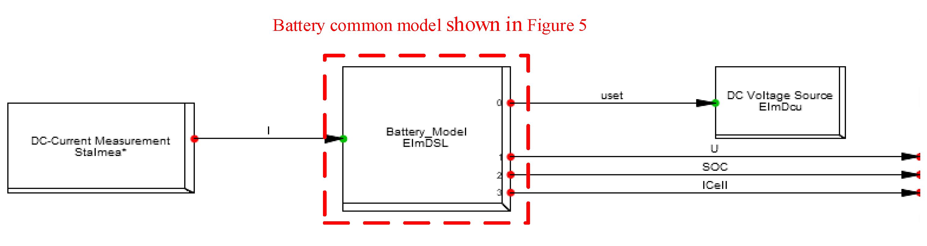
PowerFactory 15.2 is a software developed by DIgSILENT GmbH, independent software and consulting company based in Gomaringen, Germany, that is suitable for power generation, transmission, distribution, and industrial grid analyses. It combines its system modeling capabilities with advanced algorithm concepts. In this study, the DIgSILENT Simulation Language (DSL) model in PowerFactory 15.2 was applied to construct the BESS model, which included battery and smart inverter models. The schematic diagram is shown in Figure 2.

2.1. Battery Model

Lead–acid batteries are often used in DERs because of their advanced and low-cost technology with the longest development history. The electrode is composed mainly of lead (Pb) and oxygen (O), and the sulfuric acid solution is used as the battery electrolyte. The BESS is mainly charged and discharged through the oxidation-reduction reactions at the positive and negative poles of the batteries. In the charge state of a lead–acid battery, the main component in the positive plate is lead dioxide, and the negative plate is Pb. While in the discharge state, the main component in the positive and negative plates is lead sulfate, as shown in Figure 3.

As shown in Figure 2, the DSL is constructed by selecting the network elements and structuring composite and common models. In this study, the composite model of the battery is created using the current signal module (StaImea), common model module (ElmDSL), and network element module (ElmDcu), and its connections are shown in Figure 4. At the same time, the common model of the battery contains the control strategy model and the initial condition definition for the input and output parameters, and its main control framework is illustrated in Figure 5.

2.2. Smart Inverter Model

In recent years, BESSs have been integrated rapidly and heavily into power grids with renewable energy resources. BESSs have a significant impact on system voltage and frequency. In response to this situation, research is being conducted on smart inverters. Smart inverter outputs are generated by pulse-width modulation (PWM) based on a synchronized rotary axis composed of two control loops. In this study, a voltage-source converter was used, assuming that the DC side is an ideal voltage source. The switch is controlled by the current inner-loop method, and the outer loop is controlled by the active and reactive power. The d-axis signal controls the active power, and the q-axis signal controls the reactive power by synchronizing the rotary axis coordinates. Furthermore, the architecture of the voltage source inverter controller is shown in Figure 6.

In an inner-loop control, the three-phase currents and voltages at the output of the converter are captured. The abc components are then converted into αβ0 components using the Clarke transformation, as shown in Equations (1) and (2).

$$\left[\begin{array}{c}{i}_{\alpha }\left(t\right)\\ i_{\beta }\left(t\right)\\ i_0\left(t\right)\end{array}\right]=\frac{2}{3}\left[\begin{array}{ccc}1& -\frac{1}{2}& -\frac{1}{2}\\ 0& \frac{\sqrt{3}}{2}& -\frac{\sqrt{3}}{2}\\ \frac{1}{2}& \frac{1}{2}& \frac{1}{2}\end{array}\right]\left[\begin{array}{c}{i}_a\left(t\right)\\ i_b\left(t\right)\\ i_c\left(t\right)\end{array}\right]$$

(1)

$$\left[\begin{array}{c}{v}_{\alpha }\left(t\right)\\ v_{\beta }\left(t\right)\\ v_0\left(t\right)\end{array}\right]=\frac{2}{3}\left[\begin{array}{ccc}1& -\frac{1}{2}& -\frac{1}{2}\\ 0& \frac{\sqrt{3}}{2}& -\frac{\sqrt{3}}{2}\\ \frac{1}{2}& \frac{1}{2}& \frac{1}{2}\end{array}\right]\left[\begin{array}{c}{v}_a\left(t\right)\\ v_b\left(t\right)\\ v_c\left(t\right)\end{array}\right]$$

(2)

Subsequently, the αβ0 components are transformed into dq0 components using the Park transformation, as shown in Equations (3) and (4).

$$\left[\begin{array}{c}{i}_d\left(t\right)\\ i_q\left(t\right)\\ i_0\left(t\right)\end{array}\right]=\left[\begin{array}{ccc}cos\left(\epsilon \left(t\right)\right)& sin\left(\epsilon \left(t\right)\right)& 0\\ -sin\left(\epsilon \left(t\right)\right)& cos\left(\epsilon \left(t\right)\right)& 1\\ 0& 0& 1\end{array}\right]\left[\begin{array}{c}{i}_{\alpha }\left(t\right)\\ i_{\beta }\left(t\right)\\ i_0\left(t\right)\end{array}\right]$$

(3)

$$\left[\begin{array}{c}{v}_d\left(t\right)\\ v_q\left(t\right)\\ v_0\left(t\right)\end{array}\right]=\left[\begin{array}{ccc}cos\left(\epsilon \left(t\right)\right)& sin\left(\epsilon \left(t\right)\right)& 0\\ -sin\left(\epsilon \left(t\right)\right)& cos\left(\epsilon \left(t\right)\right)& 1\\ 0& 0& 1\end{array}\right]\left[\begin{array}{c}{v}_{\alpha }\left(t\right)\\ v_{\beta }\left(t\right)\\ v_0\left(t\right)\end{array}\right]$$

(4)

In the case of a fixed frequency, $\epsilon$ is calculated using Equation (5), where ${\omega }_0$ is the AC frequency, and ${\epsilon }_0$ is a constant and is the initial phase angle between the αβ0 and dq0 components.

$$\epsilon ={\epsilon }_0+{\omega }_{0}t$$

(5)

Moreover, the active and reactive powers in the three-phase coordinate system are given by Equation (6).

$$\left\{\begin{array}{c}P=\frac{3}{2}{v}_d{i}_{d }\\ Q=-\frac{3}{2}{v}_q{i}_q\end{array}\right.$$

(6)

2.3. BESS Model

The BESS consists of a battery, a smart inverter, a battery management system, and an energy management system. BESS can increase the system voltage, stabilize the system frequency, and improve the transient stability, thus enhancing the reliability of power systems. In this study, the battery was operated in the discharge mode when active power was injected into the power system. The BESS composite model is shown in Figure 7. In the Pf controller, the input is the active power or system frequency, as shown in Figure 8a, whereas, in the QV controller, the input is the reactive power or bus voltage, as shown in Figure 8b. The measurement signal is first calculated by filtering the oscilloscope outputs such that the result is more precise when calculated with the reference value. Subsequently, the error signals are compensated using PID and PI controllers. Finally, the output results are presented as id_ref_in and iq_ref_in, respectively.

3. Problem Formulations

BESS has become an essential component to support energy transitions in many countries, and Taiwan is no exception. BESS is expected to improve power loss and increase the system bus voltage. However, the implementation of a BESS may be expensive. Therefore, it is crucial to consider system responses and cost factors for BESS installation. Accordingly, the objective functions and system constraints of the BESS used in this study are described as follows.

3.1. Control Variables

In order to satisfy the objective function of the planned control variables, the feasible solution interval of the objective function and the restriction condition of the inequality are expressed as

$$\min f_n\left(\mathit{x},\mathit{u}\right), n\in \left\{1,2,\cdots N\right\}$$

(7)

$$\mathrm{subject} \mathrm{to} g_i\left(\mathit{x},\mathit{u}\right)\le 0, i\in \left\{1,2,\cdots I\right\}$$

(8)

$$\mathit{x}\in \mathit{X}$$

(9)

Here, $f_n\left(\mathit{x},\mathit{u}\right)$ is the nth objective function; $g_i\left(\mathit{x},\mathit{u}\right)$ is the ith constraint; x is the control variable; and u is the dependent variable.

This study focused on the design of the capacity and location of a BESS to satisfy the designed objective functions. Therefore, the control variable x and the dependence variable u based on MOPSO can be expressed as Equations (10) and (11), respectively.

$$\mathit{x}={\left[BES{S}_{loc,1},\cdots ,BES{S}_{loc,n},BES{S}_{cap,1},\cdots ,BES{S}_{cap,n}\right]}^T$$

(10)

$$\mathit{u}={\left[V_1,\cdots ,V_i,V_1,\cdots ,V_j,P_{B,1},\cdots ,P_{B,n},P_{loss,1},\cdots P_{loss,n}\right]}^T$$

(11)

$BES{S}_{loc,n}$ is the nth location of the BESS; $BES{S}_{cap,n}$ is the nth capacity of the BESS; $V_i$ and $V_j$ are the voltages at bus-i and bus-j, respectively; $P_{B,n}$ and $P_{loss,n}$ are the nth active power output and the nth active power loss by the BESS, respectively.

3.2. Objective Functions

In this study, the objective functions are (1) active power loss, (2) voltage deviation, and (3) total operating cost.

3.2.1. Active Power Loss

Active power loss is an aspect of the capacity and location optimization problem that cannot be ignored; therefore, the first objective function is defined using Equation (12).

$$\min f_1={\displaystyle \sum }_{i,j\in n}^{N_b}{g}_{ij}\left(V_i{}^2+V_j{}^2-2V_i{V}_{j}cos{\theta }_{ij}\right),$$

(12)

where $N_b$ is the number of buses in the power system; n is the node; $g_{ij}$ is the admittance on branch-$ij$; $V_i$ and $V_j$ are the voltages at bus-i and bus-j, respectively; and ${\theta }_{ij}$ is the voltage phase displacement on branch-$ij$.

3.2.2. Voltage Deviation

Voltage deviation is an important indicator for evaluating safety and power quality [22]; hence, it is considered the second objective function. To evaluate the voltage deviation of bus-$i$, Equation (13) was applied.

$$\min f_2={\displaystyle \sum }_{i=1}^{N_b}{\left(V_i-V_{rated}\right)}^2,$$

(13)

where $N_b$ is the number of buses in the power system; $V_{rated}$ is the nominal voltage at a bus, which is defined as 1.00 p.u.; and $V_i$ is the voltage at bus-i in the power system.

3.2.3. Total Operating Cost

As important as the minimization of active power loss and voltage deviation, the minimization of the total operating cost (TOC) also becomes the objective function, and the cost evaluation was performed using Equation (14) [23].

$$\min f_3={\mathrm{k}}_{\mathrm{b}}·f_G+{\mathrm{k}}_{\mathrm{i}}·f_L,$$

(14)

where ${\mathrm{k}}_{\mathrm{b}}$ is the power generation factor of the BESS and ${\mathrm{k}}_{\mathrm{i}}$ is the loss cost factor.

TOC includes BESS generation cost, as shown in Equation (15), and loss cost, as shown in Equation (16), where $P_B$ is the active power output provided by the BESS; ${\mathrm{a}}_1$, ${\mathrm{a}}_2$, and ${\mathrm{a}}_3$ are quadratic cost coefficients; and $P_{loss}$ is the active power loss obtained by power flow calculations. Furthermore, ${\mathrm{K}}_1$ is the annual load cost; ${\mathrm{K}}_2$ is the price of energy loss; ${\mathrm{L}}_{\mathrm{f}}$ is the loss factor evaluated using Equation (17), where $\mathrm{k}$ and ${\mathrm{l}}_{\mathrm{f}}$ are the loss factor constants.

$$f_G={\mathrm{a}}_1·P_B{}^2+{\mathrm{a}}_2·P_B+{\mathrm{a}}_3$$

(15)

$$f_L=P_{loss}·\left({\mathrm{K}}_1+{\mathrm{K}}_2·{\mathrm{L}}_{\mathrm{f}}·8760\right)$$

(16)

$${\mathrm{L}}_{\mathrm{f}}=\mathrm{k}·{\mathrm{l}}_{\mathrm{f}}+\left(1-\mathrm{k}\right)·{\mathrm{l}}_{\mathrm{f}}{}^2$$

(17)

3.3. Constraints

In the following subsection, we explained the implementation of voltage, capacity, and power flow constraints to comply with the power-system operation standards after connecting the BESS to the grid.

3.3.1. Voltage Constraints

The voltages at all buses shall remain within the allowable range shown in Equation (16).

$$V_{min}\le V_i\le V_{max},$$

(18)

where $V_{min}$ is the lower boundary of the voltage, defined as 0.95 p.u.; $V_{max}$ is the higher boundary of the voltage, defined as 1.05 p.u.; and $V_i$ is the voltage magnitude at bus-$i$.

3.3.2. BESS Technical Constraints

The installation capacity of each BESS depends on its type and operating conditions. The Taiwan Power (Taipower) company classifies BESS capacity according to the voltage level, and the installation capacity shall remain between 100 and 10,000 kW. The operation of the BESS should also be considered in terms of energy constraints. The permissible levels of the BESS are shown in Equations (19) and (20).

$$P_{B,min}\le P_B\le P_{B,max}$$

(19)

$$So{C}_{min}\le SoC\le So{C}_{max}$$

(20)

$P_B$ is the active power output of the BESS; $P_{B,min}$ and $P_{B,max}$ are its boundary limits; and $SoC$ is the battery charging status with $So{C}_{min}$ and $So{C}_{max}$ as the boundary limits.

3.3.3. Branch Power Flow Constraints

The power provided by the BESS grid connection may increase the power flow in transmission lines. In order to avoid line overloading, the power flowing through the transmission lines must be within the allowable thermal limit shown in Equation (21).

$$S_{line}\le \left|S_{max,line}\right|,$$

(21)

where $S_{line}$ is the power flow through the transmission line and $S_{max,line}$ is the related line thermal capacity.

4. Proposed Algorithm

Currently, optimization algorithms are widely used in various fields, such as engineering, applied science, and mathematics. Typically, an optimization algorithm is eminent for its systematic search features with a random search mechanism. An optimization algorithm can avoid convergence into regional best solutions and effectively improve the search performance for global best solutions (Gbest). In recent years, many optimization algorithms have been developed, such as the genetic algorithm (GA) [24], particle swarm algorithm (PSO) [25], and the ant colony algorithm [26].

4.1. Pareto Optimality

Most practical engineering problems have multiple design objectives. Therefore, it is essential to consider multi-objective conditions simultaneously to determine the best solution for each combination of objective designs. When satisfying all design objectives without simplifying any objective function, some feasible solutions in the solution set are superior to others. If no solutions exist superior to a particular solution in all objective functions, then the solution is called a non-dominated solution. The set of all combinations of non-dominated solutions is called the set of Pareto-optimal solutions. In terms of minimization objectives, domination can be expressed as in Equation (22).

$$f_n\left({\mathit{x}}^{\prime }\right)<f_n\left({\mathit{x}}^{″}\right), \forall n\in \left\{1,2,\cdots ,N\right\}$$

(22)

where ${\mathit{x}}^{\prime }$ for all objectives is better than ${\mathit{x}}^{″}$ because ${\mathit{x}}^{\prime }$ is the dominant solution and ${\mathit{x}}^{″}$ is the dominated solution. Thus, a non-dominated solution is obtained when no other solution is found to be better than the dominant solution. Then, all non-dominated solutions in the solution set space can be expressed as in Equation (23), where ${\mathit{x}}_i$ is the ith non-dominated solution.

$$\mathit{P}{\mathit{S}}^A=\left\{{\mathit{x}}_1,{\mathit{x}}_2,\cdots {\mathit{x}}_i\right\}$$

(23)

4.2. Particle Swarm Optimization (PSO)

In 1995, Kennedy and Eberhart proposed a new type of algorithm inspired by the flocks of birds in nature called the particle swarm algorithm (PSO). In the PSO algorithm, the possible solution positions in the solved space are treated as bird movement spaces. The possibility for better solutions during the solution process is gradually improved by transmitting messages from individuals to each other.

In the PSO algorithm, an individual flies at a certain speed in the search space, and the direction and distance of the flight are controlled by particle velocity. According to the flight experience of the individual and group, the flight speed is dynamically adjusted, and the individual gradually moves to a better area of the problem space. The PSO algorithm is initialized for a group of random particles. By following the present best particle, the search position is continuously iterated to determine the best or most efficient solution. In each iteration, each particle is updated after determining the personal best solution (the present best solution of the particle) and Gbest (the present best solution found by the entire population). The velocity increment during the flight process is closely related to the flight experience of the individual and swarm and is limited by the maximum flight speed, as shown in Figure 9.

The MOPSO algorithm, adopted from [27], applies the search capabilities of the PSO algorithm combined with Pareto optimality. A flowchart of the MOPSO algorithm is shown in Figure 10, and the steps of the proposed algorithm are as follows.

Step (1)

Initialize parameters and population: set the number of particle swarms, external archive, number of iterations, and other parameters;

Step (2)

Generate randomly: generate the position and velocity of each particle randomly;

Step (3)

Select fitness: the fitness of each particle is calculated according to the objective function, and the non-dominated solution is obtained from the particle swarms and stored in the external archive;

Step (4)

Select Gbest: start the iteration and select a non-dominant solution as Gbest from the external archive;

Step (5)

Update: use the velocity and position of the particle update formula to obtain the new position and velocity of the particles;

Step (6)

Evaluate the fitness of the particles: evaluate the fitness of each particle based on the objective function;

Step (7)

Select non-dominated solutions: find new non-dominated solutions from the population;

Step (8)

Check the external archive: determine whether the external archive is full or not;

Step (9)

When the external archive is not full, the new non-dominated solution obtained from Step 7 is compared with the non-dominated solution in the external archive. If any solution in the external archive dominates the new solution, it is discarded. Otherwise, if the new solution dominates any solution in the external archive, then the dominated solution in the archive is deleted, and the new solution is stored;

Step (10)

When the external archive is full, the more crowded archives are removed according to the congestion level, and new solutions are deposited.

4.3. Minimum Manhattan Distance Method

In order to find the ideal result, Chiu et al. [28] proposed the minimum Manhattan distance (MMD) to select the final solution among a set of Pareto fronts called multi-criteria decision-making (MCDM). The minimum distance from the normalized ideal vector is called the MMD.

After MOPSO evaluation, many non-dominated solutions in a Pareto front can be obtained, and the minimum value of each objective function is found in the Pareto front. The ideal vector ${\mathit{y}}_{opt}$ can be calculated by normalizing the minimum value of each objective function, as shown in Equation (24).

$${\mathit{y}}_{opt}={\left[\frac{{\rho }_1}{L_1} \frac{{\rho }_2}{L_2} \cdots \frac{{\rho }_N}{L_N}\right]}^{\mathit{T}}$$

(24)

The minimum value of the objective function is then calculated using Equation (25).

$${\rho }_N=\underset{{\mathit{x}}_i\in \mathit{P}{\mathit{S}}^A}{\min }{f}_n\left({\mathit{x}}_i\right),$$

(25)

where ${\rho }_N$ is the minimum value of the Nth objective function in the Pareto front $\mathit{P}{\mathit{S}}^A$ for the set of Pareto optimal solution sets and ${\mathit{x}}_i\in \mathit{P}{\mathit{S}}^A$ is the ith solution in the set of all feasible solutions.

Furthermore, $L_N$ is calculated as the deviation between the maximum and minimum values of each objective function, as shown in Equation (26).

$$L_N=\underset{{\mathit{x}}_i\in \mathit{P}{\mathit{S}}^A}{\max }{f}_n\left({\mathit{x}}_i\right)-\underset{{\mathit{x}}_i\in \mathit{P}{\mathit{S}}^A}{\min }{f}_n\left({\mathit{x}}_i\right)$$

(26)

By using the deviation mentioned above, the vector $\mathit{y}\left({\mathit{x}}_i\right)$ that normalizes all the solutions is represented using Equation (27).

$$\mathit{y}\left({\mathit{x}}_i\right)={\left[\frac{f_1\left({\mathit{x}}_i\right)}{L_1} \frac{f_2\left({\mathit{x}}_i\right)}{L_2} \cdots \frac{f_N\left({\mathit{x}}_i\right)}{L_N}\right]}^T$$

(27)

Thus, the minimum Manhattan distance is the shortest distance from the ideal Pareto front among all the solutions, expressed using Equation (28).

$$MMD=\underset{{\mathit{x}}_i\in \mathit{P}{\mathit{S}}^A}{\min }\left(\mathit{y}\left({\mathit{x}}_i\right)-{\mathit{y}}_{opt}{}_1\right),$$

(28)

where ${\Vert ·\Vert }_1$ is Manhattan norm, also termed as 1-norm.

4.4. Final Solution Selection Index

In the Pareto optimal solution based on the results of the Manhattan distance method, the final capacity and location of the BESS are determined by considering th.

4.4.1. Generator Power Smoothinge Generator Power Smoothing and Short-Term Voltage Stability Index

Solar power can provide additional external generation resources to a power grid and reduce the pressure on power units to supply electricity during the peak period. However, its uncontrollable and intermittent characteristics are problematic. For example, solar power disappears in the evening, and the reduced power generation during this period must be compensated by conventional generators. However, the slow response time of conventional generators may worsen the scheduling difficulty. Therefore, to ensure the safety and stability of the power grid, BESS is particularly important as an ancillary service. In this study, we observed the changes in a conventional generator output power by incorporating BESSs with different capacities and in various locations when the hourly load is increased or decreased, using Equation (29).

$$P_{d,t}=P_{s,t}-P_{e,t}, t\in \left\{1,2,\cdots ,24\right\}$$

(29)

where $P_{d,t}$ is the power deviation of the conventional generators at hour t and $P_{s,t}$ and $P_{e,t}$ are the generator power when the load fluctuates and under normal load conditions, respectively, at hour t.

4.4.2. Short-Term Voltage Stability Index

The root-mean-square voltage-dip severity index (RVSI), implemented from [29], was used to evaluate the transient voltage performance for a detailed evaluation of the voltage characteristics after an accidental event. This study introduces an accidental event as a three-phase short-circuit fault in a power system because this event is the most severe case of a short-circuit fault. Short-circuit faults cause a sudden drop in the system voltage, and the fault current flowing through the conductor causes the temperature to rise, causing overheating and equipment damage. Therefore, it is essential to calculate the RSVI using Equations (30) and (31).

$$RVS{I}_{n,t}={\displaystyle \sum }_{i=1}^{N_b}\left|V_{i,t}-V_{i,t_0}\right|, \forall t\in \left[T_s,T_e\right]$$

(30)

$$RVSI=\frac{1}{N_b}{\displaystyle \sum }_{n=2}^{N_b}RVS{I}_{n,t}$$

(31)

$T_s$ is the fault start time; $T_e$ is the time taken for voltage stabilization after the fault is cleared; $V_{i,t}$ is the voltage magnitude of bus-i at time t; $V_{i,t_0}$ is the voltage magnitude of bus-i at time $t_0$; $t_0$ is the initial time; and $N_b$ is the number of buses.

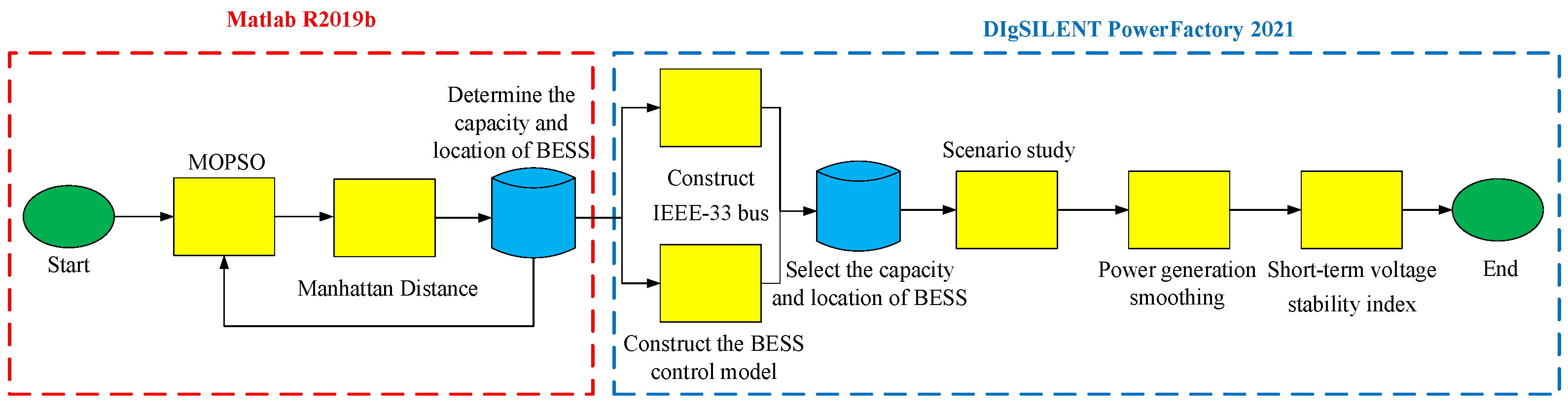
4.5. Proposed Solution Steps

In this study, the MOPSO algorithm was applied to consider the daily load and solar power generation curves in a region in Taiwan. First, the generator output is used as the first indicator. The final BESS capacity and location are then obtained by simulating the short-term voltage stability index. A flowchart of the solution process is shown in Figure 11, and the steps of the proposed solution are as follows.

Step (1)

Build MATLAB benchmark platform: The benchmark-related parameters, such as line impedance, bus voltage magnitude and phase angle, and active and reactive power of the load bus, are built in MATLAB;

Step (2)

Read parameters and mathematical models: The daily load curve and solar power generation curve parameters are incorporated into the benchmark platform. Active power loss, voltage deviation, and cost functions are constructed;

Step (3)

Set constraint condition: Set bus voltage, BESS technical, and branch power-flow constraints;

Step (4)

Initialize: Initialize the state variables and set the particle swarm-related parameters, such as the number of particle swarms, number of iterations, and acceleration factors;

Step (5)

Run the MOPSO algorithm: After the first iteration, the result of each particle is compared with the result of the previous iteration. If the present result is better, then the personal best solution is updated. Moreover, as the global best solution, if the present Gbest is better than the previous iteration result, then Gbest is updated;

Step (6)

Determine the convergence condition: If the convergence condition is satisfied, the output Gbest is obtained; otherwise, repeat Step 5 until the simulation converges;

Step (7)

Run Manhattan distance method: After Gbest is obtained using the MOPSO algorithm, the capacity and location of the BESS are determined using the Manhattan distance method;

Step (8)

Build the DIgSILENT benchmark platform: The benchmark and BESS components, such as generators, loads, transformers, inverters, and batteries, are built in DIgSILENT;

Step (9)

Set models and parameters: Daily load and solar power generation curves are inserted into smart inverter and battery control models;

Step (10)

Select the best neighboring solutions: Select five groups of BESS capacities and locations from the solutions obtained in Step 7;

Step (11)

First transient screening: Set the output from Step 10 into the DIgSILENT. First, generator power smoothing is evaluated when the load changes, then three sets with better BESS capacities and positions are selected;

Step (12)

Second transient screening: Set the output from Step 11 into the DIgSILENT. In the event of a three-phase short-circuit fault at each bus in the power system, the final BESS capacity and location are selected by considering the short-term voltage stability index.

5. Simulation Results

5.1. Sample System

In this study, the IEEE 33-bus system was used as a benchmark to verify the effectiveness of the proposed method. The test system consisted of 33 buses, 32 branches, and 32 loads. Furthermore, the rated voltage of the power system was 12.66 kV. The short-circuit capacity was 100 MVA, and the total real power and reactive power loads were 3.715 MW and 2.3 MVAR, respectively [28]. The single-line diagram of the network system is shown in Figure 12. In addition, a solar power generation system was installed in the test system. Therefore, the solar power generation and load models on each bus were considered with the relevant data provided by Taipower. Finally, the simulation was performed in MATLAB R2019b and DIgSILENT PowerFactory 2021 using a computer with an Intel^® Core(TM)i7-4770 CPU @3.940 GHz, RAM 16 GB, and Windows 10 Pro-64-bit operating system.

5.1.1. Solar Power Generation Model

The hourly solar power generation output can be obtained using Equation (32).

$$P_{PV,t}=P_{PV}·{\mu }_t,$$

(32)

where $P_{PV,t}$ is the solar power generation at hour t, $P_{PV}$ is the rated solar power defined as 1 MW, and ${\mu }_t$ is the coefficient of power generation at hour t [30]. Because solar power exists from 6 a.m. to 7 p.m. and there is no sunshine for the rest of the day, the hourly generation coefficient is calculated, as shown in

Table 1. Hourly power generation coefficient.

Time, Hour	Power Generation Coefficient	Time, Hour	Power Generation Coefficient	Time, Hour	Power Generation Coefficient
0–1	0	8–9	0.39	16–17	0.3448
1–2	0	9–10	0.6223	17–18	0.09206
2–3	0	10–11	0.7923	18–19	0.001702
3–4	0	11–12	0.9214	19–20	0
4–5	0	12–13	1	20–21	0
5–6	0	13–14	0.9612	21–22	0
6–7	0.00842	14–15	0.8576	22–23	0
7–8	0.1425	15–16	0.6394	23–24	0

. The daily solar power generation output, based on the hourly coefficient, is then shown in Figure 13.

5.1.2. Load Model

The hourly load can be obtained using Equation (33).

$$P_{n,t}=P_n·{\delta }_t,$$

(33)

where $P_{n,t}$ is the load demand of the nth bus at time t, $P_n$ is the rated load demand, and ${\delta }_t$ is the load coefficient at time t. As shown in

Table 2. Hourly load coefficient.

Time, Hour	Load Coefficient	Time, Hour	Load Coefficient	Time, Hour	Load Coefficient
0–1	0.7586	8–9	0.9053	16–17	0.9872
1–2	0.7274	9–10	0.9633	17–18	0.9882
2–3	0.7029	10–11	0.9850	18–19	1
3–4	0.6880	11–12	0.9921	19–20	0.9827
4–5	0.6864	12–13	0.9343	20–21	0.9614
5–6	0.6940	13–14	0.9616	21–22	0.93375
6–7	0.7416	14–15	0.9759	22–23	0.8850
7–8	0.7962	15–16	0.9793	23–24	0.8360

, the load coefficient gradually increased after 9 a.m. because the demand load continued to increase and gradually decreased at 11 p.m. as the demand load diminished. The daily load curve is shown in Figure 14.

5.2. Setting Parameters

The objective functions used in this study are the active power loss, voltage deviation, and total operating cost. They are minimized by applying the search capability of PSO combined with Pareto optimality. The parameters of the MOPSO used in this study are listed in

Table 3. Parameters of the proposed MOPSO algorithm.

Item	Parameters
Number of iterations	100
Population size	20
Number of objectives	3
Number of constraints	4
Size of external archive	100
Number of divisions	30

, and the related parameters in the multi-objective function are listed in

Table 4. Parameters related to objective functions of the proposed MOPSO algorithm.

Item	Feasible Ranges of Parameters
${\mathrm{a}}_1$	0
${\mathrm{a}}_2$	20
${\mathrm{a}}_3$	0.25
${\mathrm{K}}_1$	57.6923$/kW
${\mathrm{K}}_2$	0.00961538$/kW
k	0.2
${\mathrm{l}}_{\mathrm{f}}$	0.47
${\mathrm{k}}_{\mathrm{i}}$	0.07
${\mathrm{k}}_{\mathrm{b}}$	5
Capacity for BESS	100–500 kW
Location for BESS	2–33

. The simulations are carried out for one-BESS connection (case 1) and two-BESS connection (case 2).

5.3. One BESS Case Study

The final capacity and location of the BESS were derived based on the hourly load and solar power generation results. The hourly power generation and RVSI values are presented in

Table 5. Final capacity and location of BESS per hour (one BESS connection).

Time, Hour	Capacity, kW	Location	Power Generation, MW	RVSI, p.u.
0–1	419	33	0.090	8.817
1–2	424	33	0.065	10.490
2–3	409	33	0.063	9.742
3–4	386	33	0.062	9.834
4–5	397	33	0.061	10.367
5–6	397	33	0.062	9.924
6–7	409	33	0.066	9.317
7–8	394	33	0.071	9.542
8–9	319	31	0.078	11.452
9–10	330	29	0.083	10.977
10–11	340	14	0.087	7.588
11–12	325	17	0.089	7.584
12–13	301	14	0.082	8.233
13–14	329	17	0.088	5.146
14–15	322	15	0.087	7.254
15–16	357	30	0.085	10.247
16–17	422	32	0.087	9.784
17–18	351	33	0.089	9.807
18–19	354	33	0.090	9.751
19–20	335	33	0.088	10.088
20–21	331	33	0.086	9.095
21–22	352	33	0.084	10.413
22–23	354	33	0.079	9.983
23–24	344	33	0.075	9.698

. During the period 1–7 a.m., the change in power generation was relatively small. Although the power generation is better between 1 and 6 a.m. than between 6 and 7 a.m., the difference is insignificant. RVSI was considered because failure is an abnormal phenomenon. However, RVSI values were better for the rest of the time, and the power generation changed more. Moreover, since the period 6–7 a.m. has a better RVSI than the period 1–6 a.m., the final capacity and location of the BESS were obtained as 409 kW on bus 33 between 6 and 7 a.m.

By considering the period 6–7 a.m., the five best neighboring solutions were obtained using the Manhattan distance method and shown in

Table 6. Best five neighboring solutions obtained by the Manhattan distance method (one BESS connection).

MMD	Power Loss, MW	Voltage Deviation, p.u.	Cost, $	Power Generation, MW	RVSI, p.u.	Capacity, kW	Location
0.7886	0.1714	1.54 × 10−3	40,902	0.06701	10.241	417	31
0.7890	0.1717	1.56 × 10−3	40,502	0.06742	9.6534	405	33
0.7904	0.1720	1.58 × 10−3	40,102	0.06638	9.3171	409	33
0.7908	0.1708	1.50 × 10−3	41,702	0.06820		424	31
0.7960	0.1703	1.46 × 10−3	42,402	0.06832		401	32

. If the result was chosen considering only the shortest distance, which is 0.7886, then the 417 kW BESS on bus 31 was selected. However, by using the strategy proposed in this paper, it was found that this MMD result may not be the best. Therefore, the five best neighboring solutions are necessary to evaluate the generator output and RVSI. Thus, the result with better generator output and RVSI was chosen, which offers the optimum BESS capacity as 409 kW on bus 33.

Assume that a three-phase short-circuit fault occurs in a bus. Observing bus 33, where solar power is generated, if a 417 kW BESS on bus 31 is installed, the voltage drops to 0.6791 p.u., as shown in Figure 15a. Otherwise, if a 409 kW BESS on bus 33 is installed, the voltage becomes 0.7101 p.u., as shown in Figure 15b. In addition, in terms of the RVSI indicator, the 409 kW BESS on bus 33 performs better than the 417 kW BESS on bus 31.

Based on the results of the MOPSO algorithm, the proposed method combined with the Manhattan distance method chooses a 409 kW BESS on bus 33. A comparison of its results with those obtained using the pure PSO algorithm, which is 111 kW BESS on bus 28, is shown in

Table 7. Comparison of the results of MOPSO algorithm and PSO algorithm (one BESS connection).

Algorithm	Power Loss, MW	Voltage Deviation, p.u.	Cost, $	Power Generation, MW	RVSI, p.u.	Capacity, kW	Location
MOPSO	0.1720	1.58 × 10−3	40,102	0.06638	9.3171	409	33
PSO	0.1836	2.42 × 10−3	26,802	0.07254	11.582	268	27

. The MOPSO algorithm outperforms the PSO algorithm in each index, highlighting the effectiveness of the MOPSO algorithm.

Furthermore, the comparisons of the proposed strategy with the MMD results in terms of the generator output and RVSI are shown in Figure 16a,b, respectively. For the generator output, the result from the proposed method is slightly higher than the MMD solution at 6 p.m. The generator output is 0.000016 MW more than the MMD solution, which is insignificant. At 12 p.m., the results of the proposed method allow the unit to produce 0.001976 MW less than the MMD solution. Whereas, for the rest of the time, it is either equal to or lower than the MMD solution. Obviously, the proposed method can determine a solution similar to or even better than MMD in the generator output index. However, for the RVSI, solutions equal to the MMD are found at 2, 8, and 9 p.m. For the rest of the time, a better solution than MMD can be found. For example, at 3 a.m., the proposed method results in an RVSI that allows a total average voltage solution below the MMD of 2.463 p.u. The results demonstrate the effectiveness of the proposed strategy.

5.4. Two BESSs Case Study

When connecting two BESSs, the final hourly BESS capacity and location are derived based on the hourly load and solar power generation results. The hourly power generation and RVSI values are listed in

Table 8. Final capacity and location of BESS per hour (two BESSs connections).

Time, Hour	Capacity, kW	Location	Power Generation, MW	RVSI, p.u.
0–1	477 176	33 16	0.056	8.0737
1–2	465 178	33 16	0.054	8.847
2–3	453 237	33 14	0.051	5.895
3–4	458 100	32 14	0.050	7.912
4–5	410 171	33 15	0.051	7.645
5–6	500 191	33 16	0.052	7.017
6–7	415 100	32 17	0.056	8.214
7–8	346 272	32 14	0.058	7.125
8–9	317 330	32 16	0.066	6.018
9–10	326 269	31 15	0.070	7.231
10–11	234 323	31 15	0.071	6.708
11–12	120 295	32 16	0.073	7.905
12–13	315 183	18 9	0.074	7.264
13–14	194 300	30 16	0.069	8.342
14–15	108 495	29 14	0.069	6.780
15–16	292 321	33 15	0.072	7.582
16–17	351 330	32 15	0.072	7.108
17–18	456 244	33 16	0.073	6.710
18–19	500 216	33 15	0.074	6.357
19–20	500 165	33 13	0.072	7.733
20–21	453 174	33 16	0.072	8.114
21–22	465 189	33 31	0.077	6.393
22–23	500 160	33 14	0.065	6.092
23–24	456 188	33 14	0.061	6.833

. Between 0 and 8 a.m., the power generation change is relatively small. After considering the RVSI, it was found that the best RVSI is between 2 and 3 a.m., even though the power generation between 3 and 4 a.m. is better. Therefore, the final solution, 453 kW BESS on bus 33 and 237 kW BESS on bus 14, was found between 2 and 3 a.m.

Because the final solution is between 2 and 3 a.m., the five best neighboring solutions were obtained using the Manhattan distance method. The results are shown in

Table 9. Best five neighboring solutions obtained by the Manhattan distance method (two BESSs connections).

MMD	Power Loss, MW	Voltage Deviation, p.u.	Cost, $	Power Generation, MW	RVSI, p.u.	Capacity, kW	Location
0.6876	0.1447	8.764 × 10−4	59,002	0.05383	7.8523	463 127	33 15
0.6882	0.1406	10.66 × 10−4	60,602	0.05445		417 189	32 17
0.6956	0.1458	7.697 × 10−4	60,102	0.05380	8.4645	500 100	33 14
0.6991	0.1459	11.02 × 10−4	55,002	0.05521		404 146	33 18
0.6992	0.1360	7.65 × 10−4	60,002	0.05141	5.8953	453 237	33 14

. For the case of connecting two BESSs, if the MMD solution is chosen considering the shortest distance, which is 0.6876, then the selected combination of the two BESSs is 463 kW BESS on bus 33 and 127 kW BESS on bus 15. However, after evaluating the generator output and RVSI, it is evident that this MMD solution may not be the best because even though it results in higher generator output, it does not give the best RVSI. Then, a combination of 453 kW BESS on bus 33 and 237 kW BESS on bus 14 was selected as the final solution because the result is still within the acceptable limits, even though it is slightly more expensive.

Assume that a three-phase short-circuit fault occurs in a bus. By observing bus 33, it can be shown that using a combination of 463 kW BESS on bus 33 and 127 kW BESS on bus 15 adjusts the voltage to 0.7148 p.u., as shown in Figure 17a. However, when a combination of 453 kW BESS on bus 33 and 237 kW BESS on bus 14 is installed, the voltage is adjusted to 0.7887 p.u., as shown in Figure 17b. It is proven that when the same fault occurs, installing one more BESS can reduce the voltage amplitude during the fault.

Based on the results of the MOPSO algorithm, the proposed method combined with the Manhattan distance method chooses a combination of 453 kW BESS on bus 33 and 237 kW BESS on bus 14. This result was then compared with the results of the pure PSO algorithm, which chooses a combination of 100 kW BESS on bus 32 and 119 kW BESS on bus 16. Subsequently, the comparison of the results is shown in

Table 10. Comparison of the results of MOPSO algorithm and PSO algorithm (two BESSs connection).

Algorithm	Power Loss, MW	Voltage Deviation, p.u.	Cost, $	Power Generation, MW	RVSI, p.u.	Capacity, kW	Location
MOPSO	0.1360	7.65 × 10−4	60,002	0.05141	5.8953	453 237	33 14
PSO	0.1756	3.12 × 10−3	21,902	0.06543	10.842	100 119	32 16

. The results of the MOPSO algorithm show that regardless of whether one BESS or two BESSs are connected, the search results are better than those of the PSO algorithm.

Finally, Figure 18a,b show a comparison between the proposed strategy and MMD solution in terms of generator output and RVSI, respectively. For the generator output, the results of the proposed method are equal to or lower than the solution of the MMD at all times. For example, at 1 a.m., 12 p.m., and 2 p.m., the results of the proposed method are similar to those of the MMD solution, and at 1 p.m., it is possible to make the unit output 0.0046 MW less than the MMD solution. The proposed method can determine a solution similar to or even better than MMD in the generator output index. However, for RVSI, a solution equal to the MMD was found at 1 a.m. For the rest of the time, a better solution than MMD can be found. For example, at 3 a.m., the proposed method results in an RVSI that allows a total average voltage solution below the MMD of 2.5693 p.u. The results show that implementing two BESSs is better than implementing one BESS. However, the proposed strategy still outperforms the MMD solutions in terms of both generator output and RVSI, regardless of whether the power system is connected with one BESS or two BESSs.

6. Conclusions

In this study, the capacity and location of BESSs in a distribution network were evaluated using the proposed evaluation indices during the transient response. In order to evaluate the multi-objective problem, the MOPSO algorithm was applied to minimize active power loss, voltage deviation, and total operating cost. Moreover, DIgSILENT was used to build the BESS model and the control strategy. Furthermore, to investigate the performance of the proposed strategy, the proposed method was compared with the MMD and PSO algorithm results. In case studies with one BESS and two BESSs, the results demonstrate the superior performance of the proposed strategy. In addition, in terms of generator output power smoothing and RVSI, the simulation results show that the proposed strategy outperforms the MMD results with better search capability in terms of both the transient response indices. Subsequently, the proposed strategy was verified using the IEEE 33-bus system, demonstrating the excellent performance of the proposed strategy.

References

1. Mengi-Dinçer, H.; Ediger, V.; Yesevi, Ç. Evaluating the international renewable energy agency through the lens of social constructivism. Renew. Sustain. Energy Rev. 2021, 152, 111705. [Google Scholar] [CrossRef]
2. Rebollal, D.; Carpintero-Rentería, M.; Santos-Martín, D.; Chinchilla, M. Microgrid and distributed energy resources standards and guidelines review: Grid connection and operation technical requirements. Energies 2021, 14, 523. [Google Scholar] [CrossRef]
3. Photovoltaics, D.G.; Storage, E. IEEE standard for interconnection and interoperability of distributed energy resources with associated electric power systems interfaces. IEEE Std. 2018, 1547–2018. [Google Scholar] [CrossRef]
4. Bae, Y.; Vu, T.-K.; Kim, R.-Y. Implemental control strategy for grid stabilization of grid-connected pv system based on german grid code in symmetrical low-to-medium voltage network. IEEE Trans. Energy Convers. 2013, 28, 619–631. [Google Scholar] [CrossRef]
5. Wu, Y.-K.; Lin, J.-H.; Lin, H.-J. Standards and guidelines for grid-connected photovoltaic generation systems: A review and comparison. IEEE Trans. Ind. Appl. 2017, 53, 3205–3216. [Google Scholar] [CrossRef]
6. Laugs, G.A.; Benders, R.M.; Moll, H.C. Balancing responsibilities: Effects of growth of variable renewable energy, storage, and undue grid interaction. Energy Policy 2020, 139, 111203. [Google Scholar] [CrossRef]
7. Krata, J.; Saha, T.K. Real-time coordinated voltage support with battery energy storage in a distribution grid equipped with medium-scale pv generation. IEEE Trans. Smart Grid 2018, 10, 3486–3497. [Google Scholar] [CrossRef]
8. Zhang, Y.; Meng, K.; Luo, F.; Yang, H.; Zhu, J.; Dong, Z.Y. Multi-agent-based voltage regulation scheme for high photovoltaic penetrated active distribution networks using battery energy storage systems. IEEE Access 2019, 8, 7323–7333. [Google Scholar] [CrossRef]
9. Alzahrani, A.; Alharthi, H.; Khalid, M. Minimization of power losses through optimal battery placement in a distributed network with high penetration of photovoltaics. Energies 2019, 13, 140. [Google Scholar] [CrossRef]
10. Wong, L.A.; Ramachandaramurthy, V.K.; Walker, S.L.; Taylor, P.; Sanjari, M.J. Optimal placement and sizing of battery energy storage system for losses reduction using whale optimization algorithm. J. Energy Storage 2019, 26, 100892. [Google Scholar] [CrossRef]
11. Costa, J.A.d.; Castelo Branco, D.A.; Pimentel Filho, M.C.; Medeiros Júnior, M.F.d.; Silva, N.F.d. Optimal sizing of photovoltaic generation in radial distribution systems using lagrange multipliers. Energies 2019, 12, 1728. [Google Scholar] [CrossRef]
12. Nor, N.M.; Ali, A.; Ibrahim, T.; Romlie, M.F. Battery storage for the utility-scale distributed photovoltaic generations. IEEE Access 2017, 6, 1137–1154. [Google Scholar] [CrossRef]
13. Zhang, Y.; Campana, P.E.; Lundblad, A.; Yan, J. Comparative study of hydrogen storage and battery storage in grid connected photovoltaic system: Storage sizing and rule-based operation. Appl. Energy 2017, 201, 397–411. [Google Scholar] [CrossRef]
14. Sardi, J.; Mithulananthan, N.; Gallagher, M.; Hung, D.Q. Multiple community energy storage planning in distribution networks using a cost-benefit analysis. Appl. Energy 2017, 190, 453–463. [Google Scholar] [CrossRef]
15. Ganesan, S.; Subramaniam, U.; Ghodke, A.A.; Elavarasan, R.M.; Raju, K.; Bhaskar, M.S. Investigation on sizing of voltage source for a battery energy storage system in microgrid with renewable energy sources. IEEE Access 2020, 8, 188861–188874. [Google Scholar] [CrossRef]
16. Naidji, I.; Smida, M.B.; Khalgui, M.; Bachir, A.; Li, Z.; Wu, N. Efficient allocation strategy of energy storage systems in power grids considering contingencies. IEEE Access 2019, 7, 186378–186392. [Google Scholar] [CrossRef]
17. Nick, M.; Cherkaoui, R.; Paolone, M. Optimal allocation of dispersed energy storage systems in active distribution networks for energy balance and grid support. IEEE Trans. Power Syst. 2014, 29, 2300–2310. [Google Scholar] [CrossRef]
18. Liu, J.; Chen, Z.; Xiang, Y. Exploring economic criteria for energy storage system sizing. Energies 2019, 12, 2312. [Google Scholar] [CrossRef]
19. Pham, T.T.; Kuo, T.-C.; Bui, D.M. Reliability evaluation of an aggregate battery energy storage system in microgrids under dynamic operation. Int. J. Electr. Power Energy Syst. 2020, 118, 105786. [Google Scholar] [CrossRef]
20. Wang, Y.; Tan, K.; Peng, X.Y.; So, P.L. Coordinated control of distributed energy-storage systems for voltage regulation in distribution networks. IEEE Trans. Power Deliv. 2015, 31, 1132–1141. [Google Scholar] [CrossRef]
21. Jayasekara, N.; Masoum, M.A.; Wolfs, P.J. Optimal operation of distributed energy storage systems to improve distribution network load and generation hosting capability. IEEE Trans. Sustain. Energy 2015, 7, 250–261. [Google Scholar] [CrossRef]
22. Nayeripour, M.; Mahboubi-Moghaddam, E.; Aghaei, J.; Azizi-Vahed, A. Multi-objective placement and sizing of dgs in distribution networks ensuring transient stability using hybrid evolutionary algorithm. Renew. Sustain. Energy Rev. 2013, 25, 759–767. [Google Scholar] [CrossRef]
23. Balu, K.; Mukherjee, V. Optimal siting and sizing of distributed generation in radial distribution system using a novel student psychology-based optimization algorithm. Neural Comput. Appl. 2021, 33, 15639–15667. [Google Scholar] [CrossRef]
24. Mirjalili, S. Genetic algorithm. In Evolutionary Algorithms and Neural Networks; Springer: Beilin/Heideburg, Germany, 2019; pp. 43–55. [Google Scholar]
25. Jiang, J.-J.; Wei, W.-X.; Shao, W.-L.; Liang, Y.-F.; Qu, Y.-Y. Research on large-scale bi-level particle swarm optimization algorithm. IEEE Access 2021, 9, 56364–56375. [Google Scholar] [CrossRef]
26. Yue, L.; Chen, H. Unmanned vehicle path planning using a novel ant colony algorithm. EURASIP J. Wirel. Commun. Netw. 2019, 2019, 1–9. [Google Scholar] [CrossRef]
27. Shen, Y.; Ge, G. Multi-objective particle swarm optimization based on fuzzy optimality. IEEE Access 2019, 7, 101513–101526. [Google Scholar] [CrossRef]
28. Chiu, W.-Y.; Yen, G.G.; Juan, T.-K. Minimum manhattan distance approach to multiple criteria decision making in multi-objective optimization problems. IEEE Trans. Evol. Comput. 2016, 20, 972–985. [Google Scholar] [CrossRef]
29. Chi, Y.; Xu, Y. Multi-objective robust tuning of statcom controller parameters for stability enhancement of stochastic wind-penetrated power systems. IET Gener. Transm. Distrib. 2020, 14, 4805–4814. [Google Scholar] [CrossRef]
30. Mahmud, K.; Azam, S.; Karim, A.; Zobaed, S.; Shanmugam, B.; Mathur, D. Machine learning based pv power generation forecasting in alice springs. IEEE Access 2021, 9, 46117–46128. [Google Scholar] [CrossRef]
Figure 1. Schematic diagram of the proposed MATLAB and DIgSILENT simulations.
Mathematics 10 03420 g001
Figure 2. Schematic diagram of DSL model language.
Mathematics 10 03420 g002
Figure 3. Schematic diagram of a lead–acid battery.
Mathematics 10 03420 g003
Figure 4. Composite model of the battery.
Mathematics 10 03420 g004
Figure 5. Common model of the battery.
Mathematics 10 03420 g005
Figure 6. Voltage-source converter controller architecture.
Mathematics 10 03420 g006
Figure 7. Composite model diagram of BESS.
Mathematics 10 03420 g007
Figure 8. Common model diagram of BESS with (a) Pf controller; (b) QV controller.
Mathematics 10 03420 g008
Figure 9. Principle of particle swarm motion.
Mathematics 10 03420 g009
Figure 10. Flowchart of the proposed MOPSO algorithm.
Mathematics 10 03420 g010
Figure 11. Flowchart of the proposed solution.
Mathematics 10 03420 g011
Figure 12. Single-line diagram of IEEE 33-bus system.
Mathematics 10 03420 g012
Figure 13. Daily solar power generation curve.
Mathematics 10 03420 g013
Figure 14. Daily load curve.
Mathematics 10 03420 g014
Figure 15. Fault conditions: (a) 417 kW capacity at bus 31 (b) 409 kW capacity at bus 33.
Mathematics 10 03420 g015
Figure 16. One BESS case study: (a) generator output; (b) RVSI.
Mathematics 10 03420 g016
Figure 17. Fault conditions: (a) 463 kW capacity at bus 33 and 127 kW capacity at bus 15; (b) 453 kW capacity at bus 32 and 237 kW capacity at bus 14.
Mathematics 10 03420 g017
Figure 18. Two BESSs case study: (a) generator output; (b) RVSI.
Mathematics 10 03420 g018aMathematics 10 03420 g018b