The Generalized Exponential Extended Exponentiated Family of Distributions: Theory, Properties, and Applications

Abstract

Here, we propose a new generalized exponential extended exponentiated (NGE3) family of distributions. Some statistical properties of proposed family are gained. The most extreme probability method, maximum likelihood (ML), is utilized for parameter estimation. We explore an exceptional model called NGE3-Exponential (NGE3E). NGE3E is estimated with ML, and the performance of estimators is demonstrated by utilizing a simulation. Moreover, two applications are given to show the significance and adaptability of the proposed model in comparison to some generalized models (GMs).

1. Introduction

We propose a generalized and univariate family of distributions (FoDs) with an exponential random variable (r.v.). Exponential distribution (ED) is a popular continuous probability model that has most extensively been applied in various fields as a life testing model (Lemonte, 2013) [1]. The popularity of ED may be due to the simplicity of its cumulative distribution function (cdf). In addition, the failure rate function (FRF) of ED has a constant shape. Several contemporary classes of distributions have been developed over the last couple of years grounded in the straightforward ED to submit lifetime models that can oblige useful applications where FRFs are decreasing, increasing, bathtub (BT), and upside-down BT (UDBT) shapes since ED does not give a reasonable fit in such circumstances. To increase the flexibility of ED, Adamidis and Loukas (1998) attempted exponential geometric (EG) distribution with decreasing FRF [2]; Gupta and Kundu (2001), the exponentiated ED as extension of the ED that can fit data with decreasing and increasing FRFs [3]; Gupta and Kundu (1999) [4], the generalized ED (GED) having three parameters as an appropriate substitute to the log normal, Weibull, and gamma distributions with increasing and decreasing FRFs. Gupta and Kundu (2007) [5], the GED has a shape of falling, rising, and constant FRFs, so it has not had the ability to fit in with data that have the nonmonotonous failure shape of the UDBT and BT. For more details on the applications and extensions of the exponential distribution, we refer to Balakrishnan (2019) [6] and Johnson et al. (2019) [7]. See also Hussain et al. (2022) [8] and Martínez-Flórez et al. (2020) [9].

Furthermore, for continuous distributions, Alzaatreh et al. (2013) [10] presented the idea of transformed–transformer (T–X) FoDs (TXFoDs). Let $v\left(z\right)$ be the probability density function (pdf) of r.v. Z, where $Z\in [a_1,a_2]$, $-\infty \le a_1<a_2<\infty$, and let $U\left[F\right(x\left)\right]$⤏ be the $F\left(x\right)$ of r.v., X, satisfying the constrains specified below:

1.

$U\left[F\left(x\right)\right]\in [a_1,a_2]$, is differentiable and increases monotonically.

2.

$$U\left[F\left(x\right)\right]\to \left\{\begin{array}{cc}{a}_1\hfill & \mathrm{as}x\to -\infty \hfill \\ a_2\hfill & \mathrm{as}x\to +\infty \hfill \end{array}\right.$$

The cdf of TXFoDs is

$$G\left(x\right)={\int }_{a_1}^{U\left[F\right(x\left)\right]}v\left(z\right)\mathrm{d}z,x\in \mathcal{R},$$

(1)

The corresponding pdf of (1) is

$$g\left(x\right)=v\left\{U\left[F\right(x\left)\right]\right\}\left\{\frac{\partial }{\partial x}U\left[F\left(x\right)\right]\right\}.$$

(2)

Taking the idea from (1), we developed new flexible FoDs called a new generalized exponential extended exponentiated-G (NGE3-G) family (NGE3GF). Let r.v. Z follow the ED with scale parameter $\lambda >0$ and cdf as

$$V\left(z\right)=1-e^{-\lambda z},z\ge 0,$$

(3)

The pdf related to (3) is

$$v\left(z\right)=\lambda e^{-\lambda z},z>0.$$

(4)

Setting $U\left[F\left(x\right)\right]=-log\left\{\frac{\overline{\theta }+\theta \overline{F}{(x;\xi )}^a}{1-log\overline{F}{(x;\xi )}^a}\right\}$ in (1), when $v\left(z\right)$∼ (4), we define the cdf of NGE3GF as

$$\begin{array}{cc}\hfill G(x;\theta ,a,\lambda ,\xi )& =\lambda {\int }_0^{-log\left\{\frac{\overline{\theta }+\theta \overline{F}{(x;\xi )}^a}{1-log\overline{F}{(x;\xi )}^a}\right\}}{e}^{-\lambda z}\mathrm{d}z,\hfill \\ \hfill & =1-{\left\{\frac{\overline{\theta }+\theta \overline{F}{(x;\xi )}^a}{1-log\overline{F}{(x;\xi )}^a}\right\}}^{\lambda },\theta ,a,\lambda >0,x\in \mathcal{R}.\hfill \end{array}$$

(5)

where $\overline{\theta }=1-\theta$, $\overline{F}{(x;\xi )}^a=1-F{(x;\xi )}^a$ and $F(x;\xi )$ or we can simply write $F\left(x\right)$ is baseline (BL) cdf of parameter $\xi$.

The main motivation for (5) follows from NGE3GF succeeding in fitting lifetime data as a competitive model (CM) to widely applied classes.

NGE3GF has a pdf as follows:

$$\begin{array}{cc}\hfill g(x;\theta ,a,\lambda ,\xi )=& \frac{a\lambda f(x;\xi )F{(x;\xi )}^{a-1}}{\overline{F}{(x;\xi )}^a}\frac{{\{\overline{\theta }+\theta \overline{F}{(x;\xi )}^a\}}^{\lambda -1}}{{\{1-log\overline{F}{(x;\xi )}^a\}}^{\lambda +1}}\hfill \\ & \times [\theta \overline{F}{(x;\xi )}^a\{1-log\overline{F}{(x;\xi )}^a\}+\{\overline{\theta }+\theta \overline{F}{(x;\xi )}^a\}].\hfill \end{array}$$

(6)

The paper is organized as follows. We characterize the NGE3GF with its reliability analysis and a convenient linear representation of the pdf and cdf in Section 1. In Section 2, several of its statistical properties are determined. NGE3GF parameters are estimated in Section 3. In Section 4, a special model viz. NGE3-Exponential distribution is discussed. A simulation study, the estimation of the parameters, and empirical illustrations through two datasets of the proposed model are also provided in Section 4. Lastly, the conclusion presented in Section 5.

1.1. Reliability Analysis

If an r.v. $X\sim$ NGE3-G ($\theta ,a,\lambda ,\xi$) with Density (6), reliability analysis including (i) reliability function (RF) $S\left(x\right)$, (ii) failure rate function (FRF) $h\left(x\right)$, (iii) cumulative FRF $H\left(x\right)$, and (iv) reversed FRF $\tau \left(x\right)$ of X is given below.

$$S(x;\theta ,a,\lambda ,\xi )={\left\{[\overline{\theta }+\theta \overline{F}{\left(x\right)}^a]{[1-log\overline{F}{\left(x\right)}^a]}^{-1}\right\}}^{\lambda },$$

(7)

$$h(x;\theta ,a,\lambda ,\xi )=a\lambda f\left(x\right)F{\left(x\right)}^{a-1}[\theta {\{\overline{\theta }+\theta \overline{F}{\left(x\right)}^a\}}^{-1}+{\left\{\overline{F}{\left(x\right)}^a[1-log\overline{F}{\left(x\right)}^a]\right\}}^{-1}],$$

(8)

$$H(x;\theta ,a,\lambda ,\xi )=-\lambda [log\{\overline{\theta }+\theta \overline{F}{\left(x\right)}^a\}-log\{1-log\overline{F}{\left(x\right)}^a\}],$$

(9)

and

$$\tau (x;\theta ,a,\lambda ,\xi )=\frac{a\lambda f\left(x\right)F{\left(x\right)}^{a-1}[\theta \overline{F}{\left(x\right)}^a{\{\overline{\theta }+\theta \overline{F}{\left(x\right)}^a\}}^{\lambda -1}+{\{1-log\overline{F}{\left(x\right)}^a\}}^{-1}{\{\overline{\theta }+\theta \overline{F}{\left(x\right)}^a\}}^{\lambda }]}{\overline{F}{\left(x\right)}^a[{\{1-log\overline{F}{\left(x\right)}^a\}}^{\lambda }-{\{\overline{\theta }+\theta \overline{F}{\left(x\right)}^a\}}^{\lambda }]}.$$

(10)

1.2. Useful Expansion of the NGE3-G Family

In this subsection, we present a useful expansion to the pdf and cdf of NGE3GF. Using (6), we obtain

$$\begin{array}{cc}\hfill g(x;\theta ,a,\lambda ,\xi )=& a\lambda \theta f\left(x\right)F{\left(x\right)}^{a-1}{\{1-\theta F{\left(x\right)}^a\}}^{\lambda -1}{\{1-log[1-F{\left(x\right)}^a]\}}^{-\lambda }\hfill \\ \hfill & +a\lambda f\left(x\right)F{\left(x\right)}^{a-1}{[1-F{\left(x\right)}^a]}^{-1}{\{1-\theta F{\left(x\right)}^a\}}^{\lambda }\hfill \\ \hfill & \times {\{1-log[1-F{\left(x\right)}^a]\}}^{-(\lambda +1)},\hfill \end{array}$$

(11)

Using the binomial series (BS),

$${(1-Z)}^{\beta }=\sum _{i=0}^{\infty }{(-1)}^i\left(\genfrac{}{}{0pt}{}{\beta }{i}\right)Z^i,$$

(12)

By applying (12) in (11), we obtain

$$\begin{array}{cc}\hfill & g(x;\theta ,a,\lambda ,\xi )=\sum _{i=0}^{\infty }{(-1)}^i{\theta }^{i+1}a\lambda \left(\genfrac{}{}{0pt}{}{\lambda -1}{i}\right)f\left(x\right)F{\left(x\right)}^{a(i+1)-1}{\{1-log[1-F{\left(x\right)}^a]\}}^{-\lambda }\hfill \\ \hfill & +\sum _{i=0}^{\infty }{(-1)}^i{\theta }^{i}a\lambda \left(\genfrac{}{}{0pt}{}{\lambda }{i}\right)f\left(x\right)F{\left(x\right)}^{a(i+1)-1}{[1-F{\left(x\right)}^a]}^{-1}{\{1-log[1-F{\left(x\right)}^a]\}}^{-(\lambda +1)},\hfill \end{array}$$

(13)

By applying the generalized BS (GBS)

$${(1-Z)}^{-\beta }=\sum _{j=0}^{\infty }\left(\genfrac{}{}{0pt}{}{\beta +j-1}{j}\right)Z^j,$$

(14)

where a real number $\beta$: $\left|\beta \right|>0$. By applying (14) in (13) the pdf becomes

$$\begin{array}{cc}\hfill & g(x;\theta ,a,\lambda ,\xi )=\sum _{i=0}^{\infty }{(-1)}^i{\theta }^{i+1}a\lambda \left(\genfrac{}{}{0pt}{}{\lambda -1}{i}\right)f\left(x\right)F{\left(x\right)}^{a(i+1)-1}{\{1-log[1-F{\left(x\right)}^a]\}}^{-\lambda }\hfill \\ \hfill & +\sum _{i,j=0}^{\infty }{(-1)}^i{\theta }^{i}a\lambda \left(\genfrac{}{}{0pt}{}{\lambda }{i}\right)f\left(x\right)F{\left(x\right)}^{a(i+j+1)-1}{\{1-log[1-F{\left(x\right)}^a]\}}^{-(\lambda +1)},\hfill \end{array}$$

(15)

Again using the GBS (14) in (15), it becomes

$$\begin{array}{cc}\hfill & g(x;\theta ,a,\lambda ,\xi )=\sum _{i,k=0}^{\infty }{(-1)}^{i+k}{\theta }^{i+1}a\lambda \left(\genfrac{}{}{0pt}{}{\lambda -1}{i}\right)\left(\genfrac{}{}{0pt}{}{\lambda +k-1}{k}\right)f\left(x\right)F{\left(x\right)}^{a(i+1)-1}\hfill \\ \hfill & \times {[-log[1-F{\left(x\right)}^a]]}^k+\sum _{i,j,k=0}^{\infty }{(-1)}^{i+k}{\theta }^{i}a\lambda \left(\genfrac{}{}{0pt}{}{\lambda }{i}\right)\left(\genfrac{}{}{0pt}{}{\lambda +k}{k}\right)f\left(x\right)F{\left(x\right)}^{a(i+j+1)-1}\hfill \\ \hfill & \times {[-log[1-F{\left(x\right)}^a]]}^k,\hfill \end{array}$$

(16)

Every real parameter $A\in (0,1)$ and c tend to prove that

$${[-log(1-A)]}^c=A^c+c\sum _{l=0}^{\infty }{p}_l(c+l)A^{l+c+1},$$

(17)

where $p_l\left(c\right)$ are Stirling polynomials. The demonstration of (17) is provided in Flajonet and Odlyzko (1990) [11], and Flajonet and Sedgewich (2009) [12]. Here, polynomials $p_l\left(w\right)$ are utilized as per Nielson (1906) [13] and Ward (1934) [14].

By applying (17) to (16), the pdf becomes

$$\begin{array}{cc}\hfill g(x;\theta ,a,\lambda ,\xi )& =\sum _{i,k=0}^{\infty }{(-1)}^{i+k}{\theta }^{i+1}a\lambda \left(\genfrac{}{}{0pt}{}{\lambda -1}{i}\right)\left(\genfrac{}{}{0pt}{}{\lambda +k-1}{k}\right)f\left(x\right)[F{\left(x\right)}^{a(i+k+1)-1}+\hfill \\ \hfill & k\sum _{l=0}^{\infty }{p}_l(k+l)F{\left(x\right)}^{a(i+k+l+2)-1}]+\sum _{i,j,k=0}^{\infty }{(-1)}^{i+k}{\theta }^{i}a\lambda \left(\genfrac{}{}{0pt}{}{\lambda }{i}\right)\left(\genfrac{}{}{0pt}{}{\lambda +k}{k}\right)\hfill \\ \hfill & \times f\left(x\right)\left[F{\left(x\right)}^{a(i+j+k+1)-1}+k\sum _{l=0}^{\infty }{p}_l(k+l)F{\left(x\right)}^{a(i+j+k+l+2)-1}\right],\hfill \end{array}$$

(18)

By using the concept of power series,

$$Z^{\beta }=\sum _{m=0}^{\infty }\sum _{n=m}^{\infty }{(-1)}^{n+m}\left(\genfrac{}{}{0pt}{}{\beta }{n}\right)\left(\genfrac{}{}{0pt}{}{n}{m}\right)Z^m,$$

(19)

Applying (19) in (18), the pdf can be written as

$$\begin{array}{c}\hfill g(x;\theta ,a,\lambda ,\xi )=\sum _{m=0}^{\infty }{\eta }_{m}f\left(x\right)F{\left(x\right)}^m,\end{array}$$

(20)

where

$$\begin{array}{cc}\hfill {\eta }_m=& \sum _{i,k,n=0}^{\infty }{(-1)}^{i+k+n+m}a\lambda {\theta }^{i+1}\left(\genfrac{}{}{0pt}{}{n}{m}\right)\left(\genfrac{}{}{0pt}{}{\lambda -1}{i}\right)\left(\genfrac{}{}{0pt}{}{\lambda +k-1}{k}\right)[\left(\genfrac{}{}{0pt}{}{a(i+k+1)-1}{n}\right)+\hfill \\ \hfill & k\sum _{l=0}^{\infty }{p}_l(k+l)\left(\genfrac{}{}{0pt}{}{a(i+k+l+2)-1}{n}\right)]+\sum _{i,j,k,n=0}^{\infty }{(-1)}^{i+k+n+m}a\lambda {\theta }^i\left(\genfrac{}{}{0pt}{}{n}{m}\right)\left(\genfrac{}{}{0pt}{}{\lambda }{i}\right)\times \hfill \\ \hfill & \left(\genfrac{}{}{0pt}{}{\lambda +k}{k}\right)\left[\left(\genfrac{}{}{0pt}{}{a(i+j+k+1)-1}{n}\right)+k\sum _{l=0}^{\infty }{p}_l(k+l)\left(\genfrac{}{}{0pt}{}{a(i+j+k+l+2)-1}{n}\right)\right],\hfill \end{array}$$

From (20), we can extract another form of the pdf that provides infinite linear combinations:

$$g\left(x\right)=\sum _{m=0}^{\infty }{W}_m{h}_{m+1}\left(x\right).$$

where $m+1$ is a power parameter, $W_m=\frac{{\eta }_m}{m+1}$, and $h_{m+1}\left(x\right)=(m+1)f\left(x\right)F{\left(x\right)}^m$ is the density of exponentiated-G (Exp-G).

Further, the expansion of ${\left[G(x;\theta ,a,\lambda ,\xi )\right]}^h$ is derived, and “h” is an integer. By applying (12) to (5), we obtain

$${\left[G(x;\theta ,a,\lambda ,\xi )\right]}^h=\sum _{i,j=0}^{\infty }{(-1)}^{i+j}{\theta }^j\left(\genfrac{}{}{0pt}{}{h}{i}\right)\left(\genfrac{}{}{0pt}{}{\lambda i}{j}\right)F{\left(x\right)}^{aj}{\{1-log[1-F{\left(x\right)}^a]\}}^{-\lambda i},$$

(21)

Again, by applying (14) and (17) to (21), (21) becomes

$${\left[G(x;\theta ,a,\lambda ,\xi )\right]}^h=\sum _{i,j,k=0}^{\infty }{(-1)}^{i+j+k}{\theta }^j\left(\genfrac{}{}{0pt}{}{\lambda i+k-1}{k}\right)\left(\genfrac{}{}{0pt}{}{\lambda i}{j}\right)\left(\genfrac{}{}{0pt}{}{h}{i}\right)\left[F{\left(x\right)}^{a(j+k)}+k\sum _{l=0}^{\infty }{p}_l(k+l)F{\left(x\right)}^{a(j+k+l+1)}\right],$$

(22)

By using (19), ${\left[G(x;\theta ,a,\lambda ,\xi )\right]}^h$ becomes

$${\left[G(x;\theta ,a,\lambda ,\xi )\right]}^h=\sum _{m_1=0}^{\infty }{S}_{m_1}F{\left(x\right)}^{m_1},$$

(23)

where

$$S_{m_1}=\sum _{n_1,k,j,i=0}^{\infty }{(-1)}^{n_1+m_1+k+j+i}{\theta }^j\left(\genfrac{}{}{0pt}{}{h}{i}\right)\left(\genfrac{}{}{0pt}{}{n_1}{m_1}\right)\left(\genfrac{}{}{0pt}{}{\lambda i+k-1}{k}\right)\left(\genfrac{}{}{0pt}{}{\lambda i}{j}\right)\left[\left(\genfrac{}{}{0pt}{}{a(j+k)}{n_1}\right)+k\sum _{l=0}^{\infty }{p}_l(k+l)\left(\genfrac{}{}{0pt}{}{a(j+k+l+1)}{n_1}\right)\right],$$

(24)

From (23), we can extract another form

$${\left[G\left(x\right)\right]}^h=\sum _{m_1=0}^{\infty }{S}_{m_1}{H}_{m_1}\left(x\right).$$

where $H_{m_1}\left(x\right)=F{\left(x\right)}^{m_1}$ specifies the cdf of the Exp-G ($m_1$) family.

2. Statistical Properties of NGE3-G Family (NGE3GF)

Here, we derive some statistical properties of NGE3GF: quantile function, skewness and kurtosis, probability weighted moments, ordinary moments, moment generating function, the mean deviation, order statistics, and Renyi entropy.

2.1. Quantile Function (QF)

Let X∼ pdf (6) be the QF; $Q\left(u\right)$ of X is below as

$$Q\left(u\right)=F^{-1}{\left[1-\frac{{(1-u)}^{\frac{1}{\lambda }}}{\theta }\mathbf{W}\left(\frac{\theta }{{(1-u)}^{\frac{1}{\lambda }}}exp(-\frac{1}{{(1-u)}^{\frac{1}{\lambda }}}\left[1-\theta -{(1-u)}^{\frac{1}{\lambda }})\right]\right)\right]}^{\frac{1}{a}}.$$

(25)

Maple (2016) [15] was used to obtain (25), where $0<u<1$, $F^{-1}(.)$ is the inverse function of $F(.)$, and $\mathbf{W}(.)$ denotes the Lambert W function (LWF). The LWF for every complex T is the solution of equation $g\left(T\right)=T{e}^T$. Setting $u=0.75,0.50,$ and $0.25$, we obtained the third, the second, and the first quartiles for X, respectively. These are shown below:

$$Q_{\left(\frac{3}{4}\right)}=F^{-1}{\left[1-\frac{0.{25}^{\frac{1}{\lambda }}}{\theta }\mathbf{W}\left(\frac{\theta }{0.{25}^{\frac{1}{\lambda }}}exp(-\frac{1}{0.{25}^{\frac{1}{\lambda }}}(1-\theta -0.{25}^{\frac{1}{\lambda }}))\right)\right]}^{\frac{1}{a}},$$

$$Q_{\left(\frac{1}{2}\right)}=F^{-1}{\left[1-\frac{0.{50}^{\frac{1}{\lambda }}}{\theta }\mathbf{W}\left(\frac{\theta }{0.{50}^{\frac{1}{\lambda }}}exp(-\frac{1}{0.{50}^{\frac{1}{\lambda }}}(1-\theta -0.{50}^{\frac{1}{\lambda }}))\right)\right]}^{\frac{1}{a}},$$

$$Q_{\left(\frac{1}{4}\right)}=F^{-1}{\left[1-\frac{0.{75}^{\frac{1}{\lambda }}}{\theta }\mathbf{W}\left(\frac{\theta }{0.{75}^{\frac{1}{\lambda }}}exp(-\frac{1}{0.{75}^{\frac{1}{\lambda }}}(1-\theta -0.{75}^{\frac{1}{\lambda }}))\right)\right]}^{\frac{1}{a}}.$$

2.2. Skewness and Kurtosis

Skewness and kurtosis investigate variability in a dataset, and classical measures can be susceptible to outliers. Given the QF, (25), the Moor’s kurtosis (Moors, 1998) [16] octile dependent is given as follows.

$$M_K=\frac{Q_{\frac{7}{8}}-Q_{\frac{1}{8}}-Q_{\frac{5}{8}}+Q_{\frac{3}{8}}}{Q_{\frac{6}{8}}-Q_{\frac{2}{8}}},$$

(26)

Quartile-dependent Bowley’s skewness measures (Kenney and Keeping, 1962) [17] are given as follows.

$$B_{SK}=\frac{2Q_{\frac{2}{4}}-Q_{\frac{1}{4}}-Q_{\frac{3}{4}}}{Q_{\frac{1}{4}}-Q_{\frac{3}{4}}}.$$

(27)

2.3. Probability Weighted Moments (PWMs)

The PWMs of X can be determined by expression as follows.

$${\tau }_{r,s}=E\left[X^{r}G{(x;\theta ,a,\lambda ,\xi )}^s\right]={\int }_{-\infty }^{\infty }{x}^{r}g(x;\theta ,a,\lambda ,\xi ){\left[G(x;\theta ,a,\lambda ,\xi )\right]}^s\mathrm{d}x,$$

(28)

By replacing h with s, and substituting (20) and (23) into (28), we obtained the PWMs of the NGE3-G family as follows.

$${\tau }_{r,s}={\int }_{-\infty }^{\infty }\sum _{m,m_1=0}^{\infty }{\eta }_m{S}_{m_1}{x}^{r}f\left(x\right){\left[F\left(x\right)\right]}^{m+m_1}\mathrm{d}x,$$

Then,

$${\tau }_{r,s}=\sum _{m,m_1=0}^{\infty }{\eta }_m{S}_{m_1}{\tau }_{r,m+m_1},$$

where

$${\tau }_{r,m+m_1}={\int }_{-\infty }^{\infty }{x}^{r}f\left(x\right){\left[F\left(x\right)\right]}^{m+m_1}\mathrm{d}x.$$

2.4. Moments

In statistical analysis and real data applications, moments of a probability distribution perform a significant role. Therefore, an rth moment expression for the NGE3GF is acquired. Assuming that X follows (20), the rth moment is

$$\begin{array}{cc}\hfill {\mu }_r^{\prime }& ={\int }_{-\infty }^{\infty }{x}^{r}g(x;\theta ,a,\lambda ,\xi )\mathrm{d}x,\hfill \\ \hfill & =\sum _{m=0}^{\infty }{\eta }_m{\tau }_{r,m}.\hfill \end{array}$$

(29)

where ${\tau }_{r,m}={\int }_{-\infty }^{\infty }{x}^{r}f\left(x\right){\left[F\left(x\right)\right]}^m\mathrm{d}x$ is the PWMs of BL distribution (BLD).

2.5. Moment Generating Function (mgf)

Using (29), the mgf of X that follows the NGE3-G family is

$$\begin{array}{c}\hfill M_X\left(t\right)=E\left(e^{tx}\right)=\sum _{r=0}^{\infty }\frac{t^r}{r!}{\mu }_r^{\prime }=\sum _{r=0}^{\infty }\sum _{m=0}^{\infty }\frac{t^r}{r!}{\eta }_m{\tau }_{r,m}.\end{array}$$

(30)

2.6. Mean Deviation (MD)

The MD of the NGE3-G family regarding the mean and median for r.v. X with pdf (20) $g(x;\theta ,a,\lambda ,\xi )$, cdf (5) $G(x;\theta ,a,\lambda ,\xi )$, are defined as

$${\mathrm{\Delta }}_1=2G\left({\mu }_1^{\prime }\right){\mu }_1^{\prime }-2T\left({\mu }_1^{\prime }\right),{\mathrm{\Delta }}_2={\mu }_1^{\prime }-2T\left(M\right).$$

(31)

respectively, where ${\mu }_1^{\prime }={\sum }_{m=0}^{\infty }{\eta }_m{\tau }_{1,m}$ from (29), $M=Q\left(\frac{1}{2}\right)$ from (25), and $T\left(q\right)={\int }_{-\infty }^{q}xg(x;\theta ,a,\lambda ,\xi )\mathrm{d}x$, the 1st incomplete moment.

2.7. Order Statistics (OS)

If X follows the NGE3-G family, and $X_{1,n}<X_{2,n}<\dots <X_{n,n}$ is a set of ordered r.v. of size n, according to Smith et al. (2007) [18], the pdf of rth OS is

$$g_{X_{\left(r\right)}}(x_{\left(r\right)},\theta ,a,\lambda ,\xi )=\frac{g(x_{\left(r\right)},\theta ,a,\lambda ,\xi )}{B(r,n-r+1)}\sum _{u=0}^{n-r}{(-1)}^u\left(\genfrac{}{}{0pt}{}{n-r}{u}\right)G{(x_{\left(r\right)},\theta ,a,\lambda ,\xi )}^{u+r-1},$$

(32)

Replacing h with $u+r-1$, and by placing (20) and (23) in (32), we obtain the pdf of the rth OS for NGE3GF as below:

$$g_{X_{\left(r\right)}}(x_{\left(r\right)},\theta ,a,\lambda ,\xi )=\frac{1}{B(r,n-r+1)}\sum _{m=0}^{\infty }{\eta }_{m}f\left(x_{\left(r\right)}\right)F{\left(x_{\left(r\right)}\right)}^m\sum _{u=0}^{n-r}{(-1)}^u\left(\genfrac{}{}{0pt}{}{n-r}{u}\right)\sum _{m_1=0}^{\infty }{S}_{m_1}F{\left(x_{\left(r\right)}\right)}^{m_1},$$

After simplifying, we obtain

$$g_{X_{\left(r\right)}}(x_{\left(r\right)},\theta ,a,\lambda ,\xi )=\frac{f\left(x_{\left(r\right)}\right)}{B(r,n-r+1)}\sum _{m,m_1=0}^{\infty }\sum _{u=0}^{n-r}{\eta }_m{\rho }_{m_1,u}F{\left(x_{\left(r\right)}\right)}^{m+m_1}.$$

(33)

where ${\rho }_{m_1,u}={(-1)}^u{S}_{m_1}\left(\genfrac{}{}{0pt}{}{n-r}{u}\right)$.

Further, for the NGE3-G family, the kth moment of the rth OS is

$$E\left(X_{\left(r\right)}^k\right)={\int }_{-\infty }^{\infty }{x}_{\left(r\right)}^{k}g(x_{\left(r\right)},\theta ,a,\lambda ,\xi )\mathrm{d}{x}_{\left(r\right)},$$

(34)

Putting (33) into (34) leads to

$$E\left(X_{\left(r\right)}^k\right)=\frac{1}{B(r,n-r+1)}\sum _{m,m_1=0}^{\infty }\sum _{u=0}^{n-r}{\rho }_{m_1,u}{\eta }_m{\tau }_{k,m+m_1}.$$

(35)

where

$${\tau }_{k,m+m_1}={\int }_{-\infty }^{\infty }{x}_{\left(r\right)}^{k}f\left(x_{\left(r\right)}\right)F{\left(x_{\left(r\right)}\right)}^{m+m_1}\mathrm{d}{x}_{\left(r\right)}.$$

(36)

2.8. Renyi Entropy (RE)

To measure variation in uncertainty in various fields such as finance, economics, electronics, engineering, and physics, entropy is used. Renyi (1961) [19] described that entropy as follows.

$$I_{\mathrm{\Delta }}\left(X\right)=\frac{1}{1-\mathrm{\Delta }}log{\int }_{-\infty }^{\infty }g{(x;\theta ,a,\lambda ,\xi )}^{\mathrm{\Delta }}\mathrm{d}x,\mathrm{\Delta }>0and\mathrm{\Delta }\ne 1,$$

(37)

To obtain $g{(x;\theta ,a,\lambda ,\xi )}^{\mathrm{\Delta }}$, we apply binomial theory (12) and (14), Stirling polynomials (17), and the concept of power series (19) in (6). Then, the pdf can be communicated as

$$g{(x;\theta ,a,\lambda ,\xi )}^{\mathrm{\Delta }}=\sum _{n_1=0}^{\infty }{t}_{n_1}f{\left(x\right)}^{\mathrm{\Delta }}F{\left(x\right)}^{m^{\prime }},$$

(38)

where

$$\begin{array}{cc}\hfill t_{n_1}=& \sum _{n_2,l,k,j,i=0}^{\infty }{(-1)}^{n_2+n_1+k+j+i}{\left(a\lambda \right)}^{\mathrm{\Delta }}{\theta }^{i+j}\left(\genfrac{}{}{0pt}{}{\mathrm{\Delta }}{i}\right)\left(\genfrac{}{}{0pt}{}{\mathrm{\Delta }\lambda -i}{j}\right)\left(\genfrac{}{}{0pt}{}{i-\mathrm{\Delta }}{k}\right)\left(\genfrac{}{}{0pt}{}{i-\mathrm{\Delta }(\lambda +1)}{l}\right)\left(\genfrac{}{}{0pt}{}{n_2}{n_1}\right)\hfill \\ \hfill & \times \left[\left(\genfrac{}{}{0pt}{}{a(\mathrm{\Delta }+j+k+l)-\mathrm{\Delta }}{n_2}\right)+l\sum _{m=0}^{\infty }{p}_m(l+m)\left(\genfrac{}{}{0pt}{}{a(\mathrm{\Delta }+j+k+m+l+1)-\mathrm{\Delta }}{n_2}\right)\right],\hfill \end{array}$$

Therefore, the RE of NGE3-G family of distributions is

$$I_{\mathrm{\Delta }}\left(X\right)=\frac{1}{1-\mathrm{\Delta }}log\sum _{n_1=0}^{\infty }{t}_{n_1}{\int }_{-\infty }^{\infty }f{\left(x\right)}^{\mathrm{\Delta }}F{\left(x\right)}^{m^{\prime }}\mathrm{d}x.$$

(39)

3. Maximum Likelihood (ML) Method

Here, NGE3GF is estimated by utilizing the ML method. Given that $X_1,X_2,\dots ,X_n$ are observed values from NGE3GF, log-likelihood function (LLF), $L(\mathrm{\Theta })$ for parameter vector $\mathrm{\Theta }={(\theta ,a,\lambda ,\xi )}^T$ has form

$$\begin{array}{cc}\hfill L=L(\mathrm{\Theta })=& nlog\left(a\lambda \right)+\sum _{i=1}^{n}logf\left(x_i\right)+(a-1)\sum _{i=1}^{n}logF\left(x_i\right)-\sum _{i=1}^{n}log[1-F{\left(x_i\right)}^a]\hfill \\ \hfill & +(\lambda -1)\sum _{i=1}^{n}log[1-\theta F{\left(x_i\right)}^a]-(\lambda +1)\sum _{i=1}^{n}log[1-log\{1-F{\left(x_i\right)}^a\}]\hfill \\ & +\sum _{i=1}^{n}log[\theta \{1-F{\left(x_i\right)}^a\}\{1-log[1-F{\left(x_i\right)}^a]\}+\{1-\theta F{\left(x_i\right)}^a\}].\hfill \end{array}$$

(40)

By maximizing (40), we can obtain ML estimates (MLEs) $\widehat{\mathrm{\Theta }}$ of $\mathrm{\Theta }$. The elements of the score function (SFn) with respect to $\theta ,a,\lambda$ and $\xi$ are

$$\frac{\partial L}{\partial \theta }=(1-\lambda )\sum _{i=1}^n\frac{F{\left(x_i\right)}^a}{\overline{\theta }+\theta \overline{F}{\left(x_i\right)}^a}+\sum _{i=1}^n\frac{\overline{F}{\left(x_i\right)}^a[1-log\overline{F}{\left(x_i\right)}^a]-F{\left(x_i\right)}^a}{\theta \overline{F}{\left(x_i\right)}^a[1-log\overline{F}{\left(x_i\right)}^a]+[\overline{\theta }+\theta \overline{F}{\left(x_i\right)}^a]},$$

(41)

$$\begin{array}{cc}\hfill \frac{\partial L}{\partial a}& =\frac{n}{a}+\sum _{i=1}^{n}logF\left(x_i\right)+\sum _{i=1}^n\frac{F{\left(x_i\right)}^{a}logF\left(x_i\right)}{\overline{F}{\left(x_i\right)}^a}-\theta (\lambda -1)\sum _{i=1}^n\frac{logF\left(x_i\right)F{\left(x_i\right)}^a}{\overline{\theta }+\theta \overline{F}{\left(x_i\right)}^a}\hfill \\ \hfill & -(\lambda +1)\sum _{i=1}^n\frac{F{\left(x_i\right)}^{a}logF\left(x_i\right)}{[1-log\overline{F}{\left(x_i\right)}^a]\overline{F}{\left(x_i\right)}^a}-\sum _{i=1}^n\frac{\theta F{\left(x_i\right)}^a[1-log\overline{F}{\left(x_i\right)}^a]logF\left(x_i\right)}{\theta \overline{F}{\left(x_i\right)}^a[1-log\overline{F}{\left(x_i\right)}^a]+[\overline{\theta }+\theta \overline{F}{\left(x_i\right)}^a]},\hfill \end{array}$$

(42)

$$\frac{\partial L}{\partial \lambda }=\frac{n}{\lambda }+\sum _{i=1}^{n}log[\overline{\theta }+\theta \overline{F}{\left(x_i\right)}^a]-\sum _{i=1}^{n}log[1-log\overline{F}{\left(x_i\right)}^a],$$

(43)

$$\begin{array}{cc}\hfill \frac{\partial L}{\partial \xi }& =\sum _{i=1}^n\frac{f_i^{\xi }}{f\left(x_i\right)}+(a-1)\sum _{i=1}^n\frac{F_i^{\xi }}{F\left(x_i\right)}+a\sum _{i=1}^n\frac{F_i^{\xi }F{\left(x_i\right)}^{a-1}}{\overline{F}{\left(x_i\right)}^a}+(1-\lambda )a\theta \sum _{i=1}^n\frac{F{\left(x_i\right)}^{a-1}{F}_i^{\xi }}{\overline{\theta }+\theta \overline{F}{\left(x_i\right)}^a}\hfill \\ \hfill & -a(\lambda +1)\sum _{i=1}^n\frac{F_i^{\xi }F{\left(x_i\right)}^{a-1}}{[1-log\overline{F}{\left(x_i\right)}^a]\overline{F}{\left(x_i\right)}^a}-a\theta \sum _{i=1}^n\frac{[1-log\overline{F}{\left(x_i\right)}^a]F{\left(x_i\right)}^{a-1}{F}_i^{\xi }}{\theta \overline{F}{\left(x_i\right)}^a[1-log\overline{F}{\left(x_i\right)}^a]+[\overline{\theta }+\theta \overline{F}{\left(x_i\right)}^a]}.\hfill \end{array}$$

(44)

where $f_i^{\xi }=\frac{\partial f(x_i;\xi )}{\partial \xi }$ and $F_i^{\xi }=\frac{\partial F(x_i;\xi )}{\partial \xi }$ are p length column vectors, of $\xi$.

Setting SFn elements to zero gives the set of normal equations (NEs). Analytically obtaining solutions for the set of NEs is tedious, but in the R language [20], the solutions are obtained numerically through iterative Newton–Raphson algorithms (NRAs).

Let $J(\mathrm{\Theta })={\left\{J_{ij}\right\}}_{(p+3)\times (p+3)}$ be the matrix of observed information (for $i,j=\theta ,a,\lambda ,\xi$), whose elements can be obtained numerically. By utilizing the estimated distribution of multivariate normal $N_{p+3}(0,J{(\mathrm{\Theta })}^{-1})$ regarding $\widehat{\mathrm{\Theta }}$, we can develop approximate confidence bounds and testing hypotheses for model parameters.

4. NGE3-Exponential Distribution (NGE3ED)

We presently characterize NGE3ED by considering the exponential as a BLD with cdf $F(x;\gamma )=1-exp(-\gamma x)$ and pdf $f(x;\gamma )=\gamma exp(-\gamma x)$. Then, cdf and pdf of NGE3ED are, respectively,

$$G_{NGE3E}\left(x\right)=1-{\left\{\frac{1-\theta {\left(1-exp(-\gamma x)\right)}^a}{1-log\left[1-{\left(1-exp(-\gamma x)\right)}^a\right]}\right\}}^{\lambda },$$

(45)

and

$$\begin{array}{cc}\hfill g_{NGE3E}\left(x\right)=& \frac{a\lambda \gamma exp(-\gamma x){\left\{1-\theta {\left(1-exp(-\gamma x)\right)}^a\right\}}^{\lambda -1}{\left(1-exp(-\gamma x)\right)}^{a-1}}{{\left\{1-log\left[1-{\left(1-exp(-\gamma x)\right)}^a\right]\right\}}^{\lambda +1}\left[1-{\left(1-exp(-\gamma x)\right)}^a\right]}\hfill \\ \hfill & \times [\theta \left\{1-{\left(1-exp(-\gamma x)\right)}^a\right\}\left\{1-log\left[1-{\left(1-exp(-\gamma x)\right)}^a\right]\right\}\hfill \\ \hfill & +\left\{1-\theta {\left(1-exp(-\gamma x)\right)}^a\right\}],\hfill \end{array}$$

(46)

Henceforth, an r.v. $X\sim$ NGE3E ($\theta ,a,\lambda ,\gamma$) with density (46). The FRF of X has the form

$$\begin{array}{cc}\hfill & h\left(x\right)=a\lambda \gamma exp(-\gamma x){\left(1-exp(-\gamma x)\right)}^{a-1}[\frac{\theta }{1-\theta {\left(1-exp(-\gamma x)\right)}^a}\hfill \\ \hfill & +\frac{1}{\{1-log\left[1-{\left(1-exp(-\gamma x)\right)}^a\right]\}\{1-{\left(1-exp(-\gamma x)\right)}^a\}}].\hfill \end{array}$$

(47)

4.1. Relationship among Submodels of NGE3ED

The pdf (46) contains some new distributions. The special submodels of the NGE3E model are listed below.

1.

For $\lambda =1$, the NGE3E ($\theta ,a,\lambda ,\gamma$) model reduces to new generalized extended exponentiated exponential NGE2E ($\theta ,a,\gamma$) model.

2.

For $a=1$, the NGE3E ($\theta ,a,\lambda ,\gamma$) model reduces to new generalized exponential extended exponential model NGEEE ($\theta ,\lambda ,\gamma$).

3.

For $a=1,\lambda =1$, the NGE3E ($\theta ,a,\lambda ,\gamma$) model reduces to new generalized extended exponential model NGEE ($\theta ,\gamma$).

4.

For $a=1,\lambda =1,\theta =1$, the NGE3E ($\theta ,a,\lambda ,\gamma$) model reduces to new generalized exponential model NGE-1 ($\gamma$).

5.

For $\theta =0,a=1,\lambda =1$, the NGE3E ($\theta ,a,\lambda ,\gamma$) model reduces to the NGE-2 model ($\gamma$).

The relationships among the above models are presented in Figure 1. For some selected parameter values, pdf and FRF plots for NGE3ED are shown in Figure 2 and Figure 3.

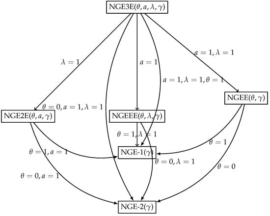
Figure 1. Relationship among submodels of the NGE3ED.

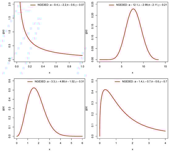
Figure 2. Pdf plots of NGE3ED.

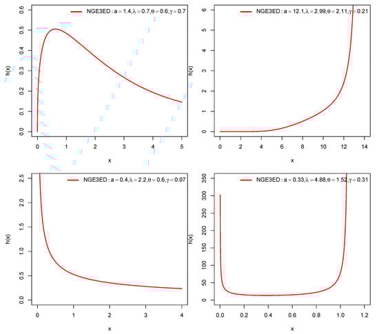
Figure 3. FRF plots of NGE3ED.

4.2. Quantile Function and Simulation Study

If $X\sim$ NGE3ED ($\theta ,a,\lambda ,\gamma$) has cdf (45), $G_{NGE3E}(x;\theta ,a,\lambda ,\gamma )$, the QF of X is

$$x_p=-\frac{1}{\gamma }log\left\{1-{\left[1-\frac{{(1-p)}^{\frac{1}{\lambda }}}{\theta }\mathbf{W}\left(\frac{\theta }{{(1-p)}^{\frac{1}{\lambda }}}exp(-\frac{1}{{(1-p)}^{\frac{1}{\lambda }}}[1-\theta -{(1-p)}^{\frac{1}{\lambda }}])\right)\right]}^{\frac{1}{a}}\right\}.$$

(48)

where $p\in (0,1)$, and $\mathbf{W}(.)$ the LWF.

Here, we give a Monte Carlo simulation study (MCSS) to assess the performance and accuracy of MLEs of NGE3ED parameters. The simulation study was performed with generation observations from parameter scenarios (I) $a=4.10,\lambda =2.99,\theta =2.11,\gamma =0.21$, and (II): $a=3.30,\lambda =4.88,\theta =1.52,\gamma =0.31$.

The number of MCSS replications was N = 10,000 with sample sizes $n=$ 50, 300, 550, 800, 1050, 1300, 1550, 1800, 2050. We used the $\mathtt{optim}\left(\right)$ R-function for maximizing the LLF of a probabilistic model. We examined the performance of MLEs for model “NGE3E” (a specific case of family) by computing the (i) average estimates (AEs), (ii) mean square errors (MSEs), and (iii) absolute biases (ABs).

$$Bias\left(\widehat{\mathrm{\Theta }}\right)=\sum _{i=1}^{10,000}\frac{{\widehat{\mathrm{\Theta }}}_i}{10,000}-\mathrm{\Theta },$$

and

$$MSE\left(\widehat{\mathrm{\Theta }}\right)=\frac{1}{10,000}\sum _{i=1}^{10,000}{({\widehat{\mathrm{\Theta }}}_i-\mathrm{\Theta })}^2.$$

The numerical and graphical results of MCSS are presented in Table 1 and Figure 4, Figure 5 and Figure 6. According to expectations, under the theory of first-order asymptotics, the MSEs and ABs decreased when n increased for Scenarios I and II. In this manner, the MLEs of NGE3ED parameters performed well.

Table 1. Simulation results for NGE3ED.

Set I: $\mathit{a}=4.10,\mathit{\lambda }=2.99,\mathit{\theta }=2.11,\mathit{\gamma }=0.21$					Set II: $\mathit{a}=3.30,\mathit{\lambda }=4.88,\mathit{\theta }=1.52,\mathit{\gamma }=0.31$
n	Parameter	MLE	MSE	AB	MLE	MSE	AB
50	$\widehat{a}$	4.178052	0.713267	0.078052	3.566745	1.041872	0.266745
	$\widehat{\lambda }$	2.639318	2.241914	0.350682	3.607051	4.074313	1.272949
	$\widehat{\theta }$	2.996142	2.892954	0.886142	2.542916	4.662988	1.022916
	$\widehat{\gamma }$	0.222999	0.007290	0.012999	0.383463	0.042189	0.073464
300	$\widehat{a}$	4.322833	0.380854	0.222833	3.625264	0.460963	0.325264
	$\widehat{\lambda }$	2.709852	1.547025	0.280148	3.434403	4.584252	1.445597
	$\widehat{\theta }$	2.243113	0.918195	0.133113	1.703476	0.713168	0.183476
	$\widehat{\gamma }$	0.243876	0.006906	0.033876	0.432456	0.047154	0.122456
550	$\widehat{a}$	4.265227	0.273629	0.165227	3.526255	0.245441	0.226255
	$\widehat{\lambda }$	2.852406	1.260532	0.137594	3.694286	3.433749	1.185714
	$\widehat{\theta }$	2.194856	0.586033	0.084856	1.610212	0.311643	0.090212
	$\widehat{\gamma }$	0.233397	0.004786	0.023397	0.398196	0.026787	0.088196
800	$\widehat{a}$	4.238538	0.217878	0.138538	3.471447	0.156626	0.171447
	$\widehat{\lambda }$	2.892669	1.054043	0.097331	3.875455	2.720822	1.004546
	$\widehat{\theta }$	2.168020	0.431818	0.058020	1.581829	0.180927	0.061829
	$\widehat{\gamma }$	0.228880	0.003738	0.018880	0.378363	0.017620	0.068363
1050	$\widehat{a}$	4.211064	0.170239	0.111064	3.446462	0.113253	0.146462
	$\widehat{\lambda }$	2.919116	0.895349	0.070884	3.971339	2.321943	0.908661
	$\widehat{\theta }$	2.157062	0.334494	0.047062	1.558690	0.119622	0.038690
	$\widehat{\gamma }$	0.225160	0.002968	0.015160	0.368524	0.012958	0.058524
1300	$\widehat{a}$	4.197459	0.140223	0.097459	3.416337	0.084250	0.116337
	$\widehat{\lambda }$	2.926014	0.764960	0.063986	4.078104	1.970276	0.801896
	$\widehat{\theta }$	2.141350	0.257725	0.031350	1.564415	0.101034	0.044415
	$\widehat{\gamma }$	0.223226	0.002444	0.013226	0.358211	0.009942	0.048211
1550	$\widehat{a}$	4.172582	0.116356	0.072582	3.407995	0.071701	0.107995
	$\widehat{\lambda }$	2.938682	0.651132	0.051318	4.132392	1.763364	0.747608
	$\widehat{\theta }$	2.150551	0.227299	0.040551	1.553020	0.080565	0.033020
	$\widehat{\gamma }$	0.220265	0.002023	0.010265	0.354000	0.008316	0.044000
1800	$\widehat{a}$	4.174525	0.104986	0.074525	3.391980	0.056767	0.091980
	$\widehat{\lambda }$	2.938528	0.594311	0.051472	4.200579	1.543466	0.679421
	$\widehat{\theta }$	2.136263	0.198713	0.026263	1.547978	0.065708	0.027978
	$\widehat{\gamma }$	0.220122	0.001831	0.010122	0.348373	0.006657	0.038373
2050	$\widehat{a}$	4.164815	0.092521	0.064815	3.382171	0.049089	0.082171
	$\widehat{\lambda }$	2.940650	0.523406	0.049350	4.242065	1.409728	0.637934
	$\widehat{\theta }$	2.138791	0.175037	0.028791	1.550037	0.059096	0.030037
	$\widehat{\gamma }$	0.218764	0.001610	0.008764	0.344838	0.005818	0.034838

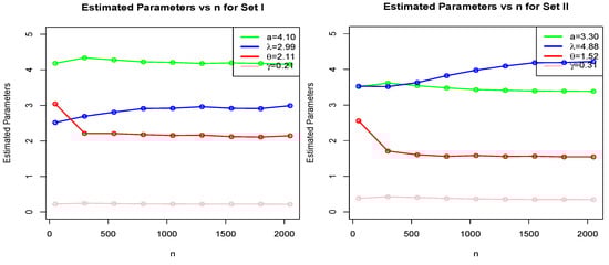
Figure 4. MLE plots of NGE3ED for Set I: $a=4.10,\lambda =2.99,\theta =2.11,\gamma =0.21$ and Set II: $a=3.30,\lambda =4.88,\theta =1.52,\gamma =0.31$.

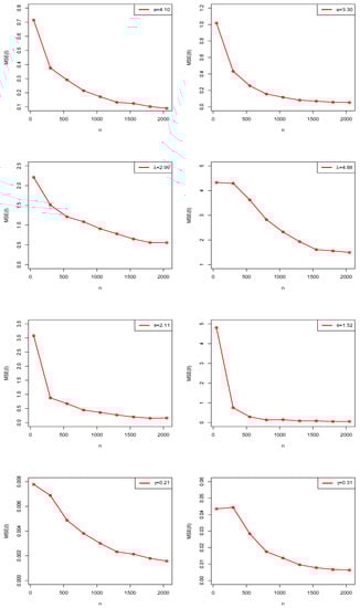
Figure 5. Estimated MSE plots of NGE3ED in MCSS.

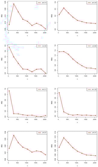
Figure 6. Estimated AB plots of NGE3ED in MCSS.

4.3. Estimation

Let a sample of size n be $x_1,x_2,\dots ,x_n$ from NGE3ED that has apdf in (46). The LLF for $\mathrm{\Theta }={(\theta ,a,\lambda ,\gamma )}^T$ is

$$\begin{array}{cc}\hfill L=L(\theta ,a,\lambda ,\gamma )=& nlog\left(a\gamma \lambda \right)-\gamma \sum _{i=1}^n{x}_i+(a-1)\sum _{i=1}^{n}log[1-exp(-\gamma x_i)]-\sum _{i=1}^{n}log[1-{\left(1-exp(-\gamma x_i)\right)}^a]+\hfill \\ \hfill & (\lambda -1)\sum _{i=1}^{n}log[1-\theta {\left(1-exp(-\gamma x_i)\right)}^a]-(\lambda +1)\sum _{i=1}^{n}log[1-log\{1-{\left(1-exp(-\gamma x_i)\right)}^a\}]+\hfill \\ \hfill & \sum _{i=1}^{n}log[\theta \{1-{\left(1-exp(-\gamma x_i)\right)}^a\}\{1-log[1-{\left(1-exp(-\gamma x_i)\right)}^a]\}+\{1-\theta {\left(1-exp(-\gamma x_i)\right)}^a\}].\hfill \end{array}$$

(49)

The LLF given in (49) can be maximized by utilizing the AdequacyModel package to obtain the MLEs of $\mathrm{\Theta }$. The components of the score function regarding $\theta ,a,\lambda$ and $\gamma$ are

$$\begin{array}{cc}\hfill \frac{\partial L}{\partial \theta }& =(1-\lambda )\sum _{i=1}^n\frac{{\left(1-exp(-\gamma x_i)\right)}^a}{1-\theta {\left(1-exp(-\gamma x_i)\right)}^a}+\hfill \\ \hfill & \sum _{i=1}^n\frac{\{1-{\left(1-exp(-\gamma x_i)\right)}^a\}\{1-log[1-{\left(1-exp(-\gamma x_i)\right)}^a]\}-{\left(1-exp(-\gamma x_i)\right)}^a}{\theta \{1-{\left(1-exp(-\gamma x_i)\right)}^a\}\{1-log[1-{\left(1-exp(-\gamma x_i)\right)}^a]\}+\{1-\theta {\left(1-exp(-\gamma x_i)\right)}^a\}},\hfill \end{array}$$

(50)

$$\begin{array}{cc}\hfill & \frac{\partial L}{\partial a}=\frac{n}{a}+\sum _{i=1}^{n}log[1-exp(-\gamma x_i)]+\sum _{i=1}^n\frac{{\left(1-exp(-\gamma x_i)\right)}^{a}log[1-exp(-\gamma x_i)]}{1-{\left(1-exp(-\gamma x_i)\right)}^a}-\theta (\lambda -1)\times \hfill \\ \hfill & \sum _{i=1}^n\frac{{\left(1-exp(-\gamma x_i)\right)}^{a}log[1-exp(-\gamma x_i)]}{1-\theta {\left(1-exp(-\gamma x_i)\right)}^a}-(\lambda +1)\sum _{i=1}^n\frac{{\left(1-exp(-\gamma x_i)\right)}^{a}log[1-exp(-\gamma x_i)]}{\{1-log[1-{\left(1-exp(-\gamma x_i)\right)}^a]\}\{1-{\left(1-exp(-\gamma x_i)\right)}^a\}}\hfill \\ \hfill & -\sum _{i=1}^n\frac{\theta {\left(1-exp(-\gamma x_i)\right)}^a\{1-log[1-{\left(1-exp(-\gamma x_i)\right)}^a]\}log[1-exp(-\gamma x_i)]}{\theta \{1-{\left(1-exp(-\gamma x_i)\right)}^a\}\{1-log[1-{\left(1-exp(-\gamma x_i)\right)}^a]\}+\{1-\theta {\left(1-exp(-\gamma x_i)\right)}^a\}},\hfill \end{array}$$

(51)

$$\begin{array}{c}\hfill \frac{\partial L}{\partial \lambda }=\frac{n}{\lambda }+\sum _{i=1}^{n}log[1-\theta {\left(1-exp(-\gamma x_i)\right)}^a]-\sum _{i=1}^{n}log[1-log[1-{\left(1-exp(-\gamma x_i)\right)}^a]],\end{array}$$

(52)

$$\begin{array}{cc}\hfill \frac{\partial L}{\partial \gamma }& =\frac{n}{\gamma }-\sum _{i=1}^n{x}_i+(a-1)\sum _{i=1}^n\frac{x_{i}exp(-\gamma x_i)}{1-exp(-\gamma x_i)}+a\sum _{i=1}^n\frac{x_i{\left(1-exp(-\gamma x_i)\right)}^{a-1}exp(-\gamma x_i)}{1-{\left(1-exp(-\gamma x_i)\right)}^a}+a(1-\lambda )\theta \times \hfill \\ \hfill & \sum _{i=1}^n\frac{{\left(1-exp(-\gamma x_i)\right)}^{a-1}{x}_{i}exp(-\gamma x_i)}{1-\theta {\left(1-exp(-\gamma x_i)\right)}^a}-a(1+\lambda )\sum _{i=1}^n\frac{x_{i}exp(-\gamma x_i){\left(1-exp(-\gamma x_i)\right)}^{a-1}}{\{1-log[1-{\left(1-exp(-\gamma x_i)\right)}^a]\}\{1-{\left(1-exp(-\gamma x_i)\right)}^a\}}\hfill \\ \hfill & -a\theta \sum _{i=1}^n\frac{x_i\{1-log[1-{\left(1-exp(-\gamma x_i)\right)}^a]\}{\left(1-exp(-\gamma x_i)\right)}^{a-1}exp(-\gamma x_i)}{\theta \{1-{\left(1-exp(-\gamma x_i)\right)}^a\}\{1-log[1-{\left(1-exp(-\gamma xi)\right)}^a]\}+\{1-\theta {\left(1-exp(-\gamma x_i)\right)}^a\}}.\hfill \end{array}$$

(53)

Setting

$$\frac{\partial L}{\partial \theta }=0,$$

(54)

$$\frac{\partial L}{\partial a}=0,$$

(55)

$$\frac{\partial L}{\partial \lambda }=0,$$

(56)

$$\frac{\partial L}{\partial \gamma }=0.$$

(57)

The MLEs $\widehat{\mathrm{\Theta }}$ of $\mathrm{\Theta }$ can be acquired by tackling NEs (54)–(57). These NEs cannot be tackled analytically, and to obtain the estimates numerically, a statistical package can be utilized. We can utilize iterative methods, for example, NRAs to obtain $\widehat{\mathrm{\Theta }}$ by utilizing a wide range of initial values.

4.4. Empirical Illustrations of the NGE3E Model

In this section, we match NGE3ED with some prominent generalized distributions. To illustrate the capability of NGE3ED, we analyze two real datasets. We compare the NGE3E model with the Weibull exponential (WE) (Oguntunde et al., 2015) [21], exponentiated WE (EWE) (Elgarhy et al., 2017) [22], exponentiated exponential Weibull (EEW) (Al Sulami, 2020) [23], beta exponential Fréchet (BEF) (Mead et al., 2017) [24], odd generalized exponential (OGE) Weibull (OGEW), OGE Fréchet (OGEFr) (Tahir et al., 2015) [25], exponentiated Kumaraswamy exponential (EKE) (Rodrigues and Silva, 2015) [26], Kumaraswamy weibull (KwW) (Cordeiro et al. 2010) [27], and Weibull Lomax (WL) (Tahir et al., 2014) [28] models through real-life datasets that are depicted below.

4.4.1. Dataset 1: Guinea Pig (GP) Data

From Bjerkedal (1960) [29], the survival time in days was taken from the dataset, consisting of 72 GPs infected with virulent tubercle bacilli. The observations are below:

	0.10	0.33	0.44	0.56	0.59	0.72	0.74	0.77	0.92	0.93
0.96	1.0	1.0	1.02	1.05	1.07	7.0	0.08	1.08	1.08	1.09
1.12	1.13	1.15	1.16	1.20	1.21	1.22	1.22	1.24	1.30	1.34
1.36	1.39	1.44	1.46	1.53	1.59	1.60	1.63	1.63	1.68	1.71
1.72	1.76	1.83	1.95	1.96	1.97	2.02	2.13	2.15	2.16	2.22
2.30	2.31	2.40	2.45	2.51	2.53	2.54	2.54	2.78	2.93	3.27
3.42	3.47	3.61	4.02	4.32	4.58	5.55

4.4.2. Dataset 2: Bladder Cancer (BC) Data

As reported by Ademola (2021) [30], a random sample, in months, of the remission times of 128 BC patients. The observations are as follows:

	0.08	2.09	22.69	12.63	3.48	4.87	8.65	6.93	6.94	8.66
3.36	2.07	13.11	23.63	21.73	12.07	0.20	2.23	6.76	3.36	3.52
4.98	2.02	20.28	6.97	9.02	12.03	8.53	13.29	0.40	6.54	4.51
2.26	3.57	3.31	2.02	5.06	7.09	9.22	12.02	13.80	8.37	25.74
6.25	0.50	4.50	2.46	3.25	3.46	1.76	5.09	19.13	7.26	11.98
9.47	8.26	14.24	5.85	25.82	4.40	0.51	1.46	2.54	18.10	3.70
11.79	5.17	7.93	7.28	5.71	9.74	4.34	14.76	3.02	26.31	1.40
0.81	4.33	17.36	2.83	11.64	1.26	7.87	46.12	5.62	17.12	2.87
7.63	1.35	79.05	5.41	17.14	4.26	11.25	2.75	7.66	1.19	5.49
43.01	10.66	16.62	7.59	5.34	4.18	10.75	7.62	2.69	5.41	0.90
4.23	34.26	2.69	14.83	1.05	10.34	36.66	7.39	15.96	5.32	3.88
2.64	32.15	14.77	10.06	7.32	5.32	3.82	2.62

The descriptive statistics (DSs) for the GP and BC datasets are presented in Table 2, and their box plots are shown in Figure 7a and Figure 8a, which demonstrate that distribution was skewed to the right. TTT plot of GP data displayed in Figure 7b reveal that the FRF was concave, suggesting an increasing failure rate shape, while the TTT plot of BC data in Figure 8b moved from concave to convex, giving an indication of UDBT-shaped failure rate. Accordingly, the NGE3E model could be suitable for fitting these datasets.

Table 2. DSs for Datasets 1 and 2.

Dataset	Min.	${\mathit{Q}}_1$	Median	${\mathit{Q}}_3$	Max.	Mean	Variance	Skewness	Kurtosis
1	0.080	1.080	1.560	2.303	7.000	1.837	1.478	1.755	4.152
2	0.080	3.348	6.395	11.838	79.050	9.366	110.425	3.287	15.483

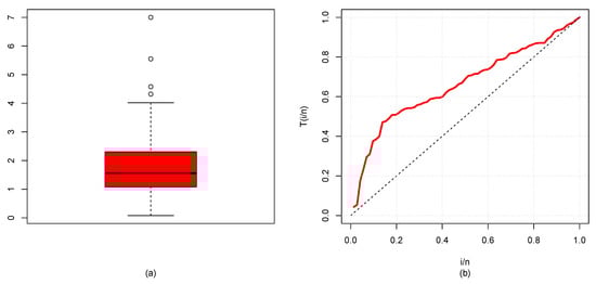
Figure 7. (a) Box plot and (b) TTT plot for GP data.

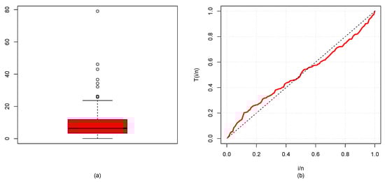
Figure 8. (a) Box plot (b) and TTT plot for BC data.

The pdfs of CMs are as follows:

• The EWE distribution

  $$g(x;a,\alpha ,\beta ,\lambda )=a\alpha \beta \lambda {\left(exp\left(\lambda x\right)-1\right)}^{\beta -1}{e}^{-\left\{\alpha {\left(exp\left(\lambda x\right)-1\right)}^{\beta }-\lambda x\right\}}{\left[1-e^{-\alpha {\left(exp\left(\lambda x\right)-1\right)}^{\beta }}\right]}^{a-1};x>0,a,\alpha ,\beta ,\lambda >0.$$
• WE distribution:

  $$g(x;\lambda ,\beta ,\alpha )=\lambda \beta \alpha {\left(1-exp(-\lambda x)\right)}^{\beta -1}exp(-\alpha {(exp\left(\lambda x\right)-1)}^{\beta }+\lambda \beta x);x>0,\lambda ,\beta ,\alpha >0.$$
• EEW distribution:

  $$g(x;\lambda ,\alpha ,\gamma ,\beta )=\lambda \alpha \gamma {\beta }^{-\gamma }{x}^{\gamma -1}exp(-\lambda {\beta }^{-\gamma }{x}^{\gamma }){\left[1-exp(-\lambda {\beta }^{-\gamma }{x}^{\gamma })\right]}^{\alpha -1};x>0,\lambda ,\alpha ,\gamma ,\beta >0.$$
• BEF distribution:

  $$\begin{array}{cc}\hfill g(x;\alpha ,\beta ,\lambda ,\gamma ,\theta )=& \frac{\gamma \lambda {\theta }^{\gamma }}{B(\alpha ,\beta )}{x}^{-(1+\gamma )}exp(-{\theta }^{\gamma }{x}^{-\gamma }){\left[1-exp(-{\theta }^{\gamma }{x}^{-\gamma })\right]}^{\lambda \beta -1}{\left[1-{\left\{1-exp(-{\theta }^{\gamma }{x}^{-\gamma })\right\}}^{\lambda }\right]}^{\alpha -1};\hfill \\ \hfill & x>0,\theta ,\gamma ,\lambda ,\beta ,\alpha >0.\hfill \end{array}$$
• OGEW distribution:

  $$g(x;\lambda ,\alpha ,\theta ,\beta )=\alpha \lambda \beta \theta x^{\beta -1}exp\left(\lambda -\lambda exp\left(\theta x^{\beta }\right)\right)exp\left(\theta x^{\beta }\right){\left[1-exp\left(\lambda -\lambda exp\left(\theta x^{\beta }\right)\right)\right]}^{\alpha -1};x>0,\alpha ,\beta ,\theta ,\lambda >0.$$
• OGEFr distribution:

  $$g(x;\theta ,\alpha ,\beta ,\lambda )=\lambda \alpha \beta {\theta }^{\beta }\frac{x^{-(\beta +1)}{e}^{-{\left(\frac{\theta }{x}\right)}^{\beta }}}{{\left(1-e^{-{\left(\frac{\theta }{x}\right)}^{\beta }}\right)}^2}exp\left(-\lambda \frac{e^{-{\left(\frac{\theta }{x}\right)}^{\beta }}}{1-e^{-{\left(\frac{\theta }{x}\right)}^{\beta }}}\right){\left[1-exp\left(-\lambda \frac{e^{-{\left(\frac{\theta }{x}\right)}^{\beta }}}{1-e^{-{\left(\frac{\theta }{x}\right)}^{\beta }}}\right)\right]}^{\alpha -1};x>0,\theta ,\alpha ,\beta ,\lambda >0.$$
• EKE distribution:

  $$g(x;\beta ,\lambda ,\theta ,\alpha )=\theta \lambda \beta \alpha {\left(1-e^{-\alpha x}\right)}^{\beta -1}{e}^{-\alpha x}{\left[1-{\left(1-e^{-\alpha x}\right)}^{\beta }\right]}^{\lambda -1}{\left[1-{\left(1-{(1-e^{-\alpha x})}^{\beta }\right)}^{\lambda }\right]}^{\theta -1};x>0,\lambda ,\beta ,\theta ,\alpha >0.$$
• KwW distribution:

  $$g(x;\gamma ,a,\alpha ,\beta )=\gamma a\alpha \beta x^{a-1}{e}^{-\gamma x^a}{\left(1-e^{-\gamma x^a}\right)}^{\alpha -1}{\left[1-{\left(1-e^{-\gamma x^a}\right)}^{\alpha }\right]}^{\beta -1};x>0,\gamma ,a,\alpha ,\beta >0.$$
• WL distribution:

  $$g(x;a,\beta ,\gamma ,\alpha )=a\beta \gamma \alpha {\left(1+\gamma x\right)}^{\alpha (\beta -1)}{\left[1-{\left(1+\gamma x\right)}^{-\alpha }\right]}^{\beta -1}exp\left\{-a{\left[{\left(1+\gamma x\right)}^{\alpha }-1\right]}^{\beta }\right\};x>0,a,\beta ,\gamma ,\alpha >0.$$

During the comparative analysis of the models, the $\mathtt{AdequacyModel}$ package of $\mathtt{R}$ was utilized to compute the application results. We adopted well-known goodness-of-fit measures (GFMs) such as $-\widehat{L}$ where $\widehat{L}$, is the maximized LLF, the Akaike information criterion (IC) (AIC), consistent AIC (CAIC), Bayesian IC (BIC), Cramer–von Mises (CM), Anderson–Darling (AD), and Kolmogorov–Smirnov (KS) statistics. In general, the model is the best fit with lower GFM values and a high p-value of the KS statistic.

MLEs with standard errors (SEs) for NGE3ED and CMs (EWE, WE, EEW, BEF, OGEW, OGEFr, EKE, KwW and WL) fitted to the guinea-pig and bladder-cancer datasets are listed in Table 3 and Table 4. The values of GFMs in Table 5 and Table 6 indicate that the NGE3E model gave small values of -L, AIC, CAIC, BIC, KS, CM, and AD, and a higher corresponding p-value. Hence, it showed a relatively better data fit than that of the CMs. Further, plots in Figure 9 and Figure 10 also support this conclusion.

Table 3. MLEs with SE (in parentheses) of CMs for guinea-pig data.

Dist.	$\widehat{\mathit{a}}$	$\widehat{\mathit{\lambda }}$	$\widehat{\mathit{\theta }}$	$\widehat{\mathit{\gamma }}$	$\widehat{\mathit{\alpha }}$	$\widehat{\mathit{\beta }}$
NGE3E	2.32272	5.56385	0.10187	0.31452	–	–
	(0.49245)	(7.00899)	(1.27805)	(0.18822)
EWE	2.29855	0.04199	–	–	21.89576	1.04688
	(1.21005)	(0.02975)			(19.11364)	(0.25627)
WE	–	0.03282	–	–	59.89789	1.54046
		(0.04996)			(162.26158)	(0.16146)
EEW	–	1.00906	–	1.15666	2.03844	1.33014
		(31.52095)		(0.27759)	(0.99803)	(35.93074)
BEF	–	0.65072	91.12759	0.40903	13.59632	5.60806
		(0.36349)	(41.07691)	(0.06542)	(52.52073)	(21.90342)
OGEW	–	21.13824	0.03953	–	2.42230	1.02483
		(38.08836)	(0.08007)		(1.41950)	(0.32531)
OGEFr	–	43.95769	45.57000	–	0.68169	0.44654
		(31.45097)	(32.38208)		(0.35684)	(0.08105)
EKE	–	16.65656	1.76429	–	0.08030	1.29005
		(65.36980)	(1.20989)		(0.28969)	(0.58900)
KwW	0.86432	–	–	0.53177	2.73100	3.21403
	(0.82088)			(0.46183)	(3.05683)	(9.65113)
WL	21.27763	–	–	0.70534	0.25353	2.19835
	(55.95618)			(0.84875)	(0.22020)	(0.54623)

Table 4. MLEs with SE (in parentheses) of CMs for bladder-cancer data.

Dist.	$\widehat{\mathit{a}}$	$\widehat{\mathit{\lambda }}$	$\widehat{\mathit{\theta }}$	$\widehat{\mathit{\gamma }}$	$\widehat{\mathit{\alpha }}$	$\widehat{\mathit{\beta }}$
NGE3E	1.46988	3.17280	0.04142	0.06681	–	–
	(0.22276)	(1.65586)	(0.76421)	(0.04233)
EWE	4.03707	0.01171	–	–	7.07212	0.52346
	(2.10918)	(0.00599)			(2.37210)	(0.11822)
WE	–	0.00691	–	–	13.77130	0.98836
		(0.00218)			(5.32372)	(0.06271)
EEW	–	0.75644	–	0.65442	2.79598	2.18408
		(41.90063)		(0.13484)	(1.26511)	(184.93870)
BEF	–	154.72736	92.01702	0.05378	153.63292	1.85484
		(256.89845)	(426.07475)	(0.03714)	(249.12744)	(2.52944)
OGEW	–	12.71015	0.04898	–	3.74616	0.53393
		(16.73725)	(0.07842)		(1.99784)	(0.15390)
OGEFr	–	0.03261	0.02360	–	2.53262	0.67782
		(0.03068)	(0.02448)		(1.01072)	(0.12675)
EKE	–	5.10315	3.89071	–	0.01387	0.48930
		(3.05943)	(3.16005)		(0.00977)	(0.23850)
KwW	0.46255	–	–	0.49332	4.08136	2.87041
	(0.39433)			(0.42793)	(4.52386)	(6.00747)
WL	14.27567	–	–	0.17142	0.17497	1.52178
	(26.47401)			(0.16655)	(0.15495)	(0.28860)

Table 5. GFMs of CMs for guinea-pig data.

Dist.	-L	AIC	CAIC	BIC	KS	p-Value	CM	AD
NGE3E	102.134	212.267	212.864	221.374	0.095	0.54	0.08360	0.57473
EWE	102.976	213.952	214.548	223.058	0.101	0.4569	0.11519	0.75801
WE	104.486	214.972	215.325	221.802	0.119	0.2632	0.17274	1.04466
EEW	102.810	213.620	214.217	222.726	0.101	0.4499	0.11008	0.72722
BEF	105.026	220.052	220.962	231.436	0.521	0.0000	0.12084	0.76687
OGEW	102.979	213.959	214.556	223.065	0.102	0.4421	0.11361	0.75265
OGEFr	105.679	219.353	219.950	228.460	0.131	0.1674	0.15307	1.07003
EKE	102.764	213.528	214.125	222.635	0.100	0.4704	0.11084	0.72641
KwW	102.710	213.420	214.017	222.526	0.101	0.4559	0.10771	0.71078
WL	102.781	213.562	214.159	222.668	0.105	0.4045	0.11242	0.73235

Table 6. GFMs of CMs for bladder-cancer data.

Dist.	-L	AIC	CAIC	BIC	KS	p-Value	CM	AD
NGE3E	409.823	827.645	827.971	839.053	0.037	0.9954	0.02147	0.14416
EWE	411.320	830.641	830.966	842.049	0.048	0.9244	0.05658	0.37454
WE	415.905	837.811	838.004	846.367	0.080	0.3840	0.16541	0.98962
EEW	410.680	829.360	829.685	840.768	0.045	0.9576	0.04367	0.28848
BEF	415.946	841.892	842.384	856.152	0.987	0.0000	0.20020	1.48189
OGEW	410.922	829.844	830.169	841.252	0.047	0.9427	0.04845	0.32110
OGEFr	410.838	829.676	830.001	841.084	0.044	0.9613	0.04767	0.31411
EKE	411.000	830.000	830.325	841.408	0.046	0.9459	0.05222	0.33891
KwW	410.569	829.138	829.464	840.546	0.045	0.9600	0.04145	0.27310
WL	410.165	828.329	828.655	839.737	0.043	0.9721	0.03296	0.21647

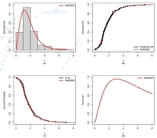
Figure 9. Estimated (a) pdf, (b) cdf, (c) Kaplan–Meier (K-M), and (d) hazard rate for guinea-pig data.

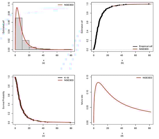
Figure 10. Estimated (a) pdf, (b) cdf, (c) Kaplan–Meier (K-M), (d) hazard rate for bladder-cancer data.

5. Conclusions

In this paper, the NGE3GF of distributions was characterized and examined. Various properties of this family were obtained, and special model of NGE3-Exponential (NGE3E) distribution was studied. Using popular GFM testing statistics, we compared NGE3ED with well-known GMs. NGE3ED provided better estimates with minimal GFMs and a high p value. On the basis of graphical and numerical analysis, the NGE3E distribution outclassed that of well-established CMs. We hope that NGE3GF will be able to attract researchers.

As future work, this study can be extended through a Bayesian technique to estimate the parameters of the different models derived from this proposed family. Moreover, other datasets in different areas can be used to check the flexibility of the derived models. This work can also be extended for bivariate Exponential Extended Exponentiated G-family of Distributions.

References

- Lemonte, A.J. A new exponential-type distribution with constant, decreasing, increasing, upside-down bathtub and bathtub-shaped failure rate function. Comput. Stat. Data Anal. 2013, 62, 149–170. [Google Scholar] [CrossRef]
- Adamidis, K.; Loukas, S. A lifetime distribution with decreasing failure rate. Stat. Probab. Lett. 1998, 39, 35–42. [Google Scholar] [CrossRef]
- Gupta, R.D.; Kundu, D. Exponentiated exponential family: An alternative to gamma and Weibull distribution. Biom. J. 2001, 43, 117–130. [Google Scholar] [CrossRef]
- Gupta, R.D.; Kundu, D. Generalized exponential distribution. Aust. N. Z. J. Stat. 1999, 41, 173–188. [Google Scholar] [CrossRef]
- Gupta, R.D.; Kundu, D. Generalized exponential distribution: Existing results and some recent developments. J. Stat. Plan. Inference 2007, 137, 3537–3547. [Google Scholar] [CrossRef]
- Balakrishnan, K. Exponential Distribution: Theory, Methods and Applications; CRC Press: Boca Raton, FL, USA, 2019. [Google Scholar]
- Johnson, N.L.; Kotz, S.; Balakrishnan, N. Related distributions and some generalizations. In Exponential Distribution: Theory, Methods and Applications; Balakrsihnan, K., Baus, A.P., Eds.; CRC Press: Boca Raton, FL, USA, 2019; pp. 297–306. [Google Scholar]
- Hussain, S.; Rashid, M.S.; Ul Hassan, M.; Ahmed, R. The Generalized Alpha Exponent Power Family of Distributions: Properties and Applications. Mathematics 2022, 10, 1421. [Google Scholar] [CrossRef]
- Martinez-Florez, G.; Bolfarine, H.; Gómez, H.W. A Unification of Families of Birnbaum-Saunders Distributions with Applications. Revstat-Stat. J. 2020, 18, 637–660. [Google Scholar] [CrossRef]
- Alzaatreh, A.; Lee, C.; Famoye, F. A new method for generating families of continuous distributions. Metron 2013, 71, 63–79. [Google Scholar] [CrossRef]
- Flajonet, P.; Odlyzko, A. Singularity analysis of generating function. SIAM J. Discr. Math. 1990, 3, 216–240. [Google Scholar] [CrossRef]
- Flajonet, P.; Sedgewich, R. Analytic Combinatorics; Cambridge University: Cambridge, MA, USA, 2009; ISBN 978-0-521-89806-5. [Google Scholar]
- Nielson, N. Handbuch der Theorie der Gamma Funktion; Chelsea Publishing Co.: New York, NY, USA, 1906. [Google Scholar]
- Ward, M. The representation of Stirling’s numbers and Stirling’s polynomials as sums of factorials. Am. J. Math. 1934, 56, 87–95. [Google Scholar] [CrossRef]
- Maple. Maplesoft, a Division of Waterloo Maple Incorporated, Ontario. 2016. Available online: https://www.maplesoft.com (accessed on 7 August 2022).
- Moors, J.J.A. A quantile alternative for kurtosis. Statistician 1998, 37, 25–32. [Google Scholar] [CrossRef]
- Kenney, J.; Keeping, E. Mathematics of Statistics, 3rd ed.; D. Van Nostrand: Princeton, NJ, USA, 1962; Volume 1. [Google Scholar]
- Smith, J.L.; Paul, D.; Paul, R. No place for a women: Evidence for gender bias in evaluations of presidential candidates. Basic Appl. Soc. Psych. 2007, 29, 225–233. [Google Scholar] [CrossRef]
- Renyi, A. On measures of entropy and information. Hung Acad. Sci. 1961, 1, 547–561. [Google Scholar]
- R Development Core Team. R: A Language and Environment for Statistical Computing; Foundation for Statistical Computing: Vienna, Austria, 2009. [Google Scholar]
- Oguntunde, P.E.; Balogon, O.S.; Okagbue, H.I.; Bishop, S.A. The Weibull-Exponential Distribution: Its Properties and Applications. J. Appl. Sci. 2015, 15, 1305–1311. [Google Scholar] [CrossRef]
- Elgarhy, M.; Shakil, M.; Golam Kibria, B.M. Exponentiated Weibull-Exponential Distribution with Applications. AAM Intern. J. 2017, 12, 710–725. [Google Scholar]
- Al Sulami, D. Exponentiated Exponential Weibull Distribution: Mathematical Properties and Application. Am. J. Appl. Sci. 2020, 17, 188–195. [Google Scholar] [CrossRef]
- Mead, M.E.; Afity, A.Z.; Hamedani, G.G.; Ghosh, I. The Beta Exponential Frechet Distribution with Applications. Austrian J. Stat. 2017, 46, 41–63. [Google Scholar] [CrossRef]
- Tahir, M.H.; Cordeiro, G.M.; Alizadeh, M.; Mansoor, M.; Zubair, M.; Hamedani, G.G. The odd generalized exponential family of distributions with applications. J. Stat. Distrib. Appl. 2015, 2, 1–28. [Google Scholar] [CrossRef]
- Rodrigues, J.A.; Silva, A.P.C.M. The Exponentiated Kumaraswamy Exponential Distribution. Br. J. Appl. Sci. Technol. 2015, 10, 1–12. [Google Scholar] [CrossRef]
- Cordeiro, G.M.; Ortega, E.M.M.; Nadarajah, S. The Kumaraswamy Weibull distribution with application to failure data. J. Frankl. Inst. 2010, 347, 1399–1429. [Google Scholar] [CrossRef]
- Tahir, M.H.; Cordeiro, G.M.; Mansoor, M.; Zubair, M. The Weibull-Lomax distribution: Properties and Applications. Hacet. J. Math. Stat. 2014, 44, 455–474. [Google Scholar] [CrossRef]
- Bjerkedal, T. Acquisition of resistance in Guinea Pies infected with different doses of Virulent Tubercle Bacilli. Am. J. Hyg. 1960, 72, 130–148. [Google Scholar]
- Ademola, A.A. Transmuted Sushila Distribution and its Application to Lifetime Data. J. Math. Anal. Model. 2021, 1, 1–14. [Google Scholar]
Publisher’s Note: MDPI stays neutral with regard to jurisdictional claims in published maps and institutional affiliations. |
© 2022 by the authors. Licensee MDPI, Basel, Switzerland. This article is an open access article distributed under the terms and conditions of the Creative Commons Attribution (CC BY) license (https://creativecommons.org/licenses/by/4.0/).