Abstract
This paper presents a control method for the problem of trajectory jitter and poor tracking performance of the end of a three-joint rigid manipulator. The control is based on a high-order particle swarm optimization algorithm with an improved sliding mode control neural network. Although the sliding mode variable structure control has a certain degree of robustness, because of its own switching characteristics, chattering can occur in the later stage of the trajectory tracking of the manipulator end. Hence, on the basis of the high-order sliding mode control, the homogeneous continuous control law and super-twisting adaptive algorithm were added to further improve the robustness of the system. The radial basis function neural network was used to compensate the errors in the modeling process, and an adaptive law was designed to update the weights of the middle layer of the neural network. Furthermore, an improved particle swarm optimization algorithm was established and applied to optimize the parameters of the neural network, which improved the trajectory tracking of the manipulator end. Finally, MATLAB simulation results indicated the validity and superiority of the proposed control method compared with other sliding mode control algorithms.
Keywords:
neural network; particle swarm optimization algorithm; sliding mode control; super-twisting adaptive algorithm; manipulators control MSC:
93d20; 68t073
1. Introduction
With the current development of technology, the application of robots has reached an unprecedented range, including aerospace, medical treatment, and welding. Robot application can not only reduce the labor intensity of workers but also improve the production efficiency. In addition, robots can be applied to tasks that need to be processed in inaccessible areas for humans. Therefore, manipulators play a crucial role in modern industry. Manipulators are based on the functions of human hands and arms and can be used for grasping, moving, and other complex operations similar to those carried out by human arms. Originally, a manipulator is operated by sequence control. With the optimization and development of computer intelligence, the control methods of manipulators as well as their application fields have diversified. This increment of robots also comes with a tremendous challenge, since each robot has a different structure and therefore each one requires a different algorithm to achieve its tasks [1]. The process of robot research mainly involves two aspects: trajectory planning and controller design. Complete trajectory planning includes path planning, inverse kinematics solution, and trajectory optimization [2]. For the trajectory tracking of robot manipulators, Carlos Lopez-Franco proposed a metaheuristic optimization approach to minimize the end-effector position and orientation in 3D [1]. Xiao et al. proposed an improved method of disconnection and reconnection to simplify the solution process of inverse kinematics. The solution of joint variables in the process of solving inverse kinematics is not affected by singularity [3]. Li et al. proposed a compensation method based on command posture to overcome the geometric parameter error compensation of the manipulator; this method cannot be effectively applied directly to the inverse kinematics of the nominal model of the manipulator, although the verification results show that this method takes less time than the Newton–Raphson algorithm [4]. In actual production, however, the control system of a manipulator can be interfered by a number of uncertainty factors, which decreases the positioning accuracy of the end effector of the manipulator. Hence, further research on the control method of a robot has practical significance [5]. An ideal control strategy considerably affects the output of a complex nonlinear system as well as the tracking of joints and ends. Researchers have been investigating perfect control strategies, such as adaptive control [6], sliding mode control (SMC) [7], and proportional–integral–derivative (PID) control [8], to achieve a faster and more efficient joint tracking. However, a single control strategy cannot meet all the requirements of trajectory tracking. Thus, multi-control strategies, for example, the sliding mode neural network control (SMNNC) [9], the fuzzy sliding mode neural network (FSMNNC) [10], the PID SMC [11], and the sliding mode neural network adaptive control (SMNNAC) [12], are combined so that they complement each other.
Owing to the chattering of SMC itself, the end trajectory cannot be tracked well. Therefore, research on the improvement of the chattering performance of SMC has gained attention. Kali et al. proposed a super-twisting algorithm (STA) with time delay estimation for realizing the high-precision trajectory tracking of robots in the presence of uncertainty and unexpected interference. The control law was designed on the basis of the STA to ensure robustness, finite time convergence, and chattering reduction [13]. For the robust tracking and modelling of the problems of uncertain time-delay systems, Pai proposed an NNSMC scheme with a dynamic output feedback radial basis function (RBF). This algorithm was based on dynamic output feedback SMC, the RBF neural network, and adaptive control. It solved the design of the sliding surface and the existence of the sliding mode. The validity of the scheme was also verified [14]. Zhang et al. designed an adaptive robust control strategy for the problems of low convergence speed and large positioning error of the conventional PID control in the trajectory tracking control of the manipulator. Compared with the conventional PID control, this strategy can more accurately control the trajectory of the manipulator end [15]. Scholars such as Liu et al. and Liao et al. used the RBF neural network to approximate the uncertainty in the modeling process of multi-joint manipulators and employed the adaptive control law to estimate the weights of the middle layer of the neural network. This reduced the tracking error of the end trajectory of the manipulator joint and improved the vibration phenomenon [16,17]. Liu et al. designed a self-tuning PSO fuzzy PID positioning controller to improve the robustness and accuracy of the controller. The simulation results showed that the transient response speed, tracking accuracy, and tracking system characteristics were significantly improved [18]. Liang et al. and Yang et al. designed an interference observer to observe and compensate the external uncertain interference for the multi-joint manipulator in the presence of external uncertain interference. Simulation verification demonstrated that the effect of the interference observer was significant, ensuring the control performance of the system [19,20].
The stable adaptive control for nonlinear systems using neural networks has received more and more attention in recent years. Sun et al. proposed a stable neural network-based adaptive controller design for integrating a neural network (NN) approach with an adaptive implementation of the variable structure control [21]. Sun proposed a stable adaptive controller of sampled-data nonlinear systems using neural networks by applying the approach to the stable neuro-adaptive control of rigid and flexible link robotic manipulators and obtained a set of stable sampled-data adaptive control approaches of robotic manipulators using neural networks [22].
When the RBF neural network is applied to approximate modeling errors and uncertain terms, the RBF often has complex surfaces with multiple poles owing to the loss function. The use of PSO to update the weights results in the model falling into the local optimal value easily. The following studies have improved the PSO algorithm. The well-established particle swarm optimization (PSO) algorithm was proposed to avoid the problem of early convergence that highly affects the original implementation of this algorithm [23]. The improved particle swarm optimization algorithm was derived from an evolutionary algorithm. The evolutionary computation algorithms are based on biological Darwinian evolution to design a solution and include ecology-based algorithms and bio-inspired algorithms. Ecology-based algorithms are based on the ecosystems to solve the problem. This group includes the biogeography-based optimization (BBO) and invasive weed colony optimization (IWO) algorithms. The bio-inspired algorithms include the particle swarm optimization algorithm (PSO), artificial bee colony algorithm (ABC), fish swarm algorithm (FSA), firefly algorithm (FA), bacterial foraging algorithm (BF), ant colony optimization algorithm (ACO) and others [24]. Evolutionary algorithms are also widely used. For example, Victor Parque et al. proposed using differential evolution (DE) to optimize the smooth curve fitting of mobile robot trajectories [25]. Alessandro Niccolaio et al. proposed the optimization of electric vehicles charging station deployment by means of evolutionary algorithms [23]. Liu et al. proposed an improved PSO algorithm to optimize the back propagation neural network (BPNN). The PSO algorithm used an improved adaptive acceleration factor and adaptive inertia weight to improve the initial weights and thresholds of the BPNN. The simulation results showed that the new algorithm can improve the convergence speed and prediction accuracy of the BPNN and reduce the prediction errors [26]. Wang et al. proposed a scheme in which the PSO algorithm was applied to optimize artificial neural networks (ANNs) and could effectively overcome the shortcomings of traditional neural networks with poor dynamic adaptability. That is, in traditional neural networks, it is usually necessary to perform iteration on the training samples for the process of weight convergence [27]. Zhang et al. proposed an improved PSO algorithm to optimize the PID neural network model. This new model was improved on the basis of the inertia weight and fitness function of the traditional PSO algorithm. The new model used the PSO algorithm to optimize the initial weight of the PID neural network, thereby shortening the study time for the optimal value of the particle swarm and reducing the chance of local minimum. The results indicated that this method has good self-learning ability, good optimization quality, high control accuracy, no overshoot, fast response, and short setting time [28]. For complex systems with high nonlinearity and strong coupling, Ye et al. used the decoupling control technology based on the PID neural network to eliminate the coupling between loops. However, the connection weights of the PID neural network can easily fall into local optimum. Hence, a hybrid PSO and differential evolution algorithm was proposed to optimize the connection weights of the PID neural network [29]. Yu et al. proposed a new evolutionary ANN algorithm. The improved PSO algorithm used methods including parameter automation strategies, speed resetting, crossover, and mutation, which significantly improved the performance of solution fine-tuning and the original PSO algorithm in global search. The improved PSO was employed to simultaneously evolve the structure and weight of the ANN through a specific individual representation and evolution scheme [30].
The aim of this paper was to design the controller for a three-joint manipulator; the modeling uncertainty in the system and external uncertainty interference were ignored. Even if the controller was designed by considering the various uncertainties in the system, its manipulator control performance was not sufficient, resulting in poor manipulator end trajectory tracking performance. In addition, there was obvious chattering in the later stage of the trajectory tracking of the manipulator end. To improve the manipulator’s operating performance and adaptability to the environment, Yun et al. proposed an automatic dynamic bit hybrid control method based on bit control and introduced an improved position controller based on the traditional fuzzy PID control strategy [31]. Therefore, in this study, a high-order SMC (HOSMC) based on an improved PSO neural network is proposed.
We used the Lagrange energy method to model the dynamics of the three-joint rigid manipulator. Subsequently, an HOSMC was designed for the dynamic model of the system, and a homogeneous continuous control law and super-twisting algorithm were added. In addition, an adaptive law was designed for the gain function of the super-twisting algorithm to enhance the robustness of the system. In view of factors such as the modeling uncertainty in the system, the RBF neural network was used to compensate and approximate the uncertainties. Moreover, the weights of the middle layer of the neural network were updated via the improved PSO algorithm. Finally, simulation experiments showed the superiority of the control method proposed in this paper.
The main contributions of this paper are as follows: (1) To address the problem of severe chattering of the system when approaching a sliding mode surface, the homogeneous continuous control term and the hyper spiral algorithm were added to the SMC, and the adaptive law was designed for the gain of the hyper spiral algorithm. (2) To deal with the model error and external uncertain interference in the process of system modeling, a neural network was used for approximation compensation. (3) To optimize the weights of the middle layer of the neural network, an improved PSO algorithm is used. (4) Tests were conducted on the improved PSO algorithm, and the results indicated that the proposed method has certain advantages in the tracking response speed and tracking error of a three-joint rigid manipulator.
The organizational structure of this paper is as follows. Section 2 presents details of related work and establishes a mathematical model of a three-joint manipulator. In Section 3, the SMC is designed, and in Section 4, high-order sliding mode control neural network adaptation is introduced. Section 5 presents the Proof of stability, and Section 6 presents the improved PSO algorithm to further optimize neural network parameters. In Section 7, simulation experiments are conducted on the algorithm. Finally, the conclusion is provided in Section 8.
2. Dynamic Modeling of a Three-Joint Rigid Manipulator
This paper considered a serial robot as an example, which satisfied the Pieper criterion of industrial robots. The first three joints of the manipulator were mainly responsible for the motion of the end position, and the latter three joints were responsible for the motion of the end posture. The dynamic parameter value of the former was larger, with obvious nonlinearity compared with that of the latter. To ensure that the simplified model maintained the generality of dynamics, the model was simplified with the first three degrees of freedom within the allowable error range, as shown in Figure 1.
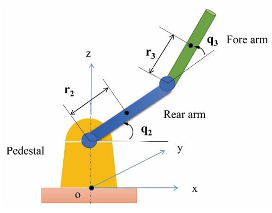
Figure 1.
Simplified model of the manipulator.
For = 1, 2, and 3, denotes the mass of the connecting rod , denotes the distance from joint to the center of gravity of the connecting rod , represents the length of the connecting rod , and represents the rotating angle of the connecting rod .
This model uses the Cartesian coordinate system. The centroid position of each joint is
The centroid velocity of each joint is
The total kinetic energy of the system is
The total potential energy of the system is
The Lagrange function of the system is
Substituting Equation (9), we obtain
The following can be obtained:
where
where
, , and are pseudo-inertial matrices.
The external uncertainty interference in the system is considered. Then, the dynamic equation of the system is
where
3. Sliding Mode Variable Structure Control
Let the state of the system be and . Then, the state equation of the system is
and , . Then, the control target is to track , where is the control input matrix, and represents uncertain external factors.
The error of the system is defined as
Then, the derivative of the error is
The sliding mode function is defined as
where is a positive integer greater than zero.
The derivation of the above equation is performed to obtain
The constant reaching law was used to reduce the chattering in the system and improve the robustness of the system. The constant reaching law is as follows:
where .
Then, the control law of the system is
The discrete switching characteristic of the traditional sliding mode variable structure control (SMC) leads to the oscillation of the system near the sliding mode surface, which leads to the chattering of the system at the later stage of trajectory tracking. Even with the addition of the constant velocity reaching law, the chattering of the system cannot be avoided; this leads to the degradation of the tracking performance.
4. High-Order Sliding Mode Neural Network Adaptive Control (HOSMC-NNA)
The sliding mode switch surface function is defined as
The derivation of the above equation is performed to obtain
Since the control signal of the manipulator does not appear in the first derivative of the sliding mode switch surface function, the derivative of the above formula is performed to obtain
If the finite time tracking of the system is considered, let and . Then,
The feedback control of the system is considered to obtain
Here, , where is a homogeneous continuous control term, with .
In this equation, , , , and . The continuous control law term makes the nominal system (that is, in the absence of external interference) converge to zero in a finite time.
In the presence of an external disturbance of the system, , the stability of the system cannot be guaranteed for a finite time when the auxiliary control item only considers the homogeneous continuous control law . Hence, the second-order sliding mode super spiral algorithm [32] is employed to achieve the robustness of the system.
where is a super-twisting function, and and are the super-twisting function control gains. The adaptive law can be designed as
where , , and are constants. In addition, should be ensured to be a positive definite matrix.
The uncertainty in the modeling process of the system can reduce the trajectory tracking performance of the system. Although the homogeneous continuous control term and the super-twisting adaptive algorithm are added to the control law, the control law cannot compensate the modeling uncertainty in the system.
In the expression , contains all the model uncertainty information. The goal is to use the RBF neural network to approximate .
The RBF is a Gaussian function, expressed as with = 1, 2… m, where x is the input of the RBF neural network, is the center value of the input data, and is the expansion constant or base width of the basis function. In
W is the weight in the middle layer of the RBF neural network, and is a small positive real number, representing the approximation error of the neural network to the nonlinear uncertainty function. In
is the approximation of the neural network to function , and is the ideal weight.
The above two equations are combined to obtain the following equation.
where .
The RBF neural network weight adaptive law is designed as
where γ is a positive constant greater than zero, , P is a symmetric positive definite matrix, 𝐵 = [0 1]𝑇, h is the neural network function.
This method uses a high-order sliding mode control, a homogeneous continuous control, and a super-spiral adaptive algorithm and thus can effectively reduce the chattering of the system. At the same time, the neural network adaptive control algorithm is used to compensate the system modeling errors. Thus, this method not only speeds up the trajectory tracking performance but also enhances the robustness of the system. The weights of the middle layer of the neural network are adjusted by the designed adaptive law. However, the method has a low convergence speed and i can easily fall into the local optimum.
5. Proof of Stability
A stable adaptive controller design for manipulators using neural networks has been proposed, and the stability analysis of an RBF neural network control scheme has been performed for a robot manipulator [33].
Define the matrix ; when and , is a Hurwitz matrix. Therefore, for any positive definite matrix , there must be a positive definite symmetric matrix that satisfies the Lyapunov equation:
Define the matrix , where and are taken as the upper bounds of and , respectively. Next, define the errors and ; then .
Define the Lyapunov function as
where is a continuous positive definite function and is radially unbounded. Therefore, it can be derived by the chain rule.
Assume ,
Consider
From the derivation of Equation (36), we obtain
From the derivation of Equation (35), we obtain
Given that
we have
We have
where
For , we obtain
Then,
If , then
Consequently,
The approximation error of the neural network model is defined as:
where is the optimal weight.
The overall Lyapunov function is considered as follows:
From the derivation of Equation (50), we get
By substituting the adaptive law (29) into Equation (51), we obtain
where is the model approximation error. The model approximation error is small enough so that .
According to the Lyapunov stability theory, the system is stable in a finite time.
6. Improved Particle Swarm Optimization Algorithm (IPSO)
In the basic PSO algorithm, each particle corresponds to a feasible solution of an optimization problem. The quality of the particles is determined by the fitness function set in advance.
In the traditional PSO algorithm, the convergence accuracy of the algorithm is low. Furthermore, in the later stage of the algorithm convergence, the reduction in particle swarm diversity causes the algorithm to fall into the local optimum, that is, the algorithm becomes “premature”. Moreover, particles are easily trapped in the poor search area and cannot easily escape. This can lead to search stagnation, resulting in a reduction in the algorithm convergence efficiency. To effectively avoid the above-mentioned problems, this paper proposes an improved PSO algorithm.
The particle-update formula of the traditional PSO algorithm includes three parts: the velocity value of the previous-generation particle, the learning part of a single particle, and the mutual learning part between particle swarms. The first part is controlled by the weighting factor , the second part is controlled by the acceleration factor , and the third part is controlled by the acceleration factor . In order to improve the global search ability of the PSO in the initial stage, the chaos theory was used to initialize the initial particle swarm. It is expressed as
where represents the initial value, which is a random number in the interval of (0,1), represents the logistic parameter, and . When is close to 4, the sequence generated by the logistic model has the characteristics of aperiodicity and non-convergence. Hence, a = 4 was adopted.
Therefore, the above formula became
The chaotic motion is traversed by various states in its chaotic attraction domain without losing the randomness requirement of particle swarm initialization. Therefore, the sequence generated by chaos has the characteristics of divergence and randomness such that it can improve the group search ability of the particle swarm.
In the PSO algorithm, the variance of the group fitness, that is, the entropy between particles, is used to evaluate the degree of convergence or dispersion of all particles in the swarm. The larger the value of , the larger can be the entropy value between the particles in a swarm, which means that the more dispersed the particles are, whereas, in the opposite situation, the more the particles converge. The formula for calculating the entropy between particles in a swarm is as follows:
where represents the fitness value of the i-th particle, and represents the mean value of the particle fitness values in the current particle swarm:
The improved formula of inertia weight is
where
here, is the current iteration number, and is total number of iterations. The improved acceleration constants are
where and are the initial values of and , respectively.
When , the diversity of the particles in the swarm population is poor, and the algorithm is more likely to fall into the local optimal solution. Therefore, the following formula is used to update the position of the particles, which lets the particles overcome the local optimal solution.
To verify the validity of the IPSO algorithm, in this paper, five standard test functions were randomly selected for function optimization. The basic mathematical properties of the selected five standard test functions are shown in Table 1, where U represents a single peak, M represents multiple peaks, N represents inseparable peaks, and S represents separable peaks. To ensure the validity of the data obtained in the experiment, 50 statistical experiments were performed for each standard test function. The optimal value, average optimal value (Mean), and standard deviation (Std) according to the statistical results were calculated. In addition, the performance of the IPSO algorithm was evaluated and compared with that of the traditional PSO algorithm. For both algorithms, the same parameters were set, with the number of populations being 50, and the number of iterations being 200. The experimental results are shown in Table 2.

Table 1.
Standard test functions.
Table 2.
Function optimization results.
For different types of functions, , , , , , with different dimensions, we compared the traditional particle swarm optimization algorithm with the improved particle swarm optimization algorithm. The functions and are unimodal functions and were mainly used to test the convergence speed and optimization accuracy of the algorithm degree. The functions , , and are multi-modal functions, which were mainly used to test the ability of the algorithm to jump out of the local optimum and avoid “premature” convergence. It can be seen from Table 1 and Table 2 that the improved particle swarm optimization algorithm could obtain the optimal value on both unimodal and multi-modal functions, but it was significantly better than the traditional particle swarm optimization algorithm in terms of accuracy of the convergence speed.
From the mean and standard deviation, it can be seen that the stability of the IPSO algorithm was better than that of the traditional PSO algorithm. Therefore, this paper used the IPSO algorithm to optimize the weights of the middle layer of the radial basis function neural network, so as to improve the approximation and compensation performance of the radial basis function neural network for the modeling uncertainty information in the manipulator system. In summary, the IPSO algorithm could achieve a relatively high convergence accuracy and was better than the traditional PSO algorithm. Figure 2 shows the flow chart of the particle swarm optimization neural network.
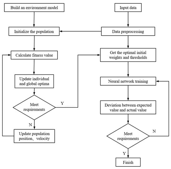
Figure 2.
Flow chart of the particle swarm optimization neural network.
As shown in Figure 2, the first step was to build an environment model. The second step of the proposed model was to initialize the population with a random method in which the preprocessing data were input. The third step consisted in calculating the fitness value for calculating the entropy between the particles in a swarm using Equation (56). The fourth step involved updating the individual and globally optimizing population position and velocity. These steps were repeated until the requirements were satisfied. We then performed the fifth step and obtained the optimal initial weights and threshold the number of iterations or the error rate. If this was not achieved, the calculated fitness value was rejected until the conditions were met. The sixth step consisted in performing the neural network training. The seventh step is allowed obtaining the deviation between the expected value and the actual value. These steps were repeated until the stop condition was satisfied. Figure 3 shows the proposed control strategy.
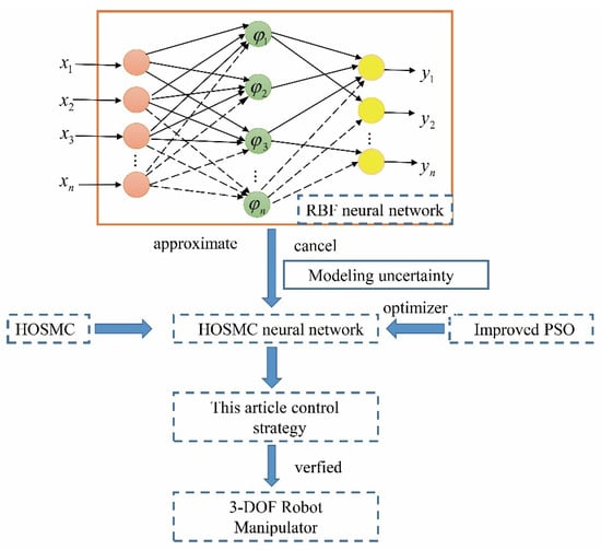
Figure 3.
Control strategy block diagram.
As shown in Figure 3, this study control strategy included the high-order sliding mode control (HOSMC), aiming at the uncertainty of system modeling. A neural network (NN) was adopted, and the improved particle swarm optimization algorithm (IPSO) was used to optimize the neural network. Finally, this method (HOSMC-NN-IPSO) was verified in a 3-DOF robot manipulator.
7. Simulation Analysis
A three-joint rigid manipulator was considered in the simulation analysis. The system parameters were as follows: , , , , , , , , , , and , where 1, 2, and 3, correspond to joints 1–3, respectively. In the design of the RBF neural network, the network structure was set to 2-7-1; the input of the neural network was ; the ideal position tracking curves in the system were obtained as , , and ; the initial state of the system was set to ; the external disturbance in the system was . In the IPSO algorithm, ; the number of populations was 50; the number of iterations was 200. The simulation was performed on MATLAB/Simulink, and the results are shown in Figure 4, Figure 5, Figure 6 and Figure 7.
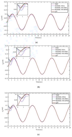
Figure 4.
Position tracking of the joints under the SMC, HOSMC−NNA, HOSMC−NN−PSO and HOSMC−NN−IPSO controllers. (a) Position tracking of the joint 1. (b) Position tracking of the joint 2. (c) Position tracking of the joint 3.
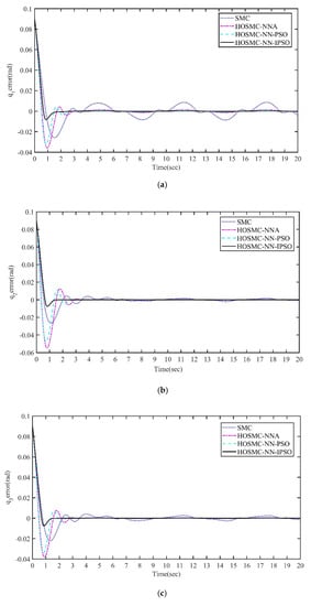
Figure 5.
Position tracking error of the joints under the SMC, HOSMC−NNA, HOSMC−NN−PSO and HOSMC−NN−IPSO controllers. (a) Position tracking error of the joint 1. (b) Position tracking error of the joint 2. (c) Position tracking error of the joint 3.
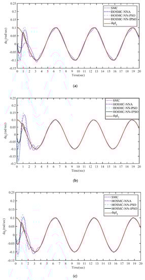
Figure 6.
Angular velocity tracking of joints under SMC, HOSMC−NNA, HOSMC−NN−PSO and HOSMC−NN−IPSO controllers. (a) Angular velocity tracking of joint 1. (b) Angular velocity tracking of joint 2. (c) Angular velocity tracking of joint 3.
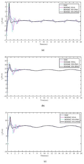
Figure 7.
Control input of the joints under the SMC, HOSMC−NNA, HOSMC−NN−PSO and HOSMC−NN−IPSO controllers. (a) Control input of the joint 1. (b) Control input of the joint 2. (c) Control input of the joint 3.
The figures show the curves of position tracking (Figure 4), tracking error (Figure 5), angular velocity tracking (Figure 6), and control input (Figure 7) of joints 1–3 under different controllers, namely, SMC, HOSMC−NNA, high−order sliding mode neural network control based on the PSO algorithm (HOSMC−NN−PSO), and high-order sliding mode neural network control based on the improved PSO algorithm (HOSMC−NN−IPSO).
For joint 1, as shown in Figure 4a, compared with other methods, HOSMC−NN−IPSO showed a faster and more effective position tracking performance. As shown in Figure 5a, HOSMC−NN−IPSO had the smallest tracking error of within a finite time and converged to zero faster. Figure 4a and Figure 5a show that HOSMC−NN−IPSO reduced the maximum overshoot.
Figure 4b shows that HOSMC−NN−PSO also completed position tracking within 2 s, while Figure 5b shows that its tracking error was significantly larger (by 0.45) than that of HOSMC−NN−IPSO. As shown in Figure 5a–c, especially in Figure 5a, the position tracking error of joints 1, 2, and 3 was significantly smaller with the HOSMC−NNA, HOSMC−NN−PSO, and HOSMC−NN−IPSO controllers than with the SMC, which illustrates the effect of the RBF neural network control in stability control.
Figure 6b shows that HOSMC−NN−PSO and HOSMC−NN−IPSO could complete the velocity tracking of . However, the chattering of HOSMC−NN−IPSO was significantly reduced compared with that of other methods.
Figure 4c shows the position tracking of HOSMC−NN−IPSO for joint 3. HOSMC−NN−IPSO not only converged to the tracking curve faster but also considerably eliminated the chattering in the later stage. Figure 6c also shows that HOSMC−NN−IPSO had obvious advantages over other methods in minimizing the chattering in the later stage.
Figure 7a–c show that the control input of the HOSMC−NN−IPSO method converged faster than that of other methods and tended to stabilize within 2 s; thus, the chattering caused by SMC was eliminated in the later stage.
8. Conclusions
In this paper, a high-order sliding mode control method based on an improved PSO neural network is proposed for three-joint rigid manipulators. Among the various controllers studied in this paper, HOSMC−NN−IPSO was the fastest in tracking the trajectory of the manipulator. Moreover, in the later stage of the tracking, its tracking error was the smallest and could converge to 0 faster compared with other controllers. The control input of each joint manipulator could be smoothed after 2 s with small chattering in the later stage. Therefore, the proposed HOSMC−NN−IPSO controller showed a good trajectory tracking performance. It appears that it cannot only track the ideal trajectory quickly but also guarantee the performance of the system in the later stage of trajectory tracking. Furthermore, the system is more robust than other controllers.
In this control method, the homogeneous continuous control law and super-twisting adaptive algorithm were included to further strengthen the robustness of SMC. In addition, for the modeling of uncertainty in the system, the RBF neural network was used to approximate and compensate the modeling uncertainty in the system. The weights of the middle layer of the neural network were updated by applying an IPSO algorithm. Finally, the MATLAB simulation results comparing different algorithms validated the proposed high-order sliding mode neural network adaptive control and high-order sliding mode neural network with IPSO control and confirmed their superiority over SMC.
Author Contributions
J.Z. is responsible for algorithm writing, testing, and thesis writing. Y.Y. and Z.L. are responsible for obtaining key data. W.L. and L.M. are participants of the study. W.M. is the project leader. All authors have read and agreed to the published version of the manuscript.
Funding
This study was financially supported by the National Key R&D Program of China for Robot Project (grant number 2018YFB1308700), the Shanxi Provincial Key Core Technologies and Common Technology Special Projects (grant number 2020XXX009), and the Science and Technology Project of the Shanxi Provincial Department of Transportation (grant number 2019-01-09).
Data Availability Statement
Data are contained within the article.
Conflicts of Interest
The authors declare no conflict of interest.
Nomenclature
| Rotation angle at manipulator joint | |
| System kinetic energy | |
| System’s potential | |
| Mass matrix | |
| Coriolis force and centrifugal force matrix | |
| Gravity matrix | |
| Control input matrix | |
| Uncertain external factors | |
| Sliding mode surface function | |
| Homogeneous continuous control term | |
| Super-twisting function | |
| Super-twisting l function control gain | |
| Super-twisting function control gain | |
| Output of the Gauss function. | |
| Weights of the intermediate layer | |
| Lyapunov stability function | |
| Position of any particle in the swarm | |
| Velocity of any particle in the swarm | |
| Best position experienced by the particles in the swarm | |
| Best position experienced by the swarm in the swarm | |
| Inertial weight | |
| Acceleration constant usually called the cognitive learning factor | |
| Acceleration constant usually called the social learning factor |
References
- Lopez-Franco, C.; Diaz, D.; Hernandez-Barragan, J.; Arana-Daniel, N.; Lopez-Franco, M. A Metaheuristic Optimization Approach for Trajectory Tracking of Robot Manipulators. Mathematics 2022, 10, 1051. [Google Scholar] [CrossRef]
- Zhang, X.; Xiao, F.; Tong, X.; Yun, J.; Liu, Y.; Sun, Y.; Tao, B.; Kong, J.; Xu, M.; Chen, B. Time Optimal Trajectory Planing Based on Improved Sparrow Search Algorithm. Front. Bioeng. Biotechnol. 2022, 10, 14. [Google Scholar] [CrossRef] [PubMed]
- Xiao, F.; Li, G.; Jiang, D.; Xie, Y.; Yun, J.; Liu, Y.; Li, H. An effective and unified method to derive the inverse kinematics formulas of general six-DOF manipulator with simple geometry. Mech. Mach. Theory 2021, 14, 104265. [Google Scholar] [CrossRef]
- Li, G.; Xiao, F.; Zhang, X.; Tao, B.; Jiang, G. An inverse kinematics method for robots after geometric parameters compensation. Mech. Mach. Theory 2022, 174, 104903. [Google Scholar] [CrossRef]
- Dong, J.; Chen, L. The nonlinear integral sliding mode of RBF neural network algorithm is used to control the motion trajectory error of the manipulator. Chin. J. Constr. Mach. 2018, 16, 106–110. [Google Scholar] [CrossRef]
- Khan, S.G.; Herrmann, G.; Pipe, T.; Melhuish, C.; Spiers, A. Safe adaptive compliance control of a humanoid robotic arm with anti-windup compensation and posture control. Int. J. Soc. Robot. 2010, 2, 305–319. [Google Scholar] [CrossRef]
- Rahmani, M.; Komijani, H.; Rahman, M.H. New sliding mode control of 2-DOF robot manipulator based on extended grey wolf optimizer. Int. J.Control. Autom. Syst. 2020, 18, 1572–1580. [Google Scholar] [CrossRef]
- Asl, R.M.; Pourabdollah, E.; Salmani, M. Optimal fractional order PID for a robotic manipulator using colliding bodies design. Soft Comput. 2018, 22, 4647–4659. [Google Scholar] [CrossRef]
- Li, Z.; Yin, Y.; Zhang, J.; Qi, C. Disturbance observer control of the multi-joint manipulator based on the backstepping sliding mode's neural network. J. Mach. Des. 2021, 38, 126–131. [Google Scholar] [CrossRef]
- Wang, T. Research on obstacle avoidance of wheeled mobile robot based on wavelet neural network and fuzzy sliding mode control. Chin. J. Constr. Mach. 2020, 18, 278–282. [Google Scholar] [CrossRef]
- Noordin, A.; Basri, M.A.M.; Mohamed, Z.; Lazim, I.M. Adaptive PID controller using sliding mode control approaches for quadrotor UAV attitude and position stabilization. Arab. J. Sci. Eng. 2021, 46, 963–981. [Google Scholar] [CrossRef]
- Zhang, J.; Li, Z.; Yin, Y.; Qi, C.; Wu, K. High-order sliding mode neural network adaptive control of multi-joint manipulator. Mech. Sci. Technol. Aerosp. Eng. 2021, 40, 710–715. [Google Scholar] [CrossRef]
- Kali, Y.; Saad, M.; Benjelloun, K.; Khairallah, C. Super-twisting algorithm with time delay estimation for uncertain robot manipulators. Nonlinear Dyn. 2018, 93, 557–569. [Google Scholar] [CrossRef]
- Pai, M.-C. Dynamic output feedback RBF neural network sliding mode control for robust tracking and model following. Nonlinear Dyn. 2015, 79, 1023–1033. [Google Scholar] [CrossRef]
- Zhang, C.; Zhang, Z. Application of adaptive robust control of the manipulator trajectory tracking. Modul. Mach. Tool Autom. Manuf. 2019, 86–89+93. [Google Scholar] [CrossRef]
- Liu, Y.; Chen, J. Research on trajectory error of mechanical arm based on radial basis function neural network control. Mach. Tool Hydraul. 2018, 46, 105–108. [Google Scholar]
- Liao, L.; Yang, Y. Adaptive radial basis function neural network bi-quadratic functional optimal control for manipulators. Control. Theory Appl. 2020, 37, 47–58. [Google Scholar]
- Liu, Y.; Jiang, D.; Yun, J.; Sun, Y.; Li, C.; Jiang, G.; Kong, J.; Tao, B.; Fang, Z. Self-Tuning Control of Manipulator Positioning Based on Fuzzy PID and PSO Algorithm. Front. Bioeng. Biotechnol. 2022, 9, 817723. [Google Scholar] [CrossRef]
- Liang, H.; Mi, G. An improved reaching law of sliding mode control for robotic manipulator based on disturbance observer. Meas. Control. Technol. 2019, 38, 140–144. [Google Scholar] [CrossRef]
- Yang, Y.; Wang, S. High-order sliding mode interference observer based on space flexible manipulator for trajectory tracking. Transducer Microsyst. Technol. 2019, 38, 114–117+128. [Google Scholar] [CrossRef]
- Sun, F.; Sun, Z. Stable Adaptive Controller Desigh for Manipulators Using Neural Networks. Control. Theory Appl. 1997, 14, 809–816. [Google Scholar]
- Sun, F. Stable Adaptive Control of Robot Manipulators Using Neural Networks. Ph.D. Thesis, Tsinghua University, Beijing, China, 1997. [Google Scholar]
- Niccolai, A.; Bettini, L.; Zich, R. Optimization of electric vehicles charging station deployment by means of evolutionary algorithms. Int. J. Intell. Syst. 2021, 36, 5359–5383. [Google Scholar] [CrossRef]
- Faculty of Sciences and Techniques of Sidi Bouzid, U.o.K., Tunisia; Dhahri, H. Biogeography-Based Optimization for Weight Optimization in Elman Neural Network Compared with Meta-Heuristics Methods. Brain Broad Res. Artif. Intell. Neurosci. 2020, 11, 82–103. [Google Scholar] [CrossRef]
- Parque, V.; Miyashita, T. Smooth Curve Fitting of Mobile Robot Trajectories Using Differential Evolution. IEEE Access 2020, 8, 82855–82866. [Google Scholar] [CrossRef]
- Liu, T.; Yin, S. An improved particle swarm optimization algorithm used for BP neural network and multimedia course-ware evaluation. Multimed. Tools Appl. 2017, 76, 11961–11974. [Google Scholar] [CrossRef]
- Wang, J.; Yang, H.; Hu, X.; Wang, X. An adaline neural network-based multi-user detector improved by particle swarm optimization in CDMA systems. Wirel. Pers. Commun. 2011, 59, 191–203. [Google Scholar] [CrossRef]
- Zhang, H.; Yuan, X. An improved particle swarm algorithm to optimize PID neural network for pressure control strategy of managed pressure drilling. Neural Comput. Appl. 2020, 32, 1581–1592. [Google Scholar] [CrossRef]
- Ye, H.-T.; Li, Z.-Q. PID neural network decoupling control based on hybrid particle swarm optimization and differential evolution. Int. J. Autom. Comput. 2020, 17, 867–872. [Google Scholar] [CrossRef]
- Yu, J.; Xi, L.; Wang, S. An improved particle swarm optimization for evolving feedforward artificial neural networks. Neural Process. Lett. 2007, 26, 217–231. [Google Scholar] [CrossRef]
- Yun, J.; Sun, Y.; Li, C.; Jiang, D.; Tao, B.; Li, G.; Liu, Y.; Chen, B.; Tong, X.; Xu, M. Self-adjusting force/bit blending control based on quantitative factor-scale factor fuzzy-PID bit control. Alex. Eng. J. 2022, 61, 4389–4397. [Google Scholar] [CrossRef]
- Rahmani, M.; Komijani, H.; Ghanbari, A.; Ettefagh, M.M. Optimal novel super-twisting PID sliding mode control of a MEMS gyroscope based on multi-objective bat algorithm. Microsyst. Technol. 2018, 24, 2835–2846. [Google Scholar] [CrossRef]
- Jung, S. Stability analysis of reference compensation technique for controlling robot manipulators by neural network. Int. J. Control. Autom. Syst. 2017, 15, 952–958. [Google Scholar] [CrossRef]
Publisher’s Note: MDPI stays neutral with regard to jurisdictional claims in published maps and institutional affiliations. |
© 2022 by the authors. Licensee MDPI, Basel, Switzerland. This article is an open access article distributed under the terms and conditions of the Creative Commons Attribution (CC BY) license (https://creativecommons.org/licenses/by/4.0/).