Article

Positive-Unlabeled Learning for Network Link Prediction

1
College of Computer, Hubei University of Education, Wuhan 430205, China
2
College of Computer Science and IT, Albaha University, Albaha 65515, Saudi Arabia
3
College of Informatics, Huazhong Agricultural University, Wuhan 430070, China
*
Author to whom correspondence should be addressed.
Mathematics 2022, 10(18), 3345; https://doi.org/10.3390/math10183345
Submission received: 22 August 2022 / Revised: 6 September 2022 / Accepted: 13 September 2022 / Published: 15 September 2022
(This article belongs to the Special Issue Class-Imbalance and Cost-Sensitive Learning)

Abstract

:
Link prediction is an important problem in network data mining, which is dedicated to predicting the potential relationship between nodes in the network. Normally, network link prediction based on supervised classification will be trained on a dataset consisting of a set of positive samples and a set of negative samples. However, well-labeled training datasets with positive and negative annotations are always inadequate in real-world scenarios, and the datasets contain a large number of unlabeled samples that may hinder the performance of the model. To address this problem, we propose a positive-unlabeled learning framework with network representation for network link prediction only using positive samples and unlabeled samples. We first learn representation vectors of nodes using a network representation method. Next, we concatenate representation vectors of node pairs and then feed them into different classifiers to predict whether the link exists or not. To alleviate data imbalance and enhance the prediction precision, we adopt three types of positive-unlabeled (PU) learning strategies to improve the prediction performance using traditional classifier estimation, bagging strategy and reliable negative sampling. We conduct experiments on three datasets to compare different PU learning methods and discuss their influence on the prediction results. The experimental results demonstrate that PU learning has a positive impact on predictive performances and the promotion effects vary with different network structures.

1. Introduction

The growing number of complex systems including social networks, biological information networks and paper citation networks can be represented as network structures, which has injected new vitality into the development of network data mining. Various network-based data mining problems are now being studied, such as heterogeneous network analysis [1,2,3], community discovery [4,5] and network visualization [6]. Link prediction is one of the most interesting network-related problems whose purpose is to infer whether there are new relationships or interactions between nodes based on the attributes of nodes in the network and the observed links [7,8]. Plenty of methods and technologies have been proposed to solve this problem using the hidden information of the network topology to predict potential links and estimate the evolution of the network [9].
Traditional link prediction in the network can be seen as a supervised classification problem, which is trained on the datasets consisting of a set of positive samples and negative samples. Generally, node pairs with links in the network are considered as positive samples, while ones without links are negative samples. However, these negative samples are not always accurate because the links between nodes may not have been observed. Thus, the unobserved links need to be regarded as unlabeled samples, and their labels may be positive or negative. This non-traditional training set only containing positive samples and unlabeled samples naturally appears in many real-world applications [10]. For example, the medical information records usually list the diagnosed diseases of the patient, not the diseases that he/she does not have. Therefore, the absence of a diagnostic record does not mean that the patient does not have the disease [11].
In order to solve the above problem, positive-unlabeled (PU) learning is proposed to learn a binary classifier based on positive data and unlabeled data [12]. We assume that each unlabeled sample may belong to a positive or negative class. In recent years, there has been a surge of attention in positive-unlabeled learning [13,14,15,16,17,18]. The previous work is mainly divided into three categories: (1) The most commonly used positive-unlabeled learning method is a two-step strategy [13]. This kind of method first selects some samples from the unlabeled data that are very different from the positive samples and marks them as reliable negative samples [19,20,21,22,23]. Then, it uses the positive sample set and the reliable negative samples to build the supervised learning classifier [24]. (2) Another type of method treats all unlabeled data as negative instances and then uses standard classification techniques to learn the classifiers [16]. (3) There is also a type of method which weights the unlabeled data, assuming that each unlabeled instance can be regarded as a weighted positive instance and a weighted negative instance, such as weighted logistic regression [25] and weighted support vector machine [16]. In addition, some methods choose to discard the unlabeled set and only use the positive sample set for training [26] or adopt semi-supervised learning [27]. For example, the one-class SVM algorithm [28] is dedicated to constructing a maximum area that approximately covers the set of positive samples.
However, to deal with the positive-unlabeled link prediction task, these methods require a well-prepared feature deriving from the network structure. Link prediction methods based on network structure have attracted more and more attention in recent years. Compared with the attribute information of nodes, the network structure has the advantage of easier access and higher reliability [29]. Meanwhile, this kind of method is generalized for networks with similar structures to avoid learning specific parameter combinations for different networks. Consequently, a popular strategy making use of network topology structures is network representation learning (i.e., graph embedding or network embedding). A satisfying representation of a network is expected to have a good ability to capture inherent structures of the network for predicting possible but unobserved links [30]. There have been a surge of network representation learning methods applied successfully in various networks for link prediction [31,32,33,34]. DeepWalk [35] is a shallow model that learns vertex representations from a network, which samples the graph structure into a stream of random walks. Then, a Skip-gram model is trained to predict the path of the random walk. LINE [33] defines a loss function to capture both 1-step and 2-step local structure information and models a joint probability distribution and a conditional probability distribution, respectively. Node2vec [31] learns a mapping of nodes to a low-dimensional space of features that maximizes the likelihood of preserving network neighborhoods of nodes using a flexible sampling strategy. SDNE [34] uses a semi-supervised deep autoencoder model to model non-linearity in a network structure. In addition, many researchers have investigated the homogeneous and heterogeneous network embedding methods to learn the fine-tuned features for link prediction or classification problems [36,37,38,39,40,41,42]. To sum up, there still exists some improvements for the network link prediction: (1) The method should deal with the non-traditional training data only with positive and unlabeled samples. (2) The method should consider learning high-quality features from the network structure.
Motivated by the previous network representation learning methods to acquire well-prepared features, we present a positive-unlabeled learning framework with network representation for the network link prediction in the case of the non-traditional training data in this study. The proposed positive-unlabeled learning framework consists of two modules: (1) In the network representation module, we adopt a semi-supervised structural deep network embedding model to learn the embeddings of nodes for high-quality features, which can capture the local and global network structure by optimizing the first-order and second-order proximity simultaneously. (2) In the PU learning module, we adopt three positive-unlabeled learning strategies to improve the prediction performance using traditional classifier estimation, bagging strategy and reliable negative sampling. In the experiment, we evaluate the proposed framework with different PU learning methods on several datasets. Our positive-unlabeled learning framework has been proven to achieve good results with only positive data and unlabeled data, which are able to use the information in the unlabeled data set to help classifiers produce better performances.
The main contributions of our work are summarized as follows:
(1) We propose a convincing positive-unlabeled learning framework with the semi-supervised network representation learning for link prediction, to deal with the non-traditional training data.
(2) We adopt three positive-unlabeled learning strategies to improve the prediction performance using traditional classifier estimation, bagging strategy and reliable negative sampling.
(3) Extensive experimental results demonstrate that the proposed positive-unlabeled learning framework has a positive impact on predictive performances with different network structure. The rest of the paper is organized as follows. Section 2 introduces problem definitions and our proposed network link prediction framework. Section 3 presents the experimental settings and results analysis. Finally, we conclude our work in Section 4.

2. Materials and Methods

We first formulate the network link prediction problem in Section 2.1. In Section 2.2, we present the overview of our framework. After that, we introduce the network representation module and positive-unlabeled learning module in Section 2.3 and Section 2.4.

2.1. Problem Definition

We aim to design a positive-unlabeled learning framework to improve the network link prediction performances through different learning strategies.
The input of our framework is a homogeneous network G = ( V , E ) , where V = { v 1 , v 2 , , v n } is a set of nodes, and E = { e i , j = 1 n } represents a set of observed edges. The network G can be represented by an adjacency matrix R N × N , where A i , j = 1 if there is an edge between v i and v j , otherwise A i , j = 0 . Given a network G = ( V , E ) , network representation aims at learning a mapping function f :   v i y i , where y i is used as the feature of node v i .
The difference between traditional classifier learning and positive-unlabeled learning is shown in Figure 1. The training data used in traditional binary classification is composed of two fully labeled sets, which are positive samples and negative samples. However, the available training data is usually a set of incomplete positive samples and a set of unlabeled samples with positives and negatives. The real data set is generally a non-traditional training set that is not completely labeled. The positive-unlabeled learning problem is how to learn an accurate classifier given a non-traditional training set.

2.2. Overview

We demonstrate the architecture of our proposed framework which has two modules: a network representation module and a positive-unlabeled learning module, shown in Figure 2. We first input the network data into the network representation module (Figure 2a) to obtain the representation vector for each node. Then, we concatenate representation vectors of node pairs and feed them into different classifiers to make binary classification (i.e., to predict whether the link between a node pair exist or not). For alleviating data imbalance and boosting the prediction precision, we present a positive-unlabeled learning module which adopts three types of positive-unlabeled learning strategies (Figure 2b–d) to improve the model and compare their prediction performances.

2.3. Network Representation Module

Network representation aims to convert the network data into a low dimensional space with network information preserved, where each vertex is represented as a fixed-length, low-dimensional vector which can be used for features for nodes in the network. In this work, we adopt the SDNE [34], a semi-supervised deep model, to learn the embeddings of nodes for high-quality features and competitive performances.
SDNE can capture the local and global network structure by optimizing the first-order and second-order proximity simultaneously. The objective function is given as follows:
L = α L 1 + L 2 + λ L r e g
= α i , j = 1 n A i , j y i ( L ) y j ( L ) 2 2 + i = 1 n x ^ i x i b i 2 2 + λ L r e g
where L 1 is to exploit the first-order proximity, L 2 is to preserve the second-order proximity and L r e g is an L2-norm regularizer term to avoid over-fitting. y i ( L ) is the final hidden representation vector generated by y i ( l ) = σ ( W l y i ( l 1 ) + b ( l ) ) ,   l = 2 , , L . denotes the Hadamard product. b i = { b i , j } j = 1 n , if A i , j = 1 , b i , j = 1 , otherwise, b i , j = β > 1 .
After the optimization of the objective function, for each node, we obtain representation vectors { r i } 1 n which capture both local and global structures.

2.4. Positive-Unlabeled Learning Module

In this work, we adopt and compare three positive-unlabeled learning strategies to improve the model performances. Here, we introduce these three strategies in detail.

2.4.1. Positive-Unlabeled Learning Using Traditional Classifier Estimation

Let x be an instance in the data set, and y the true binary label of the instance x . If x is a positive sample, then y = 1 , otherwise y = 0 . Let s be the labeled state of an instance in the data set. If x is a positive instance of a set P , then it is labeled, s = 1 , otherwise s = 0 . We assume that the non-traditional training set is extracted from the distribution p ( x , y , s ) [16], including the labeled sample set P   x , s = 1 and unlabeled sample set U   x , s = 0 .
The labeled ( s = 1 ) set and the unlabeled ( s = 0 ) set are used as the input of the standard training method. The resulting function g ( x ) = p ( s = 1 | x ) is called a non-traditional classifier.
The function f ( x ) trained on the traditional training set consisting of the positive ( y = 1 ) sample set and the negative ( y = 0 ) sample set is called a traditional classifier, and its learning goal is to make f ( x ) = p ( y = 1 | x ) . The goal of the positive-unlabeled learning is to learn a standard binary classifier on the non-traditional training set, that is, to estimate the classification result of the traditional classifier f ( x ) through the non-traditional classifier g ( x ) .
According to the property of the non-traditional training set, only positive samples in the training set are marked. It means that when a certain instance x satisfies y = 0 , it will not appear in the marked set, as shown in Formula (2).
p ( s = 1 | x , y = 0 ) = 0
We follow the same assumption of the previous research, the marked positive instance is completely randomly selected from all positive instances. The “completely random selection” hypothesis shows that if y = 1 , the probability of each positive instance being labeled is the same constant, independent of x itself. The property can be determined using Formula (3).
p ( s = 1 | x , y = 1 ) = p ( s = 1 | y = 1 )
Here, let c = p ( s = 1 | y = 1 ) . c is the fixed probability that a positive instance is marked. According to Formulas (2) and (3), an important conclusion can be drawn for extracting the traditional classifier f ( x ) from g ( x ) , as shown in Formula (4).
p ( y = 1 | x ) = p ( s = 1 | x ) / c f ( x ) = g ( x ) / c  
The proof is as follows:
p ( s = 1 | x ) = p ( y = 1 s = 1 | x ) = p ( y = 1 | x )   p ( s = 1 | y = 1 , x )         = p ( y = 1 | x )   p ( s = 1 | y = 1 )
The conclusion shows that when the instance satisfies a certain distribution, the classification model trained based on the positive samples and the unlabeled samples but considered as the negative samples, there is a fixed constant coefficient c between the predicted result and the true probability of the instance being a positive instance.
The value of the constant c = p ( s = 1 | y = 1 ) can be estimated using a trained classifier and a validation set of instances. Suppose that the validation set selected from the overall distribution in the same way as the non-traditional training set is H and the subset of labeled positive instances from H is P . The estimator e of c is the average value of the non-traditional classifier g ( x ) for x in P . The estimator e = 1 n x P g ( x ) , where n is the cardinality of P . Figure 2b demonstrates the flowchart.

2.4.2. Positive-Unlabeled Learning Using Bagging Strategy

As the amount of data between the labeled positive instances and the unlabeled instances is too large, the performance obtained by simply using the iteratively trained classifier is not stable [19]. Positive-unlabeled learning uses the bagging strategy [17], which can solve the problem of the imbalance in the number of positive instances and unlabeled instances. The Bagging method trains by dividing the unlabeled set into random sub-samples, and then transforming the positive-unlabeled learning problem into a series of supervised binary classification problems. In the scenario of positive-unlabeled learning, unlabeled data may contain potential positive instances, so the unlabeled data set is contaminated. This empirical pollution refers to the number or proportion of real positive instances in the unlabeled data set. When the unlabeled data is mainly composed of negative instances, the prediction performance of the learned classifier may be better than that on a data set containing more positive samples in the unlabeled data. The characteristic of the positive-unlabeled learning leads to unstable performances of the classifier, which can be well used by bagging strategies, especially when the number of positive samples is limited and the proportion of negative samples in the unlabeled data is small.
We present a bagging positive-unlabeled learning, whose goal is to obtain a function that can give the probability that an instance in the data set belongs to a positive instance. Here, we define P and U as the positive data and unlabeled data in the training set, and Y is the complete set containing the training data and test data ( P , U Y ). The test data from Y may contain instances that do not appear in the two sets, so P U is not equal to Y.
The bagging positive-unlabeled learning can learn a function h :   Y R on the positive sample set P and the unlabeled sample set U , which produces the probability that the instance in Y is predicted to be positive. The method is shown in Figure 2c, and we provide the implementation in Algorithm 1. Firstly, we perform random sub-sampling from U to obtain U t . Then, each sub-sample U t combined with P are fed into a training set to learn multiple classifiers. Since the sub-samples of the unlabeled set U are randomly selected, the empirical pollution is somewhat different; thus, it may eventually lead to different performances of the classifiers. Therefore, the aggregation operation is used to aggregate the prediction results of the above-trained classifiers. In general, a simple mean aggregation is the most common method.
Algorithm 1. Bagging positive-unlabeled learning
Input: Positive sample set P , unlabeled set U , sub-sample size K , the number of sub-samples T .
Output: Function h : Y R .
Steps:
% Initialization: generate subsample from U;
For  t   = 1 to T do
       Randomly select a subsample  U t of size K from U ;
       Train a classifier h t using P   a n d   U t ;
End For
% Aggregate the prediction results of the above-trained classifiers;
The mean of the predicted scores of the instance x on each classifier:
h = a g g r e g a t o r ( { h t ( x ) ,   t ( 1 , , T ) } )

2.4.3. Positive-Unlabeled Learning Using Reliable Negative Sampling

The reliable negative sampling method is the most common strategy for solving positive-unlabeled learning problems. The goal is to select a reliable negative sample set R N from the unlabeled set U , and then learn classifiers iteratively on the set of positive samples P and reliable negative samples R N [24] (shown in Figure 2d). Several techniques are proposed to extract reliable negative samples from the unlabeled sample set, such as Spy [18], Cosine-Rocchio [43], 1DNF [11] and Rocchio [21].
In this paper, the Spy is used to preliminarily select reliable negative samples. First, we randomly select a small number of positive samples S from the positive sample set P , and put them into the unlabeled set U as a spy to establish new data sets P S and U S , respectively. Then, a classifier is trained based on P S and U S . After that, we can obtain several negative predictions as the reliable negative samples R N using the trained classifier.
If the reliable negative samples R N contain most of the negative instances, we can simply learn a basic classifier on positive sample set P and R N . However, the number of reliable negative samples identified by the abovementioned Spy technique is usually very small. Hence, we use the iterative learning strategy to train the classifier and continuously increase the number of reliable negative samples until it converges. The classifier runs iteratively based on sample sets P , R N , and Q , where Q = U R N . In each iteration, the set P as positive instances and the set R N as negative instances are used to build a new classifier f . Then, we use f to classify the samples in Q . Samples having been classified as negative instances are deleted from Q and added to R N . The iteration stops when no sample in Q is classified as a negative instance. The classifier f of the last iteration is the final classifier to make predictions.

3. Results

In this section, we illustrate the experiment datasets and present the performances of the different strategies of positive-unlabeled learning in detail.

3.1. Datasets

We select three different types of network data sets shown in Table 1, including the bioinformatic network DrugBank, the social network Karate and the citation network Cora.
(1) DrugBank [44] is a drug knowledge database, which contains rich drug information, such as drug types, chemical substructures, targets, enzymes and drug interactions. We only use the drug interactions in the database to construct a drug-drug interaction network, with a total of 812 drug nodes and 165,802 drug-drug interactions.
(2) Karate data set [45] is a well-known social network of university karate clubs, which has been widely investigated in social network analysis. The network has 34 nodes, 78 edges and 2 communities.
(3) Cora data set [46] is composed of computer science papers, including a total of 2708 articles in different research fields, such as neural networks, machine learning, etc. Each paper is cited by at least one paper. The citation relationships between papers form a citation network.
In this section, we need to construct the unlabeled data set. Firstly, we select some linked node pairs randomly and label them as non-link ones. Then, the polluted positive samples are added to the negative sample set. We call the contamination of the positive samples in the unlabeled set empirical pollution. In the following experiments, the proportion of empirical pollution can be adjusted to measure the stability performance of the positive-unlabeled learning methods. The source code and data are available at https://github.com/naodandandan/PU-for-link-prediction (accessed on 10 September 2022).

3.2. Results

We present three categories of positive-unlabeled learning methods in the paper, i.e., (1) the Standard-PU (positive-unlabeled learning using traditional classifier estimation), (2) the Bagging-PU (positive-unlabeled learning using bagging strategy) and (3) the TwoStep-PU (positive-unlabeled learning using reliable negative sampling). In this section, to evaluate the performance of different positive-unlabeled learning methods, we adopt k-fold cross-validation and several widely used metrics, including Accuracy, F1-score (F1), Area Under ROC curve (AUC) and Area Under the Precision-Recall Curve (AUPR). Cross-validation can effectively avoid the random prediction errors caused by the selection of the training set and the test set.
First, we perform experiments to explore the performance of each positive-unlabeled learning method with five different classifiers, i.e., Random Forest (RF), Support Vector Machine (SVM), Logistic Regression (LR), Decision Tree (DT) and Naive Bayes (NB). The experimental results are shown in Table 2. Compared to the other classifiers, the random forest classifier RF performs the best with all the positive-unlabeled learning methods. Among them, the classification performances of the Standard-PU method on RF increase by 5.61%, 11.07% and 12.03% on the scores of AUPR, AUC and F1, respectively. In addition, for the classifiers SVM, LR and DT, the Bagging-PU method brings the greatest improvement, increasing by 29.11%, 6.93% and 15.54% on the scores of AUPR, respectively. For the NB classifier, the TwoStep-PU method generates the most obvious improvement, but the AUPR has only increased by 0.54%. It can be seen that enhancement brought by the positive-unlabeled learning methods on the NB classifier is not obvious.
Then, we conduct the experiments to compare several network representation learning models using different positive-unlabeled learning strategies on the DrugBank dataset. The advanced comparison methods are Deepwalk [35], GF [47], Node2vec [31], LINE [33]. Extensive experimental results are shown in Table 3. We can find the SDNE model achieves the best predictive performance on each positive-unlabeled learning strategies, which demonstrates that our proposed framework can obtain high-quality representations from the network datasets to make effective predictions.
After that, we evaluate the generalization capability of the positive-unlabeled learning methods on different network datasets. The random forest classifier outperforms other classifiers in the above experiment. Thus, the three positive-unlabeled learning methods are used to train a random forest classifier on the biological information network DrugBank, the social network Karate and the citation network Cora. As shown in Table 4, Standard-PU method outperforms other PU learning methods in terms of AUPR and F1 in three datasets. In the DrugBank and Karate datasets, the Bagging-PU method performs the worst, falling behind the Standard-PU method by 1.55% and 2.06%, respectively, in terms of AUPR. In the Cora dataset, TwoStep-PU method produces the poorest result which lags behind that of Standard-PU method by 14.84% in terms of AUPR. This may result from the differences among network structures of the three datasets. Specifically, for the DrugBank dataset, the Karate dataset and Cora dataset, proportions of linked ones in all node pairs reach 0.2518, 0.1390 and 0.0014, respectively. Thus, the difference in the number and proportion of positive samples may have impact on performances of PU learning methods.
Finally, we study whether the positive-unlabeled learning method can improve the classification performance of the classifier on positive samples and unlabeled data. We select the Random Forest classifier as the classifier in all three types of PU learning methods. Then, we use Standard-PU, Bagging-PU, TwoStep-PU and the Random Forest classifiers without PU learning for training on the DrugBank dataset and compare their results on the test dataset. As shown in Figure 3, the positive-unlabeled learning method greatly improves the performance of the classifier when the number of contaminated positive samples in the unlabeled set (i.e., hidden_num) increases. Among them, the classification performance of the Bagging-PU method changes more slowly with the increase of the proportion of empirical pollution in the unlabeled set, which indicates that the performance of the Bagging-PU method on the DrugBank dataset is more stable than the two other methods.

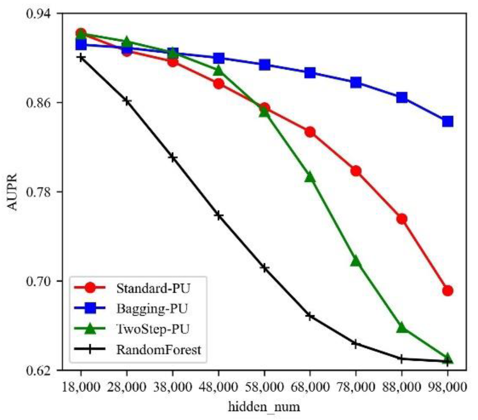
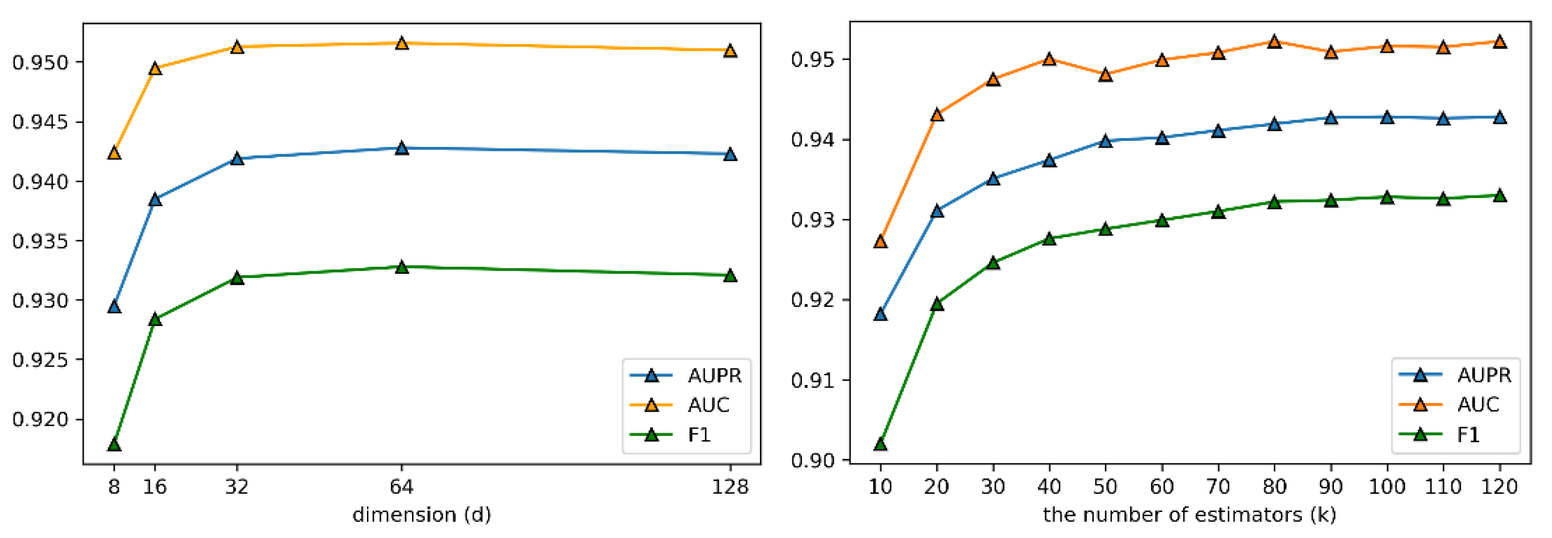
3.3. Parameter Analysis

It can be found that the Random Forest classifier performs best compared to other classifiers. Thus, in this section, we discuss the parameters in network representation and the Random Forest classifier.
There are two key parameters in our experiment: dimension of representation vector d and the number of estimators in the Random Forest classifier. We consider the combinations of parameters on the DrugBank dataset: d { 8 , 16 , 32 , 64 , 128 } , k { 10 , 20 , 30 , 40 , 50 , 60 , 70 , 80 , 90 , 100 , 110 , 120 } . We implement 3-CV to evaluate performances of our model with different parameter settings using AUPR and F1 metrics. Finally, we adopt d = 64 ,   k = 100 as the optimal parameters for our model in the following experiments.
We fix k = 100 to investigate the influence of d . In Figure 4 (Left), it can be seen that the performance of our model increases with the increase of the value of d , then decreases after reaching the peak ( d = 64 ). Then, we fix d = 64 to discuss the number of estimators k . As shown in Figure 4 (Right), the performance of our model increases as k increases from 10 to 100, followed by decreasing, and then reached the peak again when k = 120 . Our model obtains the best performance when k = 100 and k = 120 , but for reasonable time cost, we choose k = 100 as the optimal parameter.

4. Conclusions

In this paper, we present a positive-unlabeled learning framework with network representation for unlabeled learning from positive samples. We introduce three types of positive-unlabeled learning methods to improve predictive performances and design experiments to compare their contributions on different datasets for the network link prediction task. In our framework, the SDNE model is proven more effective to learn representations from network data than the other advanced models. Moreover, the PU learning methods can achieve good results, which are able to use the information in the unlabeled data set to help classifiers produce better performances. Among them, Standard-PU with Random Forest classifier achieves the best performance compared with other PU learning methods. the two-step method is the most commonly used PU learning technique, due to its conciseness and interpretability [12]. In addition, the Bagging PU learning method has also improved the effect of the classifier, but it is of less efficiency when the amount of data is large.
PU learning is a special case of standard semi-supervised learning, which is related to many areas of machine learning, such as single-class classification and learning with missing data. Given that PU data naturally appear in many real-world scenarios, PU learning will be a promising and active research direction in the field of machine learning in the future [48].

Author Contributions

Conceptualization, S.G. and S.L.; methodology, S.G.; software, S.L.; validation, S.G., M.A. and S.L.; formal analysis, S.G.; investigation, S.G.; resources, S.G. and S.L.; data curation, S.G.; writing—original draft preparation, S.G., M.A. and S.L.; writing—review and editing, S.G. and S.L.; visualization, S.G.; supervision, S.L.; project administration, S.L.; funding acquisition, S.G. All authors have read and agreed to the published version of the manuscript.

Funding

This work was supported by the National Natural Science Foundation of China (62102158), the Key projects of Hubei Provincial Department of Education (Q20203003), the Science and Technology Project of Hubei Province-Unveiling System (2019AEE020), and the 2020 Foshan support project for promoting the development of university scientific and technological achievements service industry (2020DZXX06). The funders have no role in study design, data collection, data analysis, data interpretation or writing of the manuscript.

Institutional Review Board Statement

Not applicable.

Informed Consent Statement

Not applicable.

Data Availability Statement

The datasets used in this paper are publicly available.

Conflicts of Interest

The authors declare no conflict of interest.

References

  1. Dong, Y.; Chawla, N.V.; Swami, A. metapath2vec: Scalable representation learning for heterogeneous networks. In Proceedings of the 23rd ACM SIGKDD International Conference on Knowledge Discovery and Data Mining, Halifax, NS, Canada, 13–17 August 2017; pp. 135–144. [Google Scholar]
  2. Nasiri, E.; Berahmand, K.; Samei, Z.; Li, Y. Impact of centrality measures on the common neighbors in link prediction for multiplex networks. Big Data 2022, 10, 138–150. [Google Scholar] [CrossRef]
  3. Nasiri, E.; Berahmand, K.; Li, Y. A new link prediction in multiplex networks using topologically biased random walks. Chaos Solitons Fractals 2021, 151, 111230. [Google Scholar] [CrossRef]
  4. Zamiri, M.; Yazdi, H.S. Image annotation based on multi-view robust spectral clustering. J. Vis. Commun. Image Represent. 2021, 74, 103003. [Google Scholar] [CrossRef]
  5. Fortunato, S. Community detection in graphs. Phys. Rep. 2010, 486, 75–174. [Google Scholar] [CrossRef]
  6. Tamassia, R. Handbook of Graph Drawing and Visualization; CRC Press: Boca Raton, FL, USA, 2013. [Google Scholar]
  7. Liben-Nowell, D.; Kleinberg, J. The link prediction problem for social networks. In Proceedings of the Twelfth International Conference on Information and Knowledge Management, New Orleans, LA, USA, 3–8 November 2003; pp. 556–559. [Google Scholar]
  8. Nasiri, E.; Berahmand, K.; Li, Y. Robust graph regularization nonnegative matrix factorization for link prediction in attributed networks. Multimed. Tools Appl. 2022, 1–24. [Google Scholar] [CrossRef]
  9. Martínez, V.; Berzal, F.; Cubero, J.C. A survey of link prediction in complex networks. ACM Comput. Surv. 2016, 49, 1–33. [Google Scholar] [CrossRef]
  10. Jaskie, K.; Spanias, A. Positive and unlabeled learning algorithms and applications: A survey. In Proceedings of the 2019 10th International Conference on Information, Intelligence, Systems and Applications (IISA), Patras, Greece, 15–17 July 2019; IEEE: Piscataway, NJ, USA, 2019; pp. 1–8. [Google Scholar]
  11. Bekker, J.; Davis, J. Estimating the class prior in positive and unlabeled data through decision tree induction. In Proceedings of the Thirty-Second AAAI Conference on Artificial Intelligence, New Orleans, LA, USA, 2–7 February 2018; Volume 32. [Google Scholar]
  12. Li, G. A survey on postive and unlabelled learning. Comput. Inf. Sci. 2013. [Google Scholar]
  13. Liu, B.; Dai, Y.; Li, X.; Lee, W.S.; Yu, P.S. Building text classifiers using positive and unlabeled examples. In Proceedings of the Third IEEE International Conference on Data Mining, Melbourne, FL, USA, 22–22 November 2003; IEEE: Piscataway, NJ, USA, 2003; pp. 179–186. [Google Scholar]
  14. Li, X.L.; Liu, B. Learning from positive and unlabeled examples with different data distributions. In European Conference on Machine Learning; Springer: Berlin/Heidelberg, Germany, 2005; pp. 218–229. [Google Scholar]
  15. Denis, F.; Gilleron, R.; Letouzey, F. Learning from positive and unlabeled examples. Theor. Comput. Sci. 2005, 348, 70–83. [Google Scholar] [CrossRef]
  16. Elkan, C.; Noto, K. Learning classifiers from only positive and unlabeled data. In Proceedings of the 14th ACM SIGKDD International Conference on Knowledge Discovery and Data Mining, Las Vegas, NV, USA, 24–27 August 2008; pp. 213–220. [Google Scholar]
  17. Mordelet, F.; Vert, J.P. A bagging SVM to learn from positive and unlabeled examples. Pattern Recognit. Lett. 2014, 37, 201–209. [Google Scholar] [CrossRef]
  18. Du Plessis, M.; Niu, G.; Sugiyama, M. Convex formulation for learning from positive and unlabeled data. In International Conference on Machine Learning; PMLR: Lille, France, 2015; pp. 1386–1394. [Google Scholar]
  19. Liu, B.; Lee, W.S.; Yu, P.S.; Li, X. Partially supervised classification of text documents. ICML 2002, 2, 387–394. [Google Scholar]
  20. Peng, T.; Zuo, W.; He, F. SVM based adaptive learning method for text classification from positive and unlabeled documents. Knowl. Inf. Syst. 2008, 16, 281–301. [Google Scholar] [CrossRef]
  21. Li, X.; Liu, B. Learning to classify texts using positive and unlabeled data. IJCAI 2003, 3, 587–592. [Google Scholar]
  22. Li, X.L.; Liu, B.; Ng, S.K. Negative training data can be harmful to text classification. In Proceedings of the 2010 Conference on Empirical Methods in Natural Language Processing, Cambridge, MA, USA, 9–11 October 2010; pp. 218–228. [Google Scholar]
  23. Lu, F.; Bai, Q. Semi-supervised text categorization with only a few positive and unlabeled documents. In Proceedings of the 2010 3rd International Conference on Biomedical Engineering and Informatics, Yantai, China, 16–18 October 2010; IEEE: Piscataway, NJ, USA, 2010; Volume 7, pp. 3075–3079. [Google Scholar]
  24. Kaboutari, A.; Bagherzadeh, J.; Kheradmand, F. An evaluation of two-step techniques for positive-unlabeled learning in text classification. Int. J. Comput. Appl. Technol. Res. 2014, 3, 592–594. [Google Scholar] [CrossRef]
  25. Lee, W.S.; Liu, B. Learning with positive and unlabeled examples using weighted logistic regression. ICML 2003, 3, 448–455. [Google Scholar]
  26. Khan, S.S.; Madden, M.G. One-class classification: Taxonomy of study and review of techniques. Knowl. Eng. Rev. 2014, 29, 345–374. [Google Scholar] [CrossRef]
  27. Chapelle, O.; Scholkopf, B.; Zien, A. Semi-Supervised Learning (Chapelle, O. et al., Eds.; 2006) [Book Reviews]. IEEE Trans. Neural Netw. 2009, 20, 542. [Google Scholar] [CrossRef]
  28. Manevitz, L.M.; Yousef, M. One-class SVMs for document classification. J. Mach. Learn. Res. 2001, 2, 139–154. [Google Scholar]
  29. Lü, L.; Zhou, T. Link prediction in complex networks: A survey. Phys. A Stat. Mech. Appl. 2011, 390, 1150–1170. [Google Scholar] [CrossRef]
  30. Goyal, P.; Ferrara, E. Graph embedding techniques, applications, and performance: A survey. Knowl.-Based Syst. 2018, 151, 78–94. [Google Scholar] [CrossRef]
  31. Grover, A.; Leskovec, J. node2vec: Scalable feature learning for networks. In Proceedings of the 22nd ACM SIGKDD International Conference on Knowledge Discovery and Data Mining, San Francisco, CA, USA, 13–17 August 2016; pp. 855–864. [Google Scholar]
  32. Ou, M.; Cui, P.; Pei, J.; Zhang, Z.; Zhu, W. Asymmetric transitivity preserving graph embedding. In Proceedings of the 22nd ACM SIGKDD International Conference on Knowledge Discovery and Data Mining, San Francisco, CA, USA, 13–17 August 2016; pp. 1105–1114. [Google Scholar]
  33. Tang, J.; Qu, M.; Wang, M.; Zhang, M.; Yan, J.; Mei, Q. Line: Large-scale information network embedding. In Proceedings of the 24th International Conference on World Wide Web, Florence, Italy, 18–22 May 2015; pp. 1067–1077. [Google Scholar]
  34. Wang, D.; Cui, P.; Zhu, W. Structural deep network embedding. In Proceedings of the 22nd ACM SIGKDD International Conference on Knowledge Discovery and Data Mining, San Francisco, CA, USA, 13–17 August 2016; pp. 1225–1234. [Google Scholar]
  35. Perozzi, B.; Al-Rfou, R.; Skiena, S. Deepwalk: Online learning of social representations. In Proceedings of the 20th ACM SIGKDD International Conference on Knowledge Discovery and Data Mining, New York, NY, USA, 24–27 August 2014; pp. 701–710. [Google Scholar]
  36. Liu, S.; Zhai, S.; Zhu, L.; Zhu, F.; Zhang, Z.M.; Zhang, W. Efficient network representations learning: An edge-centric perspective. In International Conference on Knowledge Science, Engineering and Management; Springer: Cham, Switzerland, 2019; pp. 373–388. [Google Scholar]
  37. Cen, Y.; Zou, X.; Zhang, J.; Yang, H.; Zhou, J.; Tang, J. Representation learning for attributed multiplex heterogeneous network. In Proceedings of the 25th ACM SIGKDD International Conference on Knowledge Discovery & Data Mining, Anchorage, AK, USA, 4–8 August 2019; pp. 1358–1368. [Google Scholar]
  38. Yang, C.; Xiao, Y.; Zhang, Y.; Sun, Y.; Han, J. Heterogeneous network representation learning: A unified framework with survey and benchmark. IEEE Trans. Knowl. Data Eng. 2020, 34, 4854–4873. [Google Scholar] [CrossRef]
  39. Dong, Y.; Hu, Z.; Wang, K.; Sun, Y.; Tang, J. Heterogeneous Network Representation Learning. IJCAI 2020, 20, 4861–4867. [Google Scholar]
  40. Xie, Y.; Yu, B.; Lv, S.; Zhang, C.; Wang, G.; Gong, M. A survey on heterogeneous network representation learning. Pattern Recognit. 2021, 116, 107936. [Google Scholar] [CrossRef]
  41. Cui, P.; Wang, X.; Pei, J.; Zhu, W. A survey on network embedding. IEEE Trans. Knowl. Data Eng. 2018, 31, 833–852. [Google Scholar] [CrossRef]
  42. Zhang, D.; Yin, J.; Zhu, X.; Zhang, C. Network representation learning: A survey. IEEE Trans. Big Data 2018, 6, 3–28. [Google Scholar] [CrossRef]
  43. Yu, H.; Han, J.; Chang, K.C.C. PEBL: Web page classification without negative examples. IEEE Trans. Knowl. Data Eng. 2004, 16, 70–81. [Google Scholar]
  44. Wishart, D.S.; Knox, C.; Guo, A.C.; Shrivastava, S.; Hassanali, M.; Stothard, P.; Chang, Z.; Woolsey, J. DrugBank: A comprehensive resource for in silico drug discovery and exploration. Nucleic Acids Res. 2006, 34 (Suppl. S1), D668–D672. [Google Scholar] [CrossRef]
  45. Zachary, W.W. An information flow model for conflict and fission in small groups. J. Anthropol. Res. 1977, 33, 452–473. [Google Scholar] [CrossRef] [Green Version]
  46. Sen, P.; Namata, G.; Bilgic, M.; Getoor, L.; Galligher, B.; Eliassi-Rad, T. Collective classification in network data. AI Mag. 2008, 29, 93. [Google Scholar] [CrossRef]
  47. Ahmed, A.; Shervashidze, N.; Narayanamurthy, S.; Josifovski, V.; Smola, A.J. Distributed large-scale natural graph factorization. In Proceedings of the 22nd International Conference on World Wide Web, Rio de Janeiro, Brazil, 13–17 May 2013; pp. 37–48. [Google Scholar]
  48. Bekker, J.; Davis, J. Learning from positive and unlabeled data: A survey. Mach. Learn. 2020, 109, 719–760. [Google Scholar] [CrossRef] [Green Version]
Figure 1. Traditional classifier learning and positive-unlabeled learning.
Mathematics 10 03345 g001
Figure 2. The architecture of our proposed framework consists of two modules: network representation module and positive-unlabeled learning module, as shown in (a). The positive-unlabeled learning module adopts three strategies to enhance the performance of predictive model (traditional classifier estimation is shown in (b), bagging strategy is shown in (c) and reliable negative sampling is shown in (d)).
Mathematics 10 03345 g002
Figure 3. The prediction performance of the positive-unlabeled learning methods with the increased number of empirical contaminations in the unlabeled set U.
Mathematics 10 03345 g003
Figure 4. Parameter Sensitivity of our method. (Left) The dimension of representation vector d, (Right) the number of estimators in the Random Forest classifier.
Mathematics 10 03345 g004
Table 1. The characteristics of the three experimental datasets.
DatasetNodeLinkAverage
Degree
Clustering
Coefficient
Assortativity
Coefficient
Type
DrugBank812165,802408.37930.6469−0.2031Bioinformatic network
Karate341569.17650.5706−0.4756Social network
Cora270810,5567.79620.2407−0.0659Citation network
Table 2. The performance of positive-unlabeled learning methods using different classifiers on the DrugBank dataset.
ClassifierMethodsAUPRAUCF1Accuracy
RFN/A0.88570.85270.82540.9246
Standard-PU0.93530.94710.92470.9624
Bagging-PU0.90850.95060.89990.9463
TwoStep-PU0.92100.93990.90970.9545
SVMN/A0.48420.61360.39180.7094
Standard-PU0.62300.54680.42880.3436
Bagging-PU0.62520.49930.40180.2514
TwoStep-PU0.57820.67830.51600.7129
LRN/A0.64650.62140.39610.8016
Standard-PU0.69020.78040.64190.7814
Bagging-PU0.69130.78170.64090.7765
TwoStep-PU0.68380.74630.57530.6519
DTN/A0.78150.77860.70120.8743
Standard-PU0.80560.82690.76190.8898
Bagging-PU0.90300.94520.89350.9430
TwoStep-PU0.82590.83450.77930.8997
NBN/A0.67860.76970.62880.7735
Standard-PU0.67890.77000.62840.7716
Bagging-PU0.67950.77050.62620.7650
TwoStep-PU0.68220.76940.61430.7345
Table 3. The performance of several network representation learning models using different positive-unlabeled learning strategies on the DrugBank dataset.
MethodsModelsAUPRAUCF1Accuracy
Standard-PUDeepwalk 0.8880 0.9252 0.8752 0.9350
GF0.79520.8597 0.7697 0.8752
Node2vec 0.8877 0.9268 0.8752 0.9345
LINE 0.9149 0.9281 0.8998 0.9505
SDNE0.93530.94710.92470.9624
Bagging-PUDeepwalk 0.8917 0.9378 0.8806 0.9357
GF 0.8090 0.8826 0.7831 0.8747
Node2vec 0.8905 0.9388 0.8793 0.9345
LINE 0.9051 0.9452 0.8958 0.9446
SDNE0.90850.95060.89990.9463
TwoStep-PUDeepwalk 0.8856 0.9049 0.8658 0.9340
GF 0.8017 0.8494 0.7736 0.8856
Node2vec 0.8860 0.9078 0.8675 0.9343
LINE 0.9082 0.92650.89370.9470
SDNE0.92100.93990.90970.9545
Table 4. The performance of different positive-unlabeled learning methods on three datasets.
DatasetMethodsAUPRAUCF1Accuracy
DrugBankRF0.88570.85270.82540.9246
Standard-PU(RF)0.93530.94710.92470.9624
Bagging-PU(RF)0.90850.95060.89990.9463
TwoStep-PU(RF)0.92100.93990.90970.9545
KarateRF0.62260.61700.37590.8904
Standard-PU(RF)0.67450.84290.62810.8681
Bagging-PU(RF)0.63440.82150.55060.8119
TwoStep-PU(RF)0.65270.78840.62030.8841
CoraRF0.58100.56870.24140.9566
Standard-PU(RF)0.59260.82020.56970.9487
Bagging-PU(RF)0.52670.83500.34300.8409
TwoStep-PU(RF)0.51550.73720.50260.9504
Publisher’s Note: MDPI stays neutral with regard to jurisdictional claims in published maps and institutional affiliations.

