Portfolio Insurance through Error-Correction Neural Networks

Abstract

Minimum-cost portfolio insurance (MCPI) is a well-known investment strategy that tries to limit the losses a portfolio may incur as stocks decrease in price without requiring the portfolio manager to sell those stocks. In this research, we define and study the time-varying MCPI problem as a time-varying linear programming problem. More precisely, using real-world datasets, three different error-correction neural networks are employed to address this financial time-varying linear programming problem in continuous-time. These neural network solvers are the zeroing neural network (ZNN), the linear-variational-inequality primal-dual neural network (LVI-PDNN), and the simplified LVI-PDNN (S-LVI-PDNN). The neural network solvers are tested using real-world data on portfolios of up to 20 stocks, and the results show that they are capable of solving the financial problem efficiently, in some cases more than five times faster than traditional methods, though their accuracy declines as the size of the portfolio increases. This demonstrates the speed and accuracy of neural network solvers, showing their superiority over traditional methods in moderate-size portfolios. To promote and contend the outcomes of this research, we created two MATLAB repositories, for the interested user, that are publicly accessible on GitHub.

1. Introduction and Motivation

The effects of the severe financial crisis that occurred in 2008 have characterized financial markets in recent years, followed by the associated rise in equity markets and associated decline in interest rate levels globally, up until a significant market decline in 2018 and the extremely volatile market conditions brought on by the COVID-19 crisis in the first quarter of 2020. Such a scenario suggests that it will always be difficult to predict how asset prices will behave and to make the appropriate countermoves in order to later create appropriate portfolio strategies in accordance with certain risk profiles. In these types of scenarios, portfolio insurance strategies such as guarantee funds and variable annuities are frequently used to provide investors with the promised assurances. Portfolio insurance’s primary goal is to limit a portfolio’s downside risk while maintaining its maximum return potential. A number of portfolio insurance optimization strategies have been proposed in recent years, using a variety of computational techniques, such as Riesz space-based techniques [1,2] and metaheuristics [3,4,5]. More specifically, the authors considered a linear programming portfolio insurance problem in [1,2], an integer programming portfolio insurance problem in [3], and a nonlinear programming multiperiod portfolio insurance problem under transaction costs in [4,5].

Recently, neural network (NN) techniques, such as weights- and structure-determination-based NNs [6,7], collaborative neurodynamic optimization [8], nonlinear NNs [9], and reinforcement learning [10], have been utilized to address portfolio optimization. A number of portfolio optimization strategies through NNs have been proposed in the past, such as predicting the distribution of a financial quantity [11], predicting the portfolio Sharpe ratio [12], and integrating the return prediction of traditional time series models in portfolio formation [13]. In general, there are two ways to apply NNs to portfolio construction: limiting loss [1,4,5] and seeking profit [11,12,13]. This work focuses on limiting portfolio loss. It defines and explores a time-varying variation of the minimum-cost portfolio insurance (MCPI) problem as a time-varying linear programming (TLP) problem. More precisely, using real-world datasets, three different error-correction NNs (ENNs) are employed to address the financial TLP problem in continuous-time (CT). These NN solvers are the zeroing NN (ZNN), the linear-variational-inequality primal-dual NN (LVI-PDNN), and the simplified LVI-PDNN (S-LVI-PDNN). When it comes to solving TLP problems, such as the time-varying MCPI (TMCPI) problem, the ZNN approach is comparable to the LVI-PDNN and S-LVI-PDNN methods because they are all based on the error-correction principle.

The ZNN framework was created by Zhang et al. in [14] for generating online solutions to time-varying (TV) problems and it is based on the Hopfield neural network. Notice that the vast majority of ZNN-based dynamical systems, as well as the LVI-PDNN and S-LVI-PDNN, are classified as recurrent NNs (RNNs), which are utilized to locate equations’ zeros. On the one hand, the ZNN approach has been extensively used in a variety of time-varying topics, with the most common being problems of generalized inversion [15,16], matrix equations systems [17,18], quadratic optimization [19,20], linear equations systems [17], and various matrix functions approximation [21,22]. On the other hand, the LVI-PDNN is widely employed in robotic applications, such as the construction of mobile robots’ vision-related control systems [23] or resolution of kinematic redundancy in robot manipulators [24], and it has recently been successfully used in solving financial problems such as asset portfolio selection [20]. As a result, this article’s primary goal is to efficiently solve the TMCPI problem through ENN methods (i.e., ZNN, LVI-PDNN, and S-LVI-PDNN).

The primary advantages of employing an artificial NN include generalization, fault and noise tolerance, and the capacity to predict data that have not yet been seen while saving costs and time [21]. Based on our previous experience with portfolio selection problems, we apply the advantages of ENN solvers (i.e., ZNN, LVI-PDNN, and S-LVI-PDNN) to solve the TMCPI problem within a realistic framework of financial portfolio management. Furthermore, as is well known, ENN solvers can be viewed as predictive dynamics. By employing these ENN methods, the proposed models in [15,19] achieve excellent convergence performance, while the convergence speed can be changed by altering the design parameter [21]. As a consequence, by using the ZNN, LVI-PDNN, and S-LVI-PDNN methods, the TMCPI problem can be addressed with exponential convergence performance. To be able to track the evolution of the static MCPI problem over time and to offer a form of prediction, we investigate the TMCPI problem as a continuous TLP problem.

The main contributions of this work can be summed up as follows:

• The TMCPI problem is defined and explored;
• Three novel ENN models for addressing the TMCPI problem are defined;
• We use ENN solvers on real-world datasets;
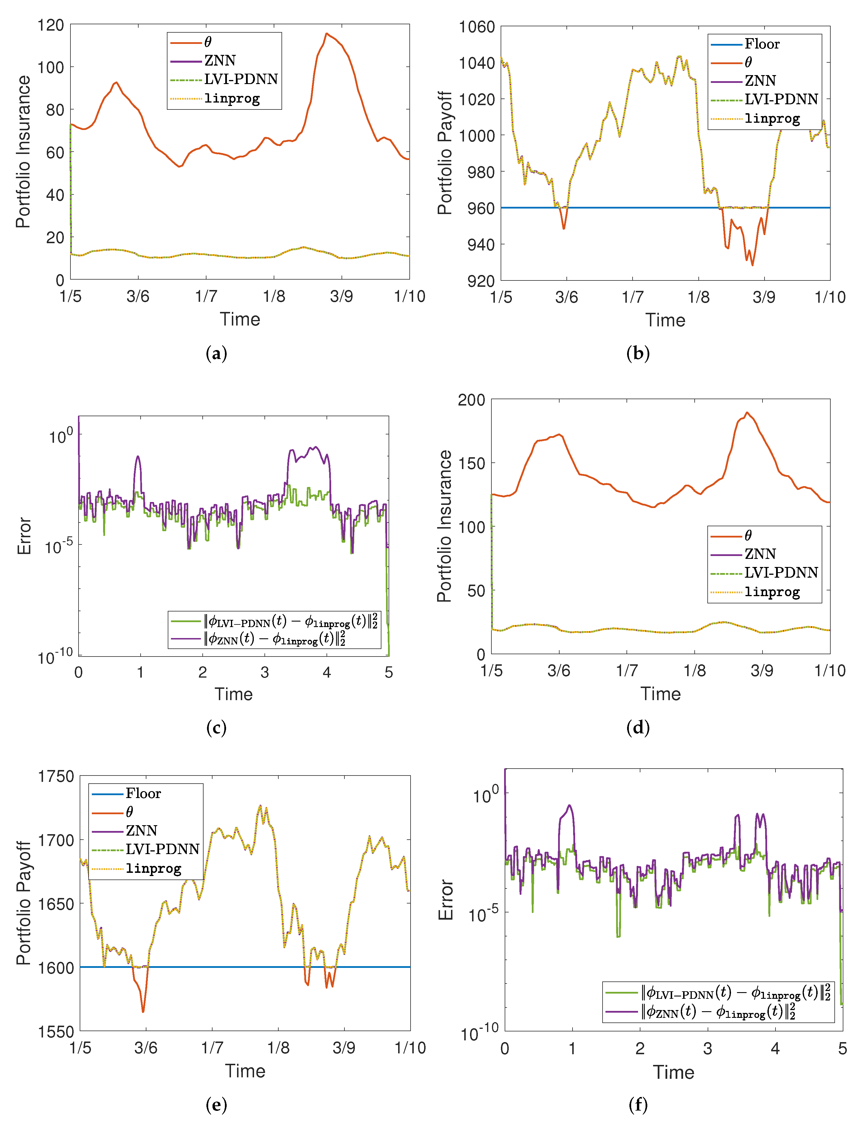
• The performance of the ENN solvers versus the conventional MATLAB solver is demonstrated and contrasted in trials using four different portfolio configurations.

The following hierarchy governs the overall organization of the document’s sections. The TV variation of the MCPI problem is introduced in Section 2. Section 3 presents the ENN solvers. Experiments in Section 4 highlight the performance and efficacy of the ENN solvers for solving the TMCPI problem in four different portfolio setup cases using daily real-world data. Additionally, information about a publicly accessible MATLAB repository on GitHub is provided in Section 4. This repository implements all of the techniques and procedures outlined in Section 3 and Section 4 to promote the readability and computational value of this research. The conclusions section is Section 5.

2. Minimum-Cost Portfolio Insurance

In many situations, portfolio insurance solutions are employed to give investors promised guarantees [1,25,26]. The past literature has proposed a wide range of portfolio insurance strategies, some of which have been expanded to the dynamic setting. This section introduces a continuous-time portfolio insurance approach as an innovative technique that integrates robust processes from ENNs to provide online, thus more realistic, solutions.

TV Variation of the MCPI Problem

Reducing portfolio costs is always a priority for financial engineers. The obvious way to reduce portfolio costs is to reduce insurance costs (see [3,4]). Here, we present a TV analog of the corresponding portfolio insurance static problem, which has been described and investigated in a number of papers, including [2,27].

Note that, when we say a vector $d\left(t\right)\in {\mathbb{R}}^n$ or a matrix $D\left(t\right)\in {\mathbb{R}}^{m\times n}$, we mean a vector or a matrix that change over time t, and also, ${(·)}^{\mathrm{T}}$ denotes matrix transposition. Assume the market $X\left(t\right)={[x_1\left(t\right),x_2\left(t\right),\dots ,x_n\left(t\right)]}^T\in {\mathbb{R}}^n$ at time $t=1,2,\dots ,\mu$, where $x_i\left(t\right)\in \mathbb{R}$ is the asset’s i, $i=1,2,\dots ,n$, return, and the initial portfolio $\theta ={[{\theta }_1,{\theta }_2,\dots ,{\theta }_n]}^T\in {\mathbb{R}}^n$, where ${\theta }_i$, $i=1,2,\dots ,n$, is the ith asset. Then, the payoff of a portfolio $\theta$ is given by the formula

$$X^{\mathrm{T}}\left(t\right)·\theta$$

(1)

Additionally, assume the insurance prices $p\left(t\right)={[p_1\left(t\right),p_2\left(t\right),\dots ,p_n\left(t\right)]}^T\in {\mathbb{R}}^n$ where $p_i\left(t\right)\in \mathbb{R}$ is the asset’s i, $i=1,2,\dots ,n$, insurance price. In our case, we assume that the portfolio’s insurance costs include a standard price plus an asset risk rate. The function of the fixed and linear insurance prices is made up as follows if the price rates connected to asset risk are denoted by $\delta$ and the fixed price by $\beta$:

$$p_i\left(t\right)=\beta +\delta ·\mathrm{Var}\left[\frac{Y_i\left(t\right)}{max\left(Y_i\left(t\right)\right)}\right],i=1,2,\dots ,n,$$

(2)

where $Y_i\left(t\right)={[x_i\left(t\right),x_i(t-1),\dots ,x_i(t-\tau +1)]}^T$ and $\mathrm{Var}\left[Y_i\left(t\right)\right]$ denotes the variance of $Y_i\left(t\right)$. The number $\tau \le t-1$, $\tau \in \mathbb{N}$, is constant and implies the time delays. Since $Y_i\left(t\right)\in {\mathbb{R}}^{\tau }$, the risk of the i asset is determined by the variance of $\tau$ normalized prices. In this way, any asset’s insurance cost is based on the amount of risk it carries, where there is a chance that the predicted return will differ from the actual return. As a result, insurance prices are rising in line with inflation.

It is important to mention that the insured payoff of the portfolio $\theta$, under the floor price $k\in \mathbb{R}$ and the price $p\left(t\right)$, is the maximum between the payoff of $\theta$ and k, i.e., $max\{X^{\mathrm{T}}\left(t\right)·\theta ,k\}$. Consequently, given an initial portfolio $\theta$ and a floor price k, the TLP formulation of the TMCPI problem is as below:

$$\begin{array}{ccc}& \underset{\varphi \left(t\right)}{min}& p^{\mathrm{T}}\left(t\right)·\varphi \left(t\right)\hfill \end{array}$$

(3)

$$\begin{array}{ccc}& \mathrm{s}.\mathrm{t}.& -X^{\mathrm{T}}\left(t\right)·\varphi \left(t\right)\le min\{-X^{\mathrm{T}}\left(t\right)·\theta ,-k\}\hfill \end{array}$$

(4)

$$\begin{array}{ccc}& & 0\le \varphi \left(t\right)\le \zeta \left(t\right),\hfill \end{array}$$

(5)

where $\varphi \left(t\right)={[{\varphi }_1\left(t\right),{\varphi }_2\left(t\right),\dots ,{\varphi }_n\left(t\right)]}^T\in {\mathbb{R}}^n$ is the optimal insured portfolio, $\zeta \left(t\right)=X^{\mathrm{T}}\left(t\right)·\theta ·{\left[\frac{1}{x_1\left(t\right)},\dots ,\frac{1}{x_n\left(t\right)}\right]}^T\in {\mathbb{R}}^n$, and the right part of (5), i.e., $\zeta \left(t\right)$, is the maximum merit of each stock that an investor is allowed to keep at time t, by investing in each of them all the portfolio’s $\theta$ payoff.

Moreover, by interpolating $X\left(t\right)$ and $p\left(t\right)$ into continuous functions, we transform the TMCPI problem from discrete-time (DT) to CT. As a result, considering the space of all continuous real functions $C[0,\mu -\tau -1]$ on the closed interval $[0,\mu -\tau -1]$, we have that $X\left(t\right),p\left(t\right)\in C[0,\mu -\tau -1]$, and $\varphi \left(t\right)$ becomes the online solution of the TMCPI problem (3)–(5).

3. The Error-Correction Neural Network Approach

Bearing in mind its basic role in mathematical optimization, most aspects of linear programming (LP) have been thoroughly studied over the last decades. Solutions to LP problems have been commonly used in a wide range of research and industrial applications; see for example [28,29]. In the past, typically fewer than two different types of constraints have been subject to LP problems; see for example [30]. Most studies were dedicated to the so-called static LP problems, see [31], which means that methods and algorithms designed to address such a group of LP problems are inoperative when employed to TV situations. The ZNN, LVI-PDNN, and S-LVI-PDNN are three types of ENNs that are specifically designed to zeroing time-varying equations, which have been critical in solving a variety of difficult TV problems in various scientific domains [20,21]. This section describes the ENN solvers for approaching the TMCPI problem of (3)–(5).

In what follows, we denote by $\mathbf{1}$ and $\mathbf{0}$, respectively, those vectors of ${\mathbb{R}}^n$ containing ones and zeros; $I_n$ for the identity $n\times n$ matrix; and ${\mathbf{0}}_{m\times k}$ for the zero $m\times k$ matrix; ⊙ signifies the element-wise (or Hadamard) product and ${\left(\right)}^{\odot }$ the element-wise exponential; and a square diagonal matrix with the components of the vector x on the main diagonal is denoted by $\overline{x}$.

3.1. TMCPI Problem via ZNN

Since its introduction by Zhang et al. in 2001 [32], the ZNN evolution has been studied and developed as a significant class of recurrent NNs. The theoretical investigation of ZNNs has shown that they are a powerful tool for solving TV problems. According to the ZNN’s design, under the linear activation function, we define an error matrix $K\left(t\right)$ which can be dynamically controlled using the formula [18]:

$$\dot{K}\left(t\right)=-\gamma K\left(t\right),$$

(6)

where $\gamma >0$ is the design parameter and $\dot{\left(\right)}$ signifies the time derivative. $K\left(t\right)$ is forced to exponentially converge to the zero matrix by (6), and also, as the value of $\gamma$ increases the convergence rate increases, too. The three steps listed below can be used to achieve our goal of developing a ZNN model in line with the Karush–Kuhn–Tucker (KKT) conditions [33,34] to solve the TMCPI problem.

• Step 1:(TMCPI problem reformulation) The TMCPI problem of (3)–(5) can be reformulated as follows:

  $$\begin{array}{ccc}& \underset{\varphi \left(t\right)}{min}& p^{\mathrm{T}}\left(t\right)·\varphi \left(t\right)\hfill \end{array}$$

  (7)

  $$\begin{array}{ccc}& \mathrm{s}.\mathrm{t}.& -X^{\mathrm{T}}\left(t\right)·\varphi \left(t\right)\le min\{-X^{\mathrm{T}}\left(t\right)·\theta ,-k\}\hfill \end{array}$$

  (8)

  $$\begin{array}{ccc}& & \varphi \left(t\right)\le \zeta \left(t\right)\hfill \end{array}$$

  (9)

  $$\begin{array}{ccc}& & -\varphi \left(t\right)\le \mathbf{0},\hfill \end{array}$$

  (10)

  or equivalently

  $$\begin{array}{cc}\hfill \underset{\varphi \left(t\right)}{min}& p^{\mathrm{T}}\left(t\right)·\varphi \left(t\right)\end{array}$$

  (11)

  $$\begin{array}{cc}\hfill \mathrm{s}.\mathrm{t}.& A\left(t\right)\varphi \left(t\right)\le b\left(t\right),\end{array}$$

  (12)

  where $A\left(t\right)=\left[\begin{array}{c}-X^{\mathrm{T}}\left(t\right)\\ I_n\\ -I_n\end{array}\right]\in {\mathbb{R}}^{(2n+1)\times n}$ and $b\left(t\right)=\left[\begin{array}{c}min\{-X^{\mathrm{T}}\left(t\right)·\theta ,-k\}\\ \zeta \left(t\right)\\ \mathbf{0}\end{array}\right]\in {\mathbb{R}}^{2n+1}$.
• Step 2:(Minimization conditions) To address the TLP problem of (11)–(12), the following Lagrange function is defined:

  $$L(\varphi \left(t\right),\lambda \left(t\right),R\left(t\right),t)=p^{\mathrm{T}}\left(t\right)\varphi \left(t\right)+{\lambda }^{\mathrm{T}}\left(t\right)(A\left(t\right)\varphi \left(t\right)+R^{\odot 2}\left(t\right)-b\left(t\right)),$$

  (13)

  where $\lambda \left(t\right)\in {\mathbb{R}}^{2n+1}$ and $R^{\odot 2}\left(t\right)\in {\mathbb{R}}^{2n+1}$ is a non-negative time-varying term that converts the inequality constraint to an equality constraint. Then, using the KKT conditions [35], we have

  $$\left\{\begin{array}{c}\frac{\partial L\left(\varphi \right(t),\lambda (t),R(t),t)}{\partial \varphi \left(t\right)}=p\left(t\right)+A^{\mathrm{T}}\left(t\right)\lambda \left(t\right)=0\hfill \\ \frac{\partial L\left(\varphi \right(t),\lambda (t),R(t),t)}{\partial \lambda \left(t\right)}=A\left(t\right)\varphi \left(t\right)+R^{\odot 2}\left(t\right)-b\left(t\right)=0\hfill \\ \frac{\partial L\left(\varphi \right(t),\lambda (t),R(t),t)}{\partial R\left(t\right)}=\lambda \left(t\right)\odot R\left(t\right)=0\hfill \end{array}\right.$$

  (14)
• Step 3:(ZNN method) Considering the next equation group of error matrices

  $$\left\{\begin{array}{c}{K}_1\left(t\right)=p\left(t\right)+A^{\mathrm{T}}\left(t\right)\lambda \left(t\right)\hfill \\ K_2\left(t\right)=A\left(t\right)\varphi \left(t\right)+R^{\odot 2}\left(t\right)-b\left(t\right)\hfill \\ K_3\left(t\right)=\lambda \left(t\right)\odot R\left(t\right)\hfill \end{array}\right.$$

  (15)

  and then substituting $K_i\left(t\right),i=1,2,3,$ defined in (15) in place of $E\left(t\right)$ into (6), one obtains

  $$\left\{\begin{array}{c}\dot{p}\left(t\right)+A^{\mathrm{T}}\left(t\right)\dot{\lambda }\left(t\right)+{\dot{A}}^{\mathrm{T}}\left(t\right)\lambda \left(t\right)=-\gamma K_1\left(t\right)\hfill \\ \dot{A}\left(t\right)\varphi \left(t\right)+A\left(t\right)\dot{\varphi }\left(t\right)+2R\left(t\right)\dot{R}\left(t\right)-\dot{b}\left(t\right)=-\gamma K_2\left(t\right)\hfill \\ \dot{\lambda }\left(t\right)R\left(t\right)+\lambda \left(t\right)\dot{R}\left(t\right)=-\gamma K_3\left(t\right)\hfill \end{array}\right.$$

  (16)

  where,

  $$\dot{A}\left(t\right)=\left[\begin{array}{c}-{\dot{X}}^{\mathrm{T}}\left(t\right)\\ \mathbf{0}\\ \mathbf{0}\end{array}\right]\in {\mathbb{R}}^{(2n+1)\times n},\dot{b}\left(t\right)=\left[\begin{array}{c}min\{-{\dot{X}}^T\left(t\right)·\theta ,0\}\\ \dot{\zeta }\left(t\right)\\ \mathbf{0}\end{array}\right]\in {\mathbb{R}}^{2n+1}$$

  (17)

Then setting

$$\begin{gathered} S\left(t\right)=\left[\begin{array}{ccc}{\mathbf{0}}_{n\times n}& A^{\mathrm{T}}\left(t\right)& {\mathbf{0}}_{n\times (2n+1)}\\ A\left(t\right)& {\mathbf{0}}_{(2n+1)\times (2n+1)}& 2\overline{R}\left(t\right)\\ {\mathbf{0}}_{(2n+1)\times n}& \overline{R}\left(t\right)& \overline{\lambda }\left(t\right)\end{array}\right], \\ u\left(t\right)=\left[\begin{array}{c}-\gamma K_1\left(t\right)-\dot{p}\left(t\right)-{\dot{A}}^{\mathrm{T}}\left(t\right)\lambda \left(t\right)\\ -\gamma K_2\left(t\right)-\dot{A}\left(t\right)x\left(t\right)+\dot{b}\left(t\right)\\ -\gamma K_3\left(t\right)\end{array}\right], \end{gathered}$$

(18)

where $S\left(t\right)\in {\mathbb{R}}^{(5n+2)\times (5n+2)}$ and $u\left(t\right)\in {\mathbb{R}}^{5n+2}$, (16) can be reformulated as follows:

$$S\left(t\right)\dot{y}\left(t\right)=u\left(t\right),$$

(19)

where $\dot{y}\left(t\right)=\left[\begin{array}{c}\dot{\varphi }\left(t\right)\\ \dot{\lambda }\left(t\right)\\ \dot{R}\left(t\right)\end{array}\right]\in {\mathbb{R}}^{5n+2}$ and $S\left(t\right)$ acts as the corresponding mass matrix. The model of (19) is adequate for addressing the TLP problem of (3)–(5). The solution to (19) is given by:

$$\dot{y}\left(t\right)={\left(S^T\left(t\right)S\left(t\right)\right)}^{†}{S}^T\left(t\right)u\left(t\right),$$

(20)

where ${(·)}^{†}$ denotes the Moore–Penrose inverse. To establish that the ZNN solver converges to the theoretical solution, we give the following theorem.

Theorem 1.

The state vector $y\left(t\right)={\left[\varphi \left(t\right),\lambda \left(t\right),R\left(t\right)\right]}^{\mathrm{T}}$ of a ZNN (20) converges universally to the theoretical solution $y^{*}\left(t\right)={\left[{\varphi }^{*}\left(t\right),{\lambda }^{*}\left(t\right),R^{*}\left(t\right)\right]}^{\mathrm{T}}$ starting from any initial condition $y\left(0\right)\in {\mathbb{R}}^{5n+2}$. To put it another way, $\underset{t\to \infty }{lim}(y\left(t\right)-y^{*}\left(t\right))=0$, while the first n components of $y^{*}\left(t\right)$ are the theoretical solution ${\varphi }^{*}\left(t\right)$ of the optimization problem in (3)–(5).

Proof. 

The error matrix equation group is determined as in (15), in line with the ZNN architecture, to achieve the solution $\varphi \left(t\right)$ of TLP (3)–(5). The model (16) is then obtained by using the linear design formula for zeroing (15). When $t\to \infty$, each error matrix equation in the group (16) converges to the zero matrix, according to [14] (Theorem 1). As a consequence, when $t\to \infty$, the solution $y\left(t\right)$ of (16) converges to the theoretical solution $y^{*}\left(t\right)$ of TLP (4)–(5). Additionally, we can infer from the (20) derivation procedure that it is merely a variant of the (16) error. Thus, the proof is finished.    □

3.2. TMCPI Problem via LVI-PDNN and S-LVI-PDNN

In this section, we discuss two ENN solvers, the LVI-PDNN and the S-LVI-PDNN, both developed by Zhang et al. [36]. The LVI-PDNN may solve online (3)–(5), by setting

$$S\left(t\right)=\left[\begin{array}{cc}{\mathbf{0}}_{n\times n}& -X\left(t\right)\\ X^{\mathrm{T}}\left(t\right)& 0\end{array}\right]\in {\mathbb{R}}^{(n+1)\times (n+1)},v\left(t\right)=\left[\begin{array}{c}p\left(t\right)\\ min\left\{A\right(t)·\theta ,-k\}\end{array}\right]\in {\mathbb{R}}^{n+1},$$

(21)

where $w\left(t\right)$ is the primal dual-decision vector and the lower and higher boundaries in (5) are as below:

$$w\left(t\right)=\left[\begin{array}{c}\varphi \left(t\right)\\ c\left(t\right)\end{array}\right]\in {\mathbb{R}}^{n+1},{\rho }^{-}\left(t\right)=\left[\begin{array}{c}\mathbf{0}\\ 0\end{array}\right]\in {\mathbb{R}}^{n+1},{\rho }^{+}\left(t\right)=\left[\begin{array}{c}\zeta \left(t\right)\\ 1e+100\end{array}\right]\in {\mathbb{R}}^{n+1},$$

(22)

The $c\left(t\right)\in \mathbb{R}$ denotes the dual-decision vector of inequality constraint (4), while $\varphi \left(t\right)$ is the decision parameter of (5).

The following dynamical model, known as the LVI-PDNN, can be used to solve the TMCPI problem of (3)–(5):

$$\dot{w}\left(t\right)=\gamma (I_{n+1}+S^{\mathrm{T}}\left(t\right))(\Psi (w\left(t\right)-(S\left(t\right)w\left(t\right)+v\left(t\right)))-w\left(t\right)),$$

(23)

where $\gamma >0$ signifies the design parameter and the projection operator is the following element-wise function:

$${\Psi }_i\left(w_i\left(t\right)\right)=\left\{\begin{array}{cc}{\rho }_i^{-}\left(t\right),\hfill & w_i\left(t\right)<{\rho }_i^{-}\left(t\right)\hfill \\ w_i\left(t\right),\hfill & {\rho }_i^{-}\left(t\right)\le w_i\left(t\right)\le {\rho }_i^{+}\left(t\right),\hfill \\ {\rho }_i^{+}\left(t\right),\hfill & w_i\left(t\right)>{\rho }_i^{+}\left(t\right)\hfill \end{array}\right.\mathrm{for}i=1,2,...,2+n.$$

(24)

The price of $\gamma$ must be set to the greatest possible value or selected appropriately within hardware constraints for experimental or simulation purposes. It should be noted that a MATLAB ode solver can be used to effectively produce the solution $w\left(t\right)$ of (23).

The simplified version of the LVI-PDNN, called the S-LVI-PDNN, is the following dynamical model:

$$\dot{w}\left(t\right)=\gamma (\Psi (w\left(t\right)-(S\left(t\right)w\left(t\right)+v\left(t\right)))-w\left(t\right)),$$

(25)

which can also be used to solve the TMCPI problem of (3)–(5).

To better understand the real-time convergence of the LVI-PDNN and S-LVI-PDNN, the residual error is calculated as bellow:

$$K\left(t\right)=w\left(t\right)-\Psi \left(w\right(t)-(S\left(t\right)w\left(t\right)+v\left(t\right)\left)\right).$$

(26)

According to [36] (Theorems 1 and 2) and [37] (Theorem 3), if ${∥K\left(t\right)∥}_2^2\to 0$, the convergence of the state vector $w\left(t\right)$ to the optimal solution $w^{*}\left(t\right)$ can be accomplished, and thus the LVI-PDNN and S-LVI-PDNN converge to the theoretical solution.

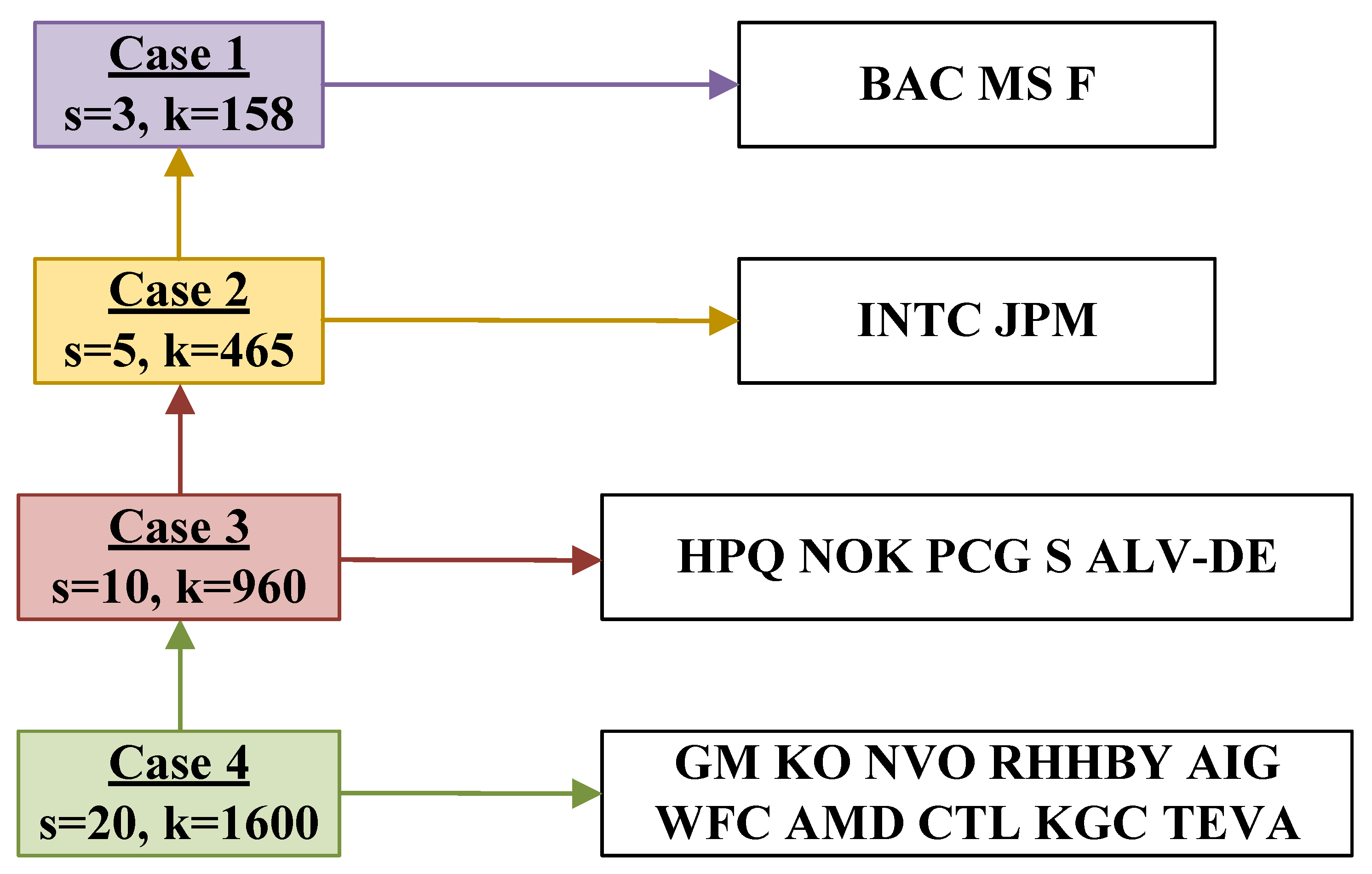
4. Real-World Experiments

We use the time series of portfolio returns and insurance prices as input, so the data are in DT. To solve a CT problem and provide an online solution, we must first convert the input data from DT to CT. We accomplish this by employing interpolation functions on $X\left(t\right),\dot{X}\left(t\right),p\left(t\right)$, and $\dot{p}\left(t\right)$. It is worth mentioning that the time derivatives of $\zeta \left(t\right)$, $X\left(t\right)$, and $p\left(t\right)$ can be created by setting $\dot{\zeta }\left(t\right)=\zeta (t+1)-\zeta \left(t\right)$, $\dot{X}\left(t\right)=X(t+1)-X\left(t\right)$ and $\dot{p}\left(t\right)=p(t+1)-p\left(t\right)$, respectively. Here, we apply linear interpolation to the DT data we have. To accomplish this, we use the MATLAB custom function linots, which is retrieved from [38]. That is, the DT arrays $X\left(t\right),\dot{X}\left(t\right),p\left(t\right)$, and $\dot{p}\left(t\right)$ are converted into interpolated CT functions using linots. A number of alternative interpolation techniques can be found in [38]. Their major benefit, over commercial MathWorks functions, is that they are designed to reduce the computational costs of the MATLAB ode solvers we used. Therefore, when time series constitute the input data, the ENNs produce quicker results.

Moreover, the ode15s MATLAB solver is employed in (20), (23), and (25) to generate the online solution of the TMCPI problem with the parameters set to $\gamma =1e3$, $\beta =2$, and $\delta =1e3$. The financial time series are obtained from https://finance.yahoo.com, accessed on 10 August 2022. The following GitHub link leads to the entire implementation and development of the TMCPI problem discussed in Section 3 and Section 4: https://github.com/SDMourtas/TMCPI, accessed on 10 August 2022. Lastly, the solutions provided by the ZNN, LVI-PDNN, and S-LVI-PDNN are contrasted to the presumptive theoretical solutions produced by the MATLAB function linprog. It is worth mentioning that all numerical experiments are performed using the MATLAB R2021a environment on an ${\mathrm{Intel}}^{\circledR }$${\mathrm{Core}}^{\mathrm{TM}}$ i5-6600K CPU 3.50 GHz, 16 GB RAM, running on a Windows 10 64-bit Operating System.

Portfolio Cases

Four alternative portfolio setup cases are covered by the trials. In Figure 1, the portfolio cases are shown, with the portfolios’ market including stocks that are among the most active on the US market. In the i-th case, $i=1,2,3,4$, we consider the market $X=[x_1,x_2,\dots ,x_s]$, where X includes the daily close prices of the s stocks shown in Figure 1, for the time period 2 April 2019 to 1 October 2019. It is worth noting that s includes all stocks from the beginning until the case of interest, so case two, for example, includes BAC, MS, F, INTC, and JPM. Setting the time delay parameter $\tau =21$ for calculating the insurance prices, we try to find through ENNs the optimal portfolio $\varphi \left(t\right)$ for the time period 1 May 2019 to 1 October 2019. It is important to note that for solving the omitted recorded prices problem between periods of the same division, we utilize the parameter $\omega$ from [38], which splits the recorded prices to the time periods for each t inside the ZNN, LVI-PDNN, and S-LVI-PDNN. More precisely, we set

$$\omega =\left\{\begin{array}{cc}22\hfill & ,t\in [0,1)\hfill \\ (22+20·(t-1\left)\right)/t\hfill & ,t\in [1,2)\hfill \\ (42+22·(t-2\left)\right)/t\hfill & ,t\in [2,4)\hfill \\ (86+21·(t-4\left)\right)/t\hfill & ,t\in [4,5]\hfill \end{array}\right.$$

which separates the time series from 1 May 2019 to 1 October 2019 into five monthly intervals. Then, we employ $X\left(\omega t\right)$ and $p\left(\omega t\right)$ instead of $X\left(t\right)$ and $p\left(t\right)$ and $\dot{X}\left(\omega t\right)$ and $\dot{p}\left(\omega t\right)$ instead of $\dot{X}\left(t\right)$ and $\dot{p}\left(t\right)$. As a result, we set $tspan=[0,5]$ in the MATLAB ode15s solver to find the optimal portfolio $\varphi \left(t\right)$ for the time period 1 May 2019 to 1 October 2019. Given an initial portfolio $\theta =2$ones$(s,1)$ and a floor k, and starting from $y\left(0\right)=[\theta ;2$ones$(4s+2,1)]$ in (20) and $w\left(0\right)=[\theta ;2]$ in (23) and (25), the results are presented in Figure 2 and Figure 3.

For the portfolio cases 1 and 2, which deal with three- and five-stock portfolios, respectively, Figure 2a,e show the weights of the optimal insured portfolio $\varphi \left(t\right)$ generated by the ZNN, LVI-PDNN, S-LVI-PDNN, and linprog. In Figure 2a, we can see that all of the portfolios in case 1 are identical with the exception of the portfolio generated by the ZNN, which is slightly different, whereas in Figure 2e, we can see that only the portfolios of the LVI-PDNN and linprog in case 2 are identical with the remainder being marginally different. Figure 2b,f show the insurance costs incurred by each portfolio, i.e., the initial portfolio $\theta$ and the portfolios $\varphi \left(t\right)$ generated by the ZNN, LVI-PDNN, S-LVI-PDNN, and linprog. We can see that the portfolios in cases 1 and 2 are almost identical. Figure 2c,g show the payoff of each portfolio $\varphi \left(t\right)$ along with the floor price k. Then, the portfolios in cases 1 and 2 are identical with the exception of the portfolio generated by the S-LVI-PDNN, which is marginally different and begins to become excessively noisy in Figure 2g of case 2. The errors between the solutions of linprog and the ENNs, which are presented in Figure 2d,h for cases 1 and 2, respectively, can support the aforementioned. That is, while the S-LVI-PDNN accuracy declines significantly as the problem’s dimensions rise, the LVI-PDNN has the same convergence rate and marginally higher accuracy than the ZNN. As a result, the S-LVI-PDNN method has been left out for portfolio cases 3 and 4, which deal with larger portfolios.

In portfolio cases 3 and 4, we deal with 10- and 20-stock portfolios, respectively. The results generated by the ZNN, the LVI-PDNN, and the linprog are shown in Figure 3. Figure 3a,d, which correspond to cases 3 and 4, respectively, show the insurance costs incurred by each portfolio. Figure 3b,e, which correspond to cases 3 and 4, respectively, show the payoff of each portfolio along with the floor price k. There, we can see that all portfolios are identical. The errors between the solutions of linprog and the ZNN and LVI-PDNN, which are presented in Figure 3c,f for cases 3 and 4, respectively, show that the LVI-PDNN has the same convergence rate and marginally higher accuracy than the ZNN.

In general, by comparing the insurance costs of Figure 2b,f and Figure 3a,d to the portfolios’ payoff in Figure 2c,g and Figure 3b, we can observe that the insurance costs of $\varphi \left(t\right)$ are increasing only when the payoff must remain at the floor. Additionally, from Figure 2c,g and Figure 3b, it is evident that the payoff of portfolio $\varphi \left(t\right)$ is greater than the payoff of portfolio $\theta$. Our method also becomes more practical when the $\omega$ parameter is considered, which comes in handy when combining time periods that each have a distinct amount of recorded prices. Another major finding is that, in all of the cases, the portfolio insurance costs are significantly lower when we ask for a TV portfolio $\varphi \left(t\right)$ instead of a constant portfolio $\theta$. It is important to mention that the noise in Figure 2d,h and Figure 3c,f is expected because we are dealing with time-series. Now, by taking into account the design parameter’s $\gamma$ low value, the error value is excellent. Note that the overall error value of the ZNN, the LVI-PDNN, and the S-LVI-PDNN decreases even more when the price of parameter $\gamma$ increases. However, we can presume that the LVI-DPNN solver outperforms the ZNN because the error among linprog and LVI-DPNN is lower than the error among linprog and the ZNN. In addition, since the error among linprog and S-LVI-DPNN is more noisy than the error among linprog and the ZNN, we can presume that the ZNN performs better than the S-LVI-DPNN. Overall, the portfolio cases presented in the numerical experiments of this section demonstrate that the ZNN, LVI-PDNN, and S-LVI-PDNN work effectively in addressing the TMCPI problem.

Moreover, we provide

Table 1. The NNs’ and MATLAB’s solver time consumption for solving the MCPI problem.

Interpolation Method	Case 1				Case 3
	3 Stocks Portfolio				10 Stocks Portfolio
	ZNN	LVI-PDNN	S-LVI-PDNN	Linprog	ZNN	LVI-PDNN	Linprog
Linear	0.6 s	0.45 s	2.1 s	3.6 s	1.3 s	1.6 s	3.6 s
P.C. Hermite	5.3 s	0.5 s	2.5 s	3.8 s	2.4 s	5.1 s	3.6 s
C. Spline	0.55 s	0.45 s	0.53 s	3.5 s	3.9 s	5.5 s	3.7 s
Interpolation Method	Case 2				Case 4
	5 Stocks Portfolio				20 Stocks Portfolio
	ZNN	LVI-PDNN	S-LVI-PDNN	Linprog	ZNN	LVI-PDNN	Linprog
Linear	5.8 s	0.6 s	3.6 s	3.8 s	6.3 s	5.1 s	3.7 s
P.C. Hermite	11.1 s	1.3 s	4.6 s	3.6 s	58 s	12.2 s	4.3 s
C. Spline	1.1 s	1.8 s	5.1 s	3.8 s	6.1 s	10.7 s	3.5 s

for comparing the performance of various MATLAB custom interpolation functions, which are taken from [38]. Specifically, the functions employed are the linots, the pchinots, and the splinots for linear, P.C. Hermite, and C. Spline interpolation, respectively. This table presents the average consumption time of the ZNN, LVI-PDNN, S-LVI-PDNN, and linprog on each portfolio case, by using all the aforementioned MATLAB functions. According to Table 1, P.C. Hermite is the least effective technique, while linear interpolation is the most effective. The fastest ENN for addressing the TMCPI problem is the LVI-PDNN and the slowest is the S-LVI-PDNN. With the exception of case 4, the ZNN and LVI-PDNN outperform linprog in all cases when using the linear interpolation method. With the exception of case 3, the LVI-PDNN outperforms the ZNN in all cases when using the linear interpolation method, whereas with the exception of case 1, the ZNN outperforms the LVI-PDNN in all cases when using the C. Spline interpolation method. For all three interpolation methods, only case 1 shows the S-LVI-PDNN to be superior to linprog. The performance of ENNs generally declines as the problem’s dimension rises, and it is also sensitive to the interpolation method selected. It is important to mention that these MATLAB custom functions, which handle time series, are the best choices in terms of computing time responses, even in the case where they yield identical results as the corresponding conventional MATLAB functions [20]. Based on Table 1 and the analysis presented in this section, it is demonstrated that the ZNN, LVI-PDNN, and S-LVI-PDNN are effective and computationally efficient.

5. Conclusions

The TMCPI problem is introduced in this paper, as well as three ENN models, namely the ZNN, LVI-PDNN, and S-LVI-PDNN, for addressing it. The focus of this research is on the use of ENN computational techniques to address the TMCPI problem accurately in a short amount of time. Simulations on portfolios of up to 20 stocks with real-world data have proved that the ENNs are capable of efficiently solving the financial TLP problem, in some cases more than five times faster than traditional approaches. However, their accuracy declines as the size of the portfolio increases. According to the results of the simulations, which included four portfolio configuration cases, the LVI-PDNN was found to be the most efficient solver in addressing the TMCPI problem, whereas the S-LVI-PDNN was found to be the least efficient. A study limitation is the maximum portfolio dimension because the ENNs approach is unable to handle problems with very big dimensions.

Several potential study areas can be investigated:

• The application of ENNs to higher-dimensional portfolios.
• The application of ENNs to a variety of financial portfolio optimization problems.
• The improvement of ENNs’ performance in real-world problems by making use of various activation functions.
• The application of ENNs to portfolios derived from noisy data.

References

1. Katsikis, V.N.; Mourtas, S.D. A heuristic process on the existence of positive bases with applications to minimum-cost portfolio insurance in C[a, b]. Appl. Math. Comput. 2019, 349, 221–244. [Google Scholar] [CrossRef]
2. Katsikis, V.N.; Mourtas, S.D. ORPIT: A matlab toolbox for option replication and portfolio insurance in incomplete markets. Comput. Econ. 2019, 56, 711–721. [Google Scholar] [CrossRef]
3. Medvedeva, M.A.; Katsikis, V.N.; Mourtas, S.D.; Simos, T.E. Randomized time-varying knapsack problems via binary beetle antennae search algorithm: Emphasis on applications in portfolio insurance. Math. Methods Appl. Sci. 2020, 44, 2002–2012. [Google Scholar] [CrossRef]
4. Katsikis, V.N.; Mourtas, S.D.; Stanimirović, P.S.; Li, S.; Cao, X. Time-varying minimum-cost portfolio insurance under transaction costs problem via Beetle Antennae Search Algorithm (BAS). Appl. Math. Comput. 2020, 385, 125453. [Google Scholar] [CrossRef]
5. Katsikis, V.N.; Mourtas, S.D. Portfolio Insurance and Intelligent Algorithms. In Modeling and Optimization in Science and Technologies; Springer: Berlin/Heidelberg, Germany, 2021; Volume 18, pp. 305–323. [Google Scholar] [CrossRef]
6. Simos, T.E.; Mourtas, S.D.; Katsikis, V.N. Time-varying Black-Litterman portfolio optimization using a bio-inspired approach and neuronets. Appl. Soft Comput. 2021, 112, 107767. [Google Scholar] [CrossRef]
7. Simos, T.E.; Katsikis, V.N.; Mourtas, S.D. A multi-input with multi-function activated weights and structure determination neuronet for classification problems and applications in firm fraud and loan approval. Appl. Soft Comput. 2022, 127, 109351. [Google Scholar] [CrossRef]
8. Leung, M.F.; Wang, J. Minimax and biobjective portfolio selection based on collaborative neurodynamic optimization. IEEE Trans. Neural Netw. Learn. Syst. 2021, 32, 2825–2836. [Google Scholar] [CrossRef]
9. Yaman, I.; Dalkılıç, T.E. A hybrid approach to cardinality constraint portfolio selection problem based on nonlinear neural network and genetic algorithm. Expert Syst. Appl. 2021, 169, 114517. [Google Scholar] [CrossRef]
10. Wang, H.; Zhou, X.Y. Continuous-time mean-variance portfolio selection: A reinforcement learning framework. Math. Financ. 2020, 30, 1273–1308. [Google Scholar] [CrossRef]
11. Imajo, K.; Minami, K.; Ito, K.; Nakagawa, K. Deep portfolio optimization via distributional prediction of residual factors. In Proceedings of the AAAI Conference on Artificial Intelligence, New York, NY, USA, 7–12 February 2020; Volume 35, pp. 213–222. [Google Scholar] [CrossRef]
12. Zhang, Z.; Zohren, S.; Roberts, S. Deep learning for portfolio optimization. J. Financ. Data Sci. 2020, 2, 8–20. [Google Scholar] [CrossRef]
13. Ma, Y.; Han, R.; Wang, W. Portfolio optimization with return prediction using deep learning and machine learning. Expert Syst. Appl. 2021, 165, 113973. [Google Scholar] [CrossRef]
14. Zhang, Y.; Ge, S.S. Design and analysis of a general recurrent neural network model for time-varying matrix inversion. IEEE Trans. Neural Netw. 2005, 16, 1477–1490. [Google Scholar] [CrossRef]
15. Kornilova, M.; Kovalnogov, V.; Fedorov, R.; Zamaleev, M.; Katsikis, V.N.; Mourtas, S.D.; Simos, T.E. Zeroing neural network for pseudoinversion of an arbitrary time-varying matrix based on singular value decomposition. Mathematics 2022, 10, 1208. [Google Scholar] [CrossRef]
16. Simos, T.E.; Katsikis, V.N.; Mourtas, S.D.; Stanimirović, P.S.; Gerontitis, D. A higher-order zeroing neural network for pseudoinversion of an arbitrary time-varying matrix with applications to mobile object localization. Inf. Sci. 2022, 600, 226–238. [Google Scholar] [CrossRef]
17. Katsikis, V.N.; Mourtas, S.D.; Stanimirović, P.S.; Zhang, Y. Solving complex-valued time-varying linear matrix equations via QR decomposition with applications to robotic motion tracking and on angle-of-arrival localization. IEEE Trans. Neural Netw. Learn. Syst. 2021, 1–10. [Google Scholar] [CrossRef]
18. Jiang, W.; Lin, C.L.; Katsikis, V.N.; Mourtas, S.D.; Stanimirović, P.S.; Simos, T.E. Zeroing neural network approaches based on direct and indirect methods for solving the Yang–Baxter-like matrix equation. Mathematics 2022, 10, 1950. [Google Scholar] [CrossRef]
19. Mourtas, S.D.; Katsikis, V.N. Exploiting the Black-Litterman framework through error-correction neural networks. Neurocomputing 2022, 498, 43–58. [Google Scholar] [CrossRef]
20. Katsikis, V.N.; Mourtas, S.D.; Stanimirović, P.S.; Li, S.; Cao, X. Time-varying mean-variance portfolio selection problem solving via LVI-PDNN. Comput. Oper. Res. 2022, 138, 105582. [Google Scholar] [CrossRef]
21. Katsikis, V.N.; Mourtas, S.D.; Stanimirović, P.S.; Zhang, Y. Continuous-time varying complex QR decomposition via zeroing neural dynamics. Neural Process. Lett. 2021, 53, 3573–3590. [Google Scholar] [CrossRef]
22. Simos, T.E.; Katsikis, V.N.; Mourtas, S.D.; Stanimirović, P.S. Unique non-negative definite solution of the time-varying algebraic Riccati equations with applications to stabilization of LTV systems. Math. Comput. Simul. 2022, 202, 164–180. [Google Scholar] [CrossRef]
23. Ke, F.; Li, Z.; Yang, C. Robust tube-based predictive control for visual servoing of constrained differential-drive mobile robots. IEEE Trans. Ind. Electron. 2018, 65, 3437–3446. [Google Scholar] [CrossRef]
24. Jin, L.; Zhang, Y.; Li, S.; Zhang, Y. Modified ZNN for time-varying quadratic programming with inherent tolerance to noises and its application to kinematic redundancy resolution of robot manipulators. IEEE Trans. Ind. Electron. 2016, 63, 6978–6988. [Google Scholar] [CrossRef]
25. Annaert, J.; Ceuster, M.D.; Vandenbroucke, J. Mind the floor: Enhance portfolio insurance without borrowing. J. Investig. 2019, 28, 39–50. [Google Scholar] [CrossRef]
26. Matsumoto, K. Portfolio insurance with liquidity risk. Asia-Pac. Financ. Mark. 2008, 14, 363. [Google Scholar] [CrossRef]
27. Aliprantis, C.D.; Brown, D.J.; Werner, J. Minimum-cost portfolio insurance. J. Econ. Dyn. Control. 2000, 24, 1703–1719. [Google Scholar] [CrossRef]
28. Zhang, Y.; Guo, D. Linear programming versus quadratic programming in robots’ repetitive redundancy resolution: A chattering phenomenon investigation. In Proceedings of the 4th IEEE Conference Industrial Electronics and Applications, Xi’an, China, 25–27 May 2009; pp. 2822–2827. [Google Scholar] [CrossRef]
29. Zhang, Y.; Ma, W.; Li, X.; Tan, H.; Chen, K. MATLAB Simulink modeling and simulation of LVI-based primal-dual neural network for solving linear and quadratic programs. Neurocomputing 2009, 72, 1679–1687. [Google Scholar] [CrossRef]
30. Zhang, Y.; Leithead, W.E. Exploiting Hessian matrix and trust-region algorithm in hyperparameters estimation of Gaussian process. Appl. Math. Comput. 2005, 171, 1264–1281. [Google Scholar] [CrossRef]
31. Zhang, Y. On the LVI-based primal-dual neural network for solving online linear and quadratic programming problems. In Proceedings of the American Control Conference, Portland, OR, USA, 8–10 June 2005; Volume 2, pp. 1351–1356. [Google Scholar] [CrossRef]
32. Zhang, Y.; Wang, J. Recurrent neural networks for nonlinear output regulation. Automatica 2001, 37, 1161–1173. [Google Scholar] [CrossRef]
33. Jin, L.; Li, S. Nonconvex function activated zeroing neural network models for dynamic quadratic programming subject to equality and inequality constraints. Neurocomputing 2017, 267, 107–113. [Google Scholar] [CrossRef]
34. Li, J.; Shi, Y.; Xuan, H. Unified model solving nine types of time-varying problems in the frame of zeroing neural network. IEEE Trans. Neural Netw. Learn. Syst. 2021, 32, 1896–1905. [Google Scholar] [CrossRef]
35. Boyd, S.; Vandenberghe, L. Convex Optimization Problems; Cambridge University Press: New York, NY, USA, 2004; pp. 127–214. [Google Scholar] [CrossRef]
36. Zhang, Y.; Wu, F.; Xiao, Z.; Li, Z.; Cai, B. Performance analysis of LVI-based PDNN applied to real-time solution of time-varying quadratic programming. In Proceedings of the 2014 International Joint Conference on Neural Networks, IJCNN 2014, Beijing, China, 6–11 July 2014; pp. 3155–3160. [Google Scholar] [CrossRef]
37. Zhang, Y.; Li, Z.; Tan, H.Z.; Fan, Z. On the simplified lvi-based primal-dual neural network for solving LP and QP problems. In Proceedings of the 2007 IEEE International Conference on Control and Automation, Guangzhou, China, 30 May–1 June 2007. [Google Scholar] [CrossRef]
38. Katsikis, V.N.; Mourtas, S.D.; Stanimirović, P.S.; Li, S.; Cao, X. Time-varying mean-variance portfolio selection under transaction costs and cardinality constraint problem via beetle antennae search algorithm (BAS). SN Oper. Res. Forum 2021, 2, 18. [Google Scholar] [CrossRef]
Figure 1. The portfolio cases’ stocks that have been utilized in the TMCPI problem experiments.
Mathematics 10 03335 g001
Figure 2. Portfolios’ weights, insurance costs, payoff, and the error between NNs and MATLAB’s linprog in cases 1 and 2. (a) Portfolios’ weights (case 1); (b) insurance costs (case 1); (c) portfolios’ payoff (case 1).; (d) error: NNs vs. linprog (case 1); (e) portfolios’ weights (case 2); (f) insurance costs (case 2); (g) portfolios’ payoff (case 2); (h) error: NNs vs. linprog (case 2).
Mathematics 10 03335 g002
Figure 3. Portfolios’ weights, insurance costs, payoff, and the error between NNs and MATLAB’s linprog in cases 3 and 4. (a) Insurance costs (case 3); (b) portfolios’ payoff (case 3); (c) error: NNs vs. linprog (case 3); (d) insurance costs (case 4); (e) portfolios’ payoff (case 4); (f) error: NNs vs. linprog (case 4).
Mathematics 10 03335 g003