On the Dynamic Geometry of Kasner Quadrilaterals with Complex Parameter

Abstract

We explore the dynamics of the sequence of Kasner quadrilaterals ${\left(A_n{B}_n{C}_n{D}_n\right)}_{n\ge 0}$ defined via a complex parameter $\alpha$. We extend the results concerning Kasner triangles with a fixed complex parameter obtained in earlier works and determine the values of $\alpha$ for which the generated dynamics are convergent, divergent, periodic, or dense.

1. Introduction

For a real number $\alpha$ and an initial quadrilateral $A_0{B}_0{C}_0{D}_0$, one can construct the quadrilateral $A_1{B}_1{C}_1{D}_1$ such that $A_1$, $B_1$, $C_1$, and $D_1$ divide the segments $\left[A_0{B}_0\right],\left[B_0{C}_0\right]$, $\left[C_0{D}_0\right]$, and $\left[D_0{A}_0\right]$, respectively, in the ratio $1-\alpha :\alpha$. Continuing this process, one obtains the terms $A_n{B}_n{C}_n{D}_n$, $n\ge 0$ whose terms are referred to as Kasner (or nested) quadrilaterals (after E. Kasner (1878–1955) who initiated these studies). A natural problem is to find the numbers $\alpha$ for which the sequence ${\left(A_n{B}_n{C}_n{D}_n\right)}_{n\ge 0}$ is convergent.

The related dynamic geometries inspired by simple iterations (especially for triangles) are reviewed in the article [1]:

generated by the incircle and the circumcircle of a triangle, the pedal triangle [2], the orthic triangle, and the incentral triangle. Similar recursive systems describing dynamic geometries are considered by S. Abbot [3], G. Z. Chang and P. J. Davis [4], R. J. Clarke [5], J. Ding, L. R. Hitt, and X-M. Zhang [6], L. R. Hitt and X-M. Zhang [7], and D. Ismailescu and J. Jacobs [8], or in the works by Dionisi et al. [9] and Roeschel [10]. In the paper [1], we proved that the sequence of Kasner triangles is convergent if and only if $\alpha \in (0,1)$, also providing the order of convergence.

Here, we prove similar results for the Kasner quadrilaterals, given by the complex coordinates of their vertices $A_n\left(a_n\right)$, $B_n\left(b_n\right)$, $C_n\left(c_n\right)$, $D_n\left(c_n\right)$, $n\ge 0$ (see the notation in [11]). The iterations are defined recursively for $n\ge 0$ as:

$$\left\{\begin{array}{c}{a}_{n+1}=\alpha a_n+(1-\alpha )b_n\hfill \\ b_{n+1}=\alpha b_n+(1-\alpha )c_n\hfill \\ c_{n+1}=\alpha c_n+(1-\alpha )d_n\hfill \\ d_{n+1}=\alpha d_n+(1-\alpha )a_n.\hfill \end{array}\right.$$

(1)

In this paper, we investigate the dynamic geometry generated by the sequence ${\left(A_n{B}_n{C}_n{D}_n\right)}_{n\ge 0}$, when $\alpha$ is a complex number. Notice that when $\alpha$ is complex, the quadrilaterals $A_n{B}_n{C}_n{D}_n$ are not always nested. The work extends results for triangles in [12], preparing the ground for the study of the general case of Kasner polygons.

2. Preliminaries

The system (1) can be written in matrix form as

$$\begin{array}{c}\hfill X_{n+1}=\left(\begin{array}{c}{a}_{n+1}\\ b_{n+1}\\ c_{n+1}\\ d_{n+1}\end{array}\right)=\left(\begin{array}{cccc}\alpha & 1-\alpha & 0& 0\\ 0& \alpha & 1-\alpha & 0\\ 0& 0& \alpha & 1-\alpha \\ 1-\alpha & 0& 0& \alpha \end{array}\right)\left(\begin{array}{c}{a}_n\\ b_n\\ c_n\\ d_n\end{array}\right)=T{X}_n,\end{array}$$

(2)

where $X_n={(a_n,b_n,c_n,d_n)}^T$, $n\ge 0$. In this notation, one can write

$$\begin{array}{c}\hfill X_n=T^n{X}_0.\end{array}$$

(3)

The matrix T has the characteristic polynomial

$$\begin{array}{cc}\hfill p_T\left(u\right)& ={\left(u-\alpha \right)}^4-{\left(1-\alpha \right)}^4\hfill \\ \hfill & =u^4-4u^3\alpha +6u^2{\alpha }^2-6u{\alpha }^3+{\alpha }^4-{\left(1-\alpha \right)}^4\hfill \\ \hfill & =\left(u-1\right)\left(u-2\alpha +1\right)\left(u^2-2\alpha u+2{\alpha }^2-2\alpha +1\right),\hfill \end{array}$$

whose roots can be written as $u_0=1$ and

$$\begin{array}{cc}\hfill u_1& =\alpha +(1-\alpha )i=(1-i)\left(\alpha -\frac{1-i}{2}\right)\hfill \end{array}$$

(4)

$$\begin{array}{cc}\hfill u_2& =\alpha -(1-\alpha )=2\left(\alpha -\frac{1}{2}\right)\hfill \end{array}$$

(5)

$$\begin{array}{cc}\hfill u_3& =\alpha -(1-\alpha )i=(1+i)\left(\alpha -\frac{1+i}{2}\right).\hfill \end{array}$$

(6)

A direct computation shows that

$$\begin{array}{c}\hfill T=F^{-1}\left(\begin{array}{cccc}1& 0& 0& 0\\ 0& u_1& 0& 0\\ 0& 0& u_2& 0\\ 0& 0& 0& u_3\end{array}\right)F,\end{array}$$

(7)

where the matrices F and $F^{-1}$ are given by

$$\begin{array}{c}\hfill F=\left(\begin{array}{cccc}1& 1& 1& 1\\ 1& -i& -1& i\\ 1& -1& 1& -1\\ 1& i& -1& -i\end{array}\right),F^{-1}=\frac{1}{4}\left(\begin{array}{cccc}1& 1& 1& 1\\ 1& i& -1& -i\\ 1& -1& 1& -1\\ 1& -i& -1& i\end{array}\right).\end{array}$$

(8)

By using (7), for every positive integer n, we have the following relations

$$\begin{array}{cc}\hfill T^n& =F^{-1}\left(\begin{array}{cccc}1& 0& 0& 0\\ 0& u_1^n& 0& 0\\ 0& 0& u_2^n& 0\\ 0& 0& 0& u_3^n\end{array}\right)F\hfill \\ \hfill & =\frac{1}{4}\left(\begin{array}{cccc}1& 1& 1& 1\\ 1& i& -1& -i\\ 1& -1& 1& -1\\ 1& -i& -1& i\end{array}\right)\left(\begin{array}{cccc}1& 0& 0& 0\\ 0& u_1^n& 0& 0\\ 0& 0& u_2^n& 0\\ 0& 0& 0& u_3^n\end{array}\right)\left(\begin{array}{cccc}1& 1& 1& 1\\ 1& -i& -1& i\\ 1& -1& 1& -1\\ 1& i& -1& -i\end{array}\right).\hfill \end{array}$$

(9)

By Formula (3), one obtains

$$\begin{array}{cc}\hfill a_n& =g_0+M{u}_1^n+N{u}_2^n+P{u}_3^n\hfill \\ \hfill b_n& =g_0+\left(Mi\right)u_1^n+(-N)u_2^n+(-Pi)u_3^n\hfill \\ \hfill c_n& =g_0+(-M)u_1^n+N{u}_2^n+(-P)u_3^n\hfill \\ \hfill d_n& =g_0+(-Mi)u_1^n+(-N)u_2^n+\left(Pi\right)u_3^n,\hfill \end{array}$$

(10)

where $g_0=\frac{a_0+b_0+c_0+d_0}{4}$, where multiplying (9) by ${(a_0,b_0,c_0,d_0)}^T$ we obtain

$$\begin{array}{c}\hfill M=\frac{a_0-b_{0}i-c_0+d_{0}i}{4},N=\frac{a_0-b_0+c_0-d_0}{4},P=\frac{a_0+b_{0}i-c_0-d_{0}i}{4}.\end{array}$$

(11)

From these formulae (but also from (1)), notice that $a_n+b_n+c_n+d_n=4g_0$, $n\ge 0$; hence, all polygons $A_n{B}_n{C}_n{D}_n$ have the same centroid $G_0$. Clearly, when $M,N,P\ne 0$, the terms $u_1^n$, $u_2^n$, and $u_3^n$ appear explicitly in (10).

3. Dynamical Properties in the Case of Real Parameter

In this section, we study the convergence of the sequence of the Kasner quadrilaterals when $\alpha$ is a real number. By Formula (10), the sequences ${\left(a_n\right)}_{n\ge 0}$, ${\left(b_n\right)}_{n\ge 0}$, ${\left(c_n\right)}_{n\ge 0}$, and ${\left(d_n\right)}_{n\ge 0}$ are convergent if and only if $|u_1|<1$, $|u_2|<1$, and $|u_3|<1$, that is,

$$\begin{array}{cc}\hfill |u_1|& =\left|(1-i)\left(\alpha -\frac{1-i}{2}\right)\right|=\sqrt{2}|\alpha -\frac{1-i}{2}|<1,\hfill \\ \hfill |u_2|& =2|\alpha -\frac{1}{2}|<1,\hfill \\ \hfill |u_3|& =\left|(1+i)\left(\alpha -\frac{1+i}{2}\right)\right|=\sqrt{2}|\alpha -\frac{1+i}{2}|<1.\hfill \end{array}$$

(12)

First, one can easily check that the condition $|u_2|<1$ is equivalent to $\alpha \in (0,1)$.

Then, because $\alpha$ is real, we clearly have $|u_1|=|u_3|$; hence, the conditions $|u_1|<1$ and $|u_3|<1$ become equivalent to $|u_1{u}_3|<1$, that is,

$$\begin{array}{c}\hfill |u_1{u}_3|=2|\alpha -\frac{1-i}{2}||\alpha -\frac{1+i}{2}|=2\left({\alpha }^2-\alpha +\frac{1}{2}\right)<1,\end{array}$$

which is equivalent to $\alpha (1-\alpha )<0$, that is, $\alpha \in (0,1)$.

4. Dynamical Properties in the Case of Complex Parameter

We now discuss the dynamics obtained when $\alpha$ is a complex number.

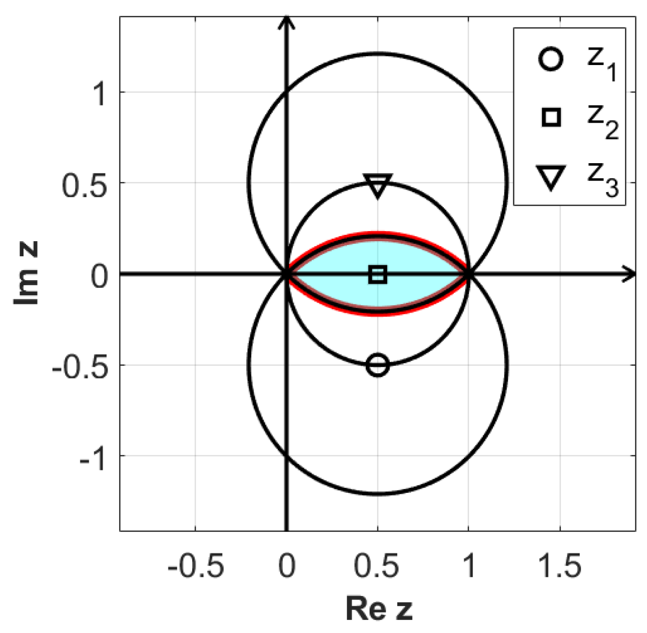
It is convenient to define the following points

$$\begin{array}{c}\hfill z_1=\frac{1}{2}-\frac{1}{2}i,z_2=\frac{1}{2},z_3=\frac{1}{2}+\frac{1}{2}i,\end{array}$$

(13)

representing the centres of the open disks

$$\begin{array}{c}\hfill D_1\left(z_1,\frac{\sqrt{2}}{2}\right),D_2\left(z_2,\frac{1}{2}\right),D_3\left(z_3,\frac{\sqrt{2}}{2}\right),\end{array}$$

(14)

and of the circles depicted in Figure 1

$$\begin{array}{c}\hfill C_1\left(z_1,\frac{\sqrt{2}}{2}\right),C_2\left(z_2,\frac{1}{2}\right),C_3\left(z_3,\frac{\sqrt{2}}{2}\right).\end{array}$$

(15)

Considering the real numbers $r_1,r_2,r_3,{\theta }_1,{\theta }_2,{\theta }_3$, by (4), (5), and (6), we obtain

$$\begin{array}{cc}\hfill u_1& =r_1{e}^{2\pi i{\theta }_1}=\sqrt{2}\left(\alpha -z_1\right)e^{-\frac{\pi i}{4}},\hfill \\ \hfill u_2& =r_2{e}^{2\pi i{\theta }_2}=2\left(\alpha -z_2\right),\hfill \\ \hfill u_3& =r_3{e}^{2\pi i{\theta }_3}=\sqrt{2}\left(\alpha -z_3\right)e^{\frac{\pi i}{4}}.\hfill \end{array}$$

(16)

By (16), we deduce that for a given $j=1,2,3$, if $\alpha \in D_j$, then we have $r_j<1$. Moreover, if $\alpha \in C_j$, then it follows that $r_j=1$. The distinct behaviours below emerge:

• If $\alpha \in D_1\cap D_2\cap D_3$, then $0<r_1,r_2,r_3<1$.
  One can easily check the set inclusion $D_1\cap D_3\subseteq D_2$.
• If $\alpha$ is in the interior of the complement of $D_1\cap D_3$, then $\max \{r_1,r_3\}>1$.
• If $\alpha \in C_1\cap C_2\cap C_3$, then $\alpha \in \{0,1\}$.

The boundary of the shaded region in Figure 1 consists of two arcs

$$U_1=C_1\cap D_3,U_3=C_3\cap D_1,$$

which can be parametrised as

$$\begin{array}{c}\hfill \alpha \left(t\right)=\left\{\begin{array}{cc}{z}_1+\frac{\sqrt{2}}{2}\left(\cos t+i\sin t\right),\hfill & t\in \left[\frac{\pi }{4},\frac{3\pi }{4}\right]\hfill \\ z_3+\frac{\sqrt{2}}{2}\left(\cos t+i\sin t\right),\hfill & t\in \left[\frac{5\pi }{4},\frac{7\pi }{4}\right].\hfill \end{array}\right.\end{array}$$

(17)

To describe the orbits of the sequences ${\left(a_n\right)}_{n\ge 0}$, ${\left(b_n\right)}_{n\ge 0}$, ${\left(c_n\right)}_{n\ge 0}$, and ${\left(d_n\right)}_{n\ge 0}$, one first needs to understand the behaviour of the sequence ${\left(z^n\right)}_{n\ge 0}$, where $z\in \mathbb{C}$ (see, for example, Lemma 2.1 in [13], or Lemma 5.2 in [14]), which is shown in Figure 2.

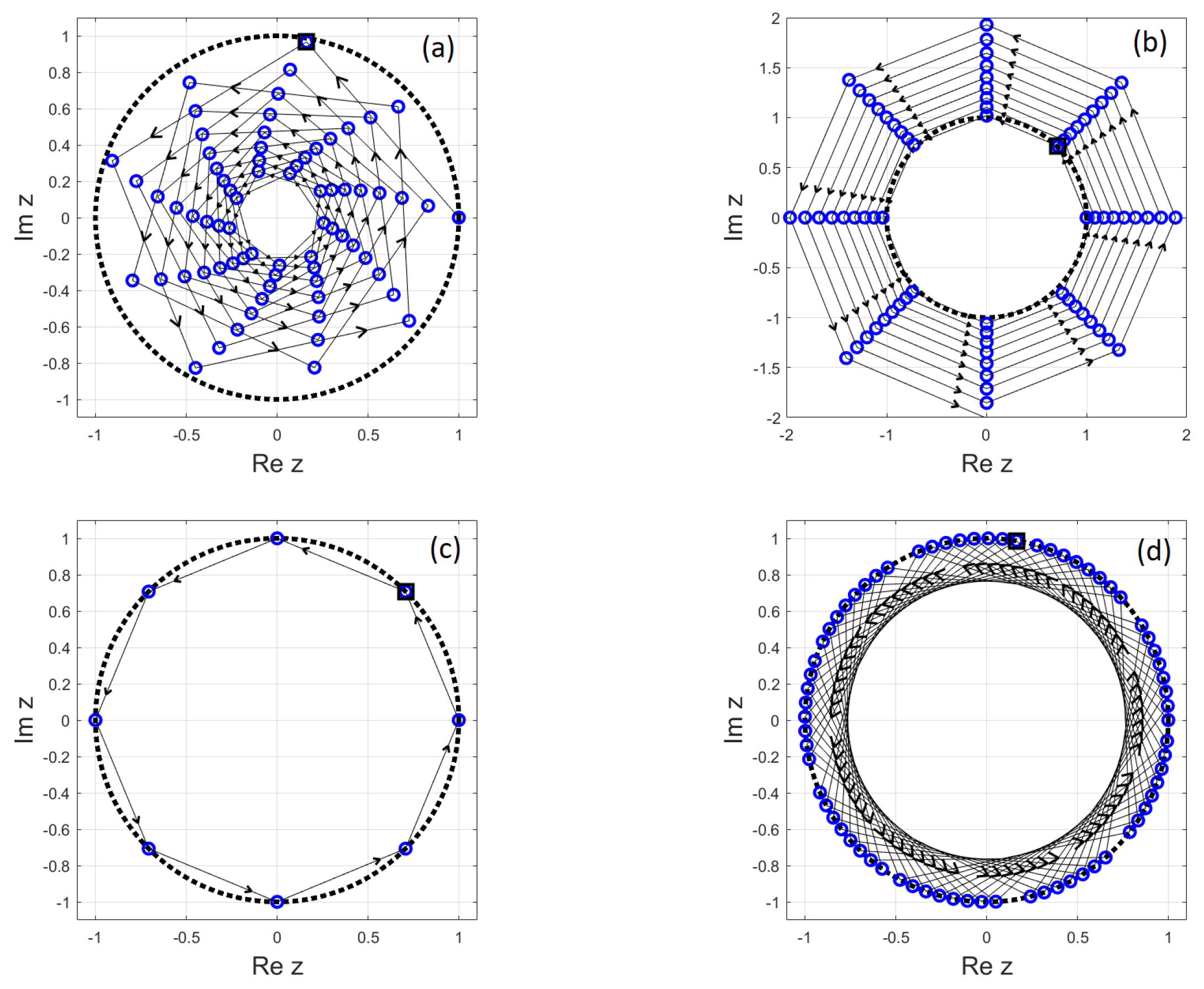
Lemma 1.

Let $z=r{e}^{2\pi i\theta }$, where $r\ge 0$, $\theta \in \mathbb{R}$. The orbit of ${\left(z^n\right)}_{n\ge 0}$ is:

$\left(a\right)$ A spiral convergent to 0 for $r<1$;

$\left(b\right)$ A divergent spiral for $r>1$;

$\left(c\right)$ A regular $k-$gon if z is a primitive $k-$th root of unity, $k\ge 3$;

$\left(d\right)$ A dense subset of the unit circle if $r=1$ and $\theta \in \mathbb{R}\setminus \mathbb{Q}$.

When $\theta =j/k\in \mathbb{Q}$ is irreducible, then the terms of the spirals obtained in (a) and (b) align along k rays.

To prove part (d), we use that $z^n=e^{2\pi in\theta }=e^{2\pi i(n\theta +m)}$ for $n\ge 0$ and m integers. By Kronecker’s Lemma ([15], Theorem 442), the set $\{n\theta +m:m,n\in \mathbb{Z},n\ge 0\}$ is dense in the set of real numbers $\mathbb{R}$; hence, the set $\{z^n:n\ge 0\}$ is dense within the unit circle.

As linear combinations of ${\left(u_1^n\right)}_{n\ge 0}$, ${\left(u_2^n\right)}_{n\ge 0}$, and ${\left(u_3^n\right)}_{n\ge 0}$, the sequences ${\left(a_n\right)}_{n\ge 0}$, ${\left(b_n\right)}_{n\ge 0}$, ${\left(c_n\right)}_{n\ge 0}$, and ${\left(d_n\right)}_{n\ge 0}$, given by the explicit Formula (10) in the complex plane, exhibit the following behaviour.

Lemma 2.

The patterns produced by Formula (10) are summarized below:

1. 

Convergent if $0<r_1,r_2,r_3<1$;

2. 

Divergent if $\max \{r_1,r_3\}>1$;

3. 

Periodic if $r_1=r_3=1$ (that is, when $\alpha =0$ or $\alpha =1$);

4. 

There are two distinct patterns when $0<\min \{r_1,r_3\}<\max \{r_1,r_3\}=1$.

Denoting $\theta ={\theta }_1$ if $r_1=1$ or $\theta ={\theta }_3$ if $r_3=1$, then the orbit:

(a) 

Has k convergent subsequences if $\theta =\frac{j}{k}$ is an irreducible fraction;

(b) 

Is dense within a circle when θ is irrational.

The details of the geometric patterns obtained in each case are presented below.

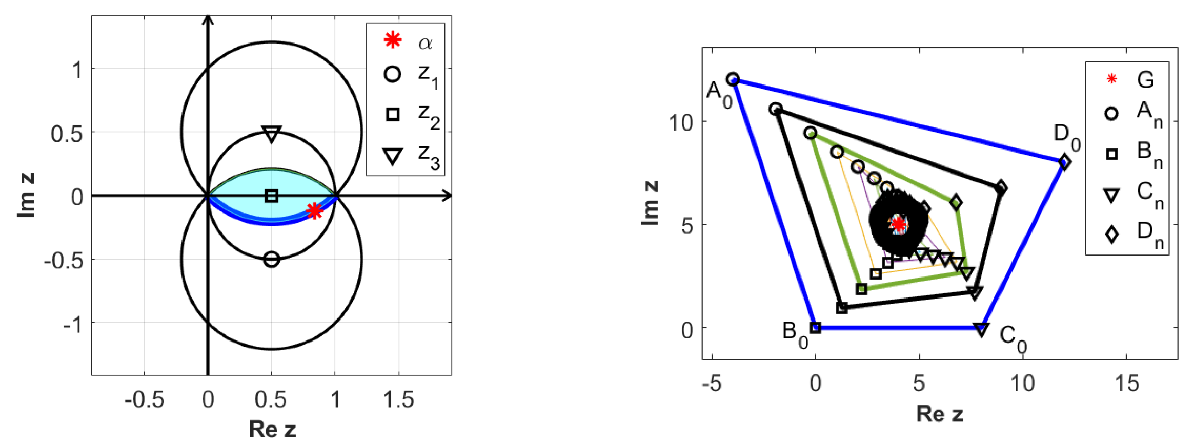
In all figures, we consider the initial polygon of complex coordinates

$$\begin{array}{c}\hfill A_0(-4+12i),B_0\left(0\right),C_0\left(8\right),D_0(12+1i),\end{array}$$

(18)

for which Formula (11) gives the values

$$\begin{array}{c}\hfill G=4+5i,M=-5+6i,N=-2+i,P=-1.\end{array}$$

(19)

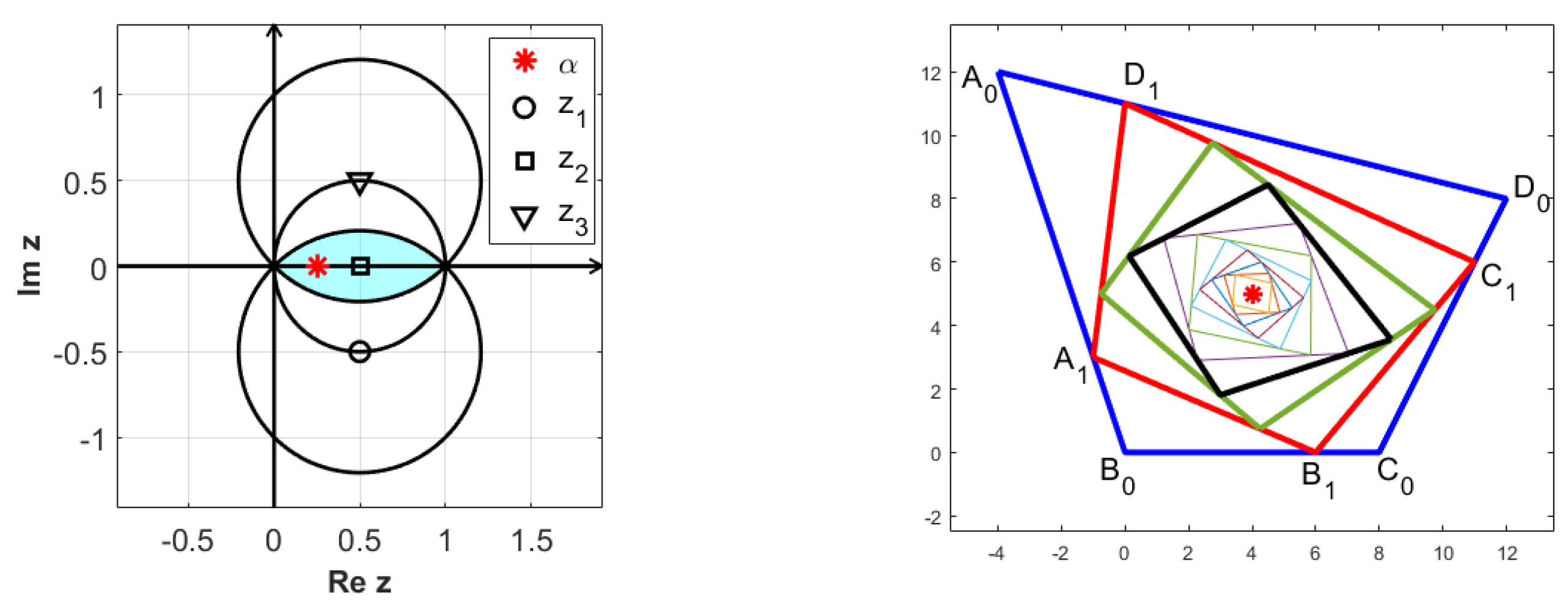
The position of $\alpha$ relative to relevant boundaries is indicated in the left diagram with a star, while the iterations of the polygon are displayed on the right, where the star indicates the position of the centroid. All the simulations have been implemented in Matlab^® 2021b.

4.1. Convergent Orbits

If $0<r_1,r_2,r_3<1$, then by (16), the sequences $u_1^n$, $u_2^n$, and $u_3^n$ are convergent if and only if $\alpha \in D_1\cap D_3$. Hence, by (10), we obtain that ${\left(a_n\right)}_{n\ge 0}$, ${\left(b_n\right)}_{n\ge 0}$, ${\left(c_n\right)}_{n\ge 0}$, and ${\left(d_n\right)}_{n\ge 0}$ converge to $g_0$. We can formulate the following result.

Theorem 1.

The following assertions hold:

(1)

The sequence ${\left(A_n{B}_n{C}_n{D}_n\right)}_{n\ge 0}$ is convergent if and only if $\alpha \in D_1\cap D_2$.

(2)

When the sequence ${\left(A_n{B}_n{C}_n{D}_n\right)}_{n\ge 0}$ is convergent, its limit is the degenerated quadrilateral at $G_0$, the centroid of the initial quadrilateral $A_0{B}_0{C}_0{D}_0$.

Proof. 

The intersection $D_1\cap D_3$ is shaded in Figure 1.

$\left(1\right)$ Clearly, $\alpha \in D_1\cap D_3$ is equivalent to $r_1<1$ and $r_3<1$ (in this case, one also has $\alpha \in D_2$). The relation (10) shows that the sequences ${\left(a_n\right)}_{n\ge 0}$, ${\left(b_n\right)}_{n\ge 0}$, ${\left(c_n\right)}_{n\ge 0}$, and ${\left(d_n\right)}_{n\ge 0}$ are convergent if and only if ${\left(u_1^n\right)}_{n\ge 0}$, ${\left(u_2^n\right)}_{n\ge 0}$, and ${\left(u_3^n\right)}_{n\ge 0}$ are convergent, which happens when $u_1^n\to 0$, $u_2^n\to 0$, and $u_3^n\to 0$.

$\left(2\right)$ Adding the equation in the system (1), one obtains that for every integer $n\ge 0$, we have $a_n+b_n+c_n+d_n=a_0+b_0+c_0+d_0=4g_0$, where $g_0$ is the complex coordinates of the centroid $G_0$ of the initial quadrilateral $A_0{B}_0{C}_0{D}_0$. Assume that $a_n\to a^{*}$, $b_n\to b^{*}$, $c_n\to c^{*}$, and $d_n\to d^{*}$. From system (1), we obtain

$$\left\{\begin{array}{c}{a}^{*}=\alpha a^{*}+(1-\alpha )b^{*}\hfill \\ b^{*}=\alpha b^{*}+(1-\alpha )c^{*}\hfill \\ c^{*}=\alpha c^{*}+(1-\alpha )d^{*}\hfill \\ d^{*}=\alpha d^{*}+(1-\alpha )a^{*}.\hfill \end{array}\right.$$

(20)

Because $\alpha \ne 1$, the only solution of this system is $a^{*}=b^{*}=c^{*}=d^{*}=g_0$. □

For $0<\alpha <1$, one has $\alpha \in D_1\cap D_3$, and moreover, in this case, the vertices $A_{n+1}$, $B_{n+1}$, $C_{n+1}$, $D_{n+1}$ are interior points of the segments $[A_n,B_n]$, $[B_n,C_n]$, $[C_n,D_n]$, and $[D_n,A_n]$, respectively. Such an example is depicted in Figure 3.

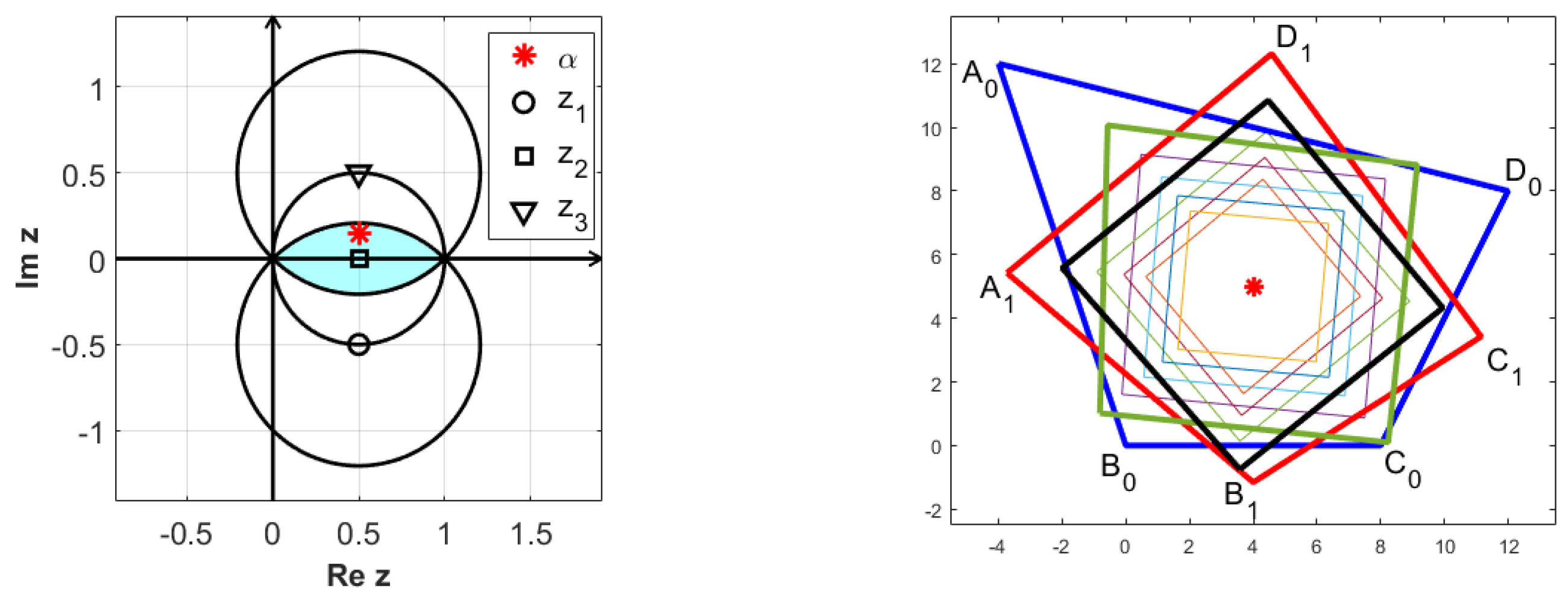
On the other hand, when the parameter $\alpha \in D_1\cap D_3$ is not real, the orbit is convergent, but the points are not aligned any more, as illustrated in Figure 4.

4.2. Periodic Orbits

If $r_1=r_2=r_3=1$, then $|\alpha -z_1|=|\alpha -z_3|=\frac{\sqrt{2}}{2}$ and $|\alpha -z_2|=\frac{1}{2}$, which can only happen for $\alpha \in C_1\cap C_2\cap C_3=\{0,1\}$.

Case 1. $\alpha =0$. From the system (1), for all $n\ge 0$, one obtains

$$a_{n+4}=b_{n+3}=c_{n+2}=d_{n+1}=a_n.$$

Similarly, $b_{n+4}=b_n$, $c_{n+4}=c_n$, and $d_{n+4}=d_n$, so the sequence terms satisfy

$$\left\{\begin{array}{c}{a}_n:a_0,b_0,c_0,d_0,a_0,b_0,c_0,\dots \hfill \\ b_n:b_0,c_0,d_0,a_0,b_0,c_0,d_0,\dots \hfill \\ c_n:c_0,d_0,a_0,b_0,c_0,d_0,a_0,\dots \hfill \\ d_n:d_0,a_0,b_0,c_0,d_0,a_0,b_0,\dots .\hfill \end{array}\right.$$

(21)

Case 2.$\alpha =1$. From the system (1), for all $n\ge 0$, one obtains

$$a_{n+1}=a_n,b_{n+1}=b_n,c_{n+1}=c_n,d_{n+1}=d_n,$$

so, in this case, the sequences are actually constant.

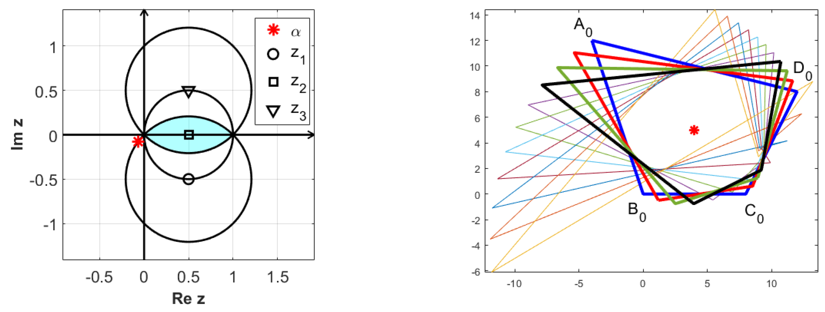
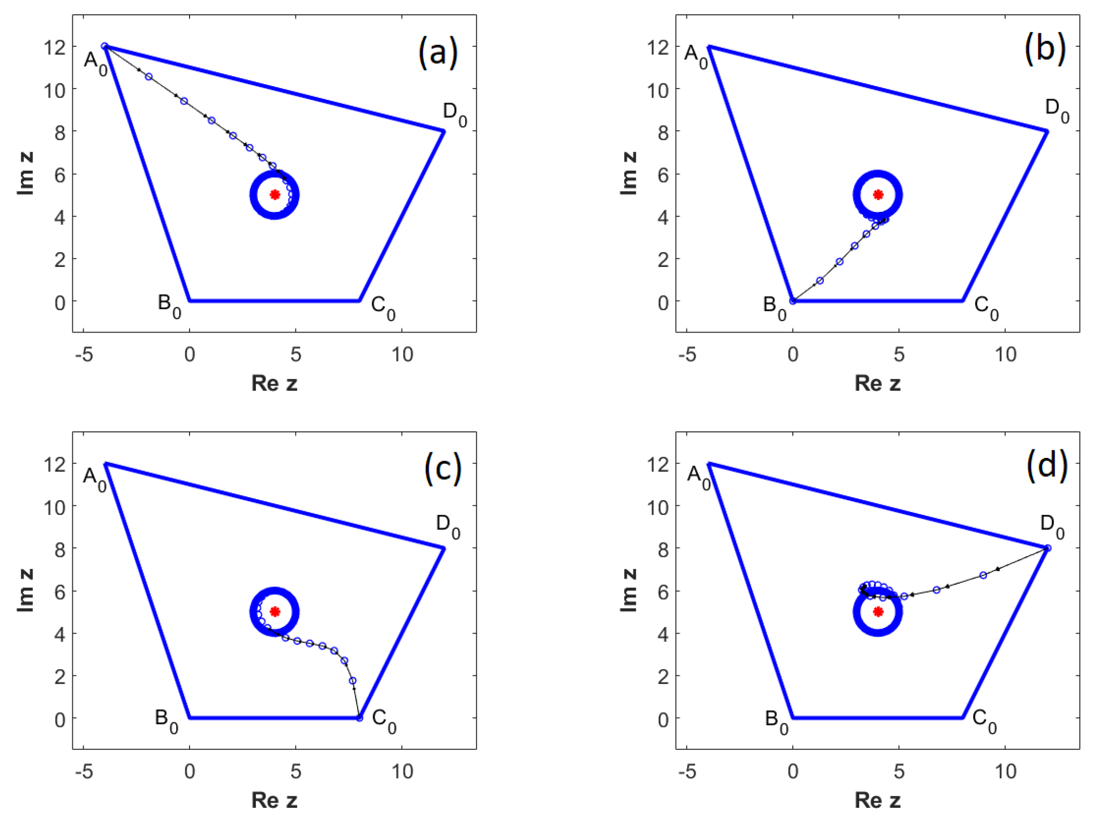
4.3. Divergent Orbits

If $\max \{r_1,r_3\}>1$, then $\alpha \in int\left[{\left(D_1\cap D_3\right)}^c\right]$; hence, by (16), either $u_1^n$ or $u_3^n$ are divergent. By Formula (10), the sequences ${\left(a_n\right)}_{n\ge 0}$, ${\left(b_n\right)}_{n\ge 0}$, ${\left(c_n\right)}_{n\ge 0}$, and ${\left(d_n\right)}_{n\ge 0}$ are divergent (as long as the corresponding coefficients M, N, P in (10) are not all vanishing).

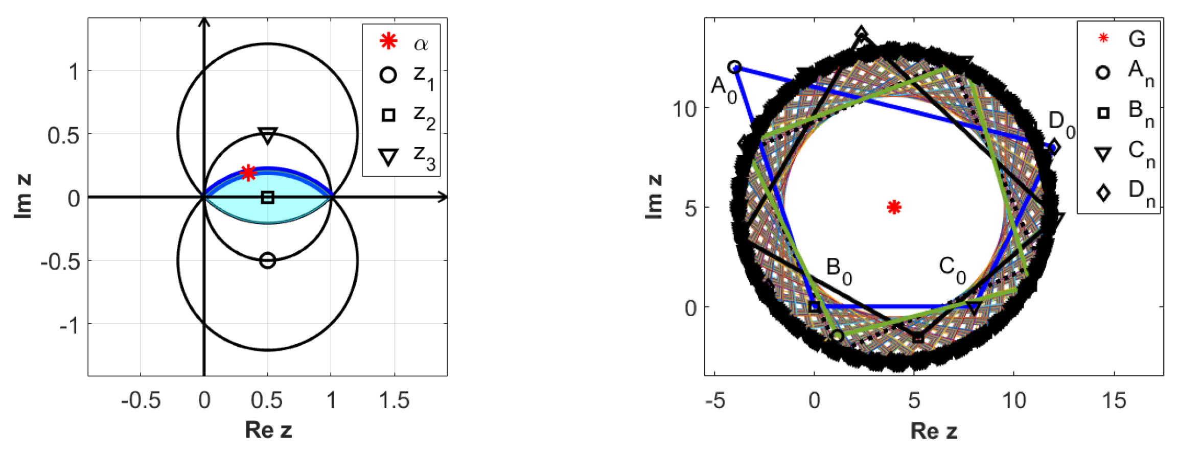
Figure 5 shows a divergent iteration. The diagram on the left we plot the position of $\alpha$, while on the right side we illustrate the polygons $A_n{B}_n{C}_n{D}_n$, $n=0,\dots ,10$.

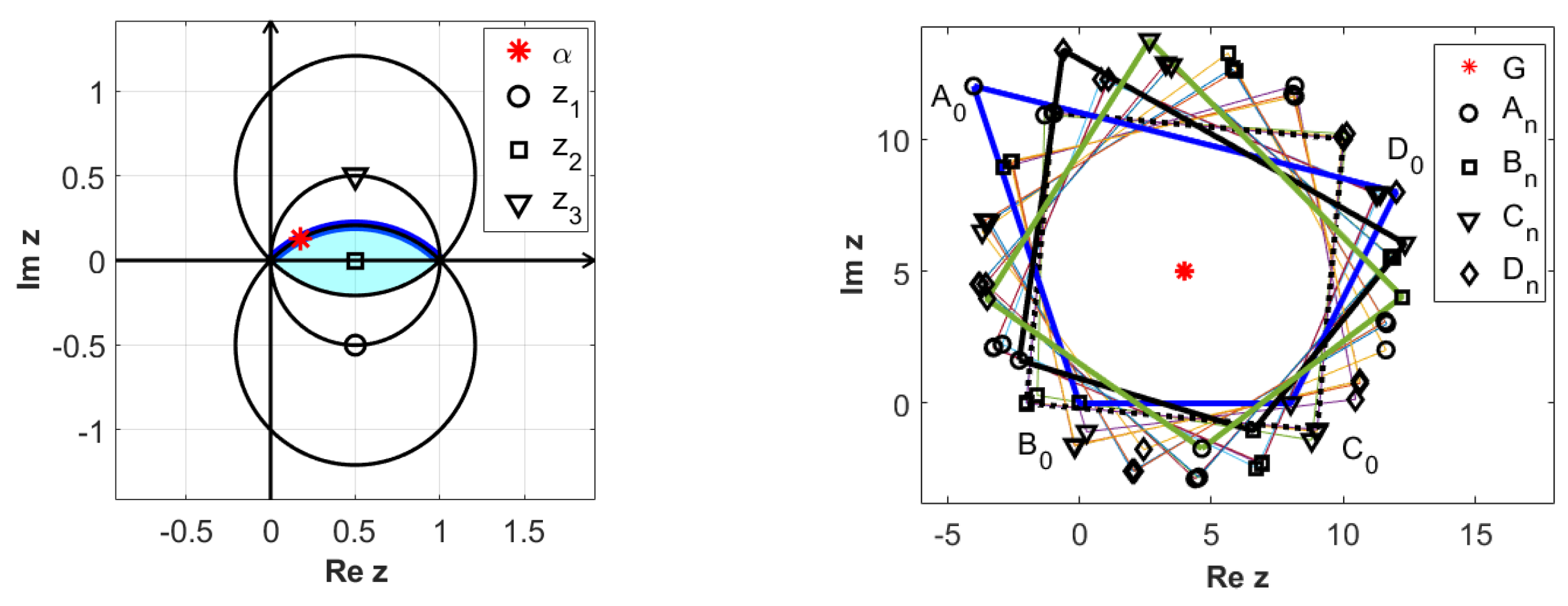
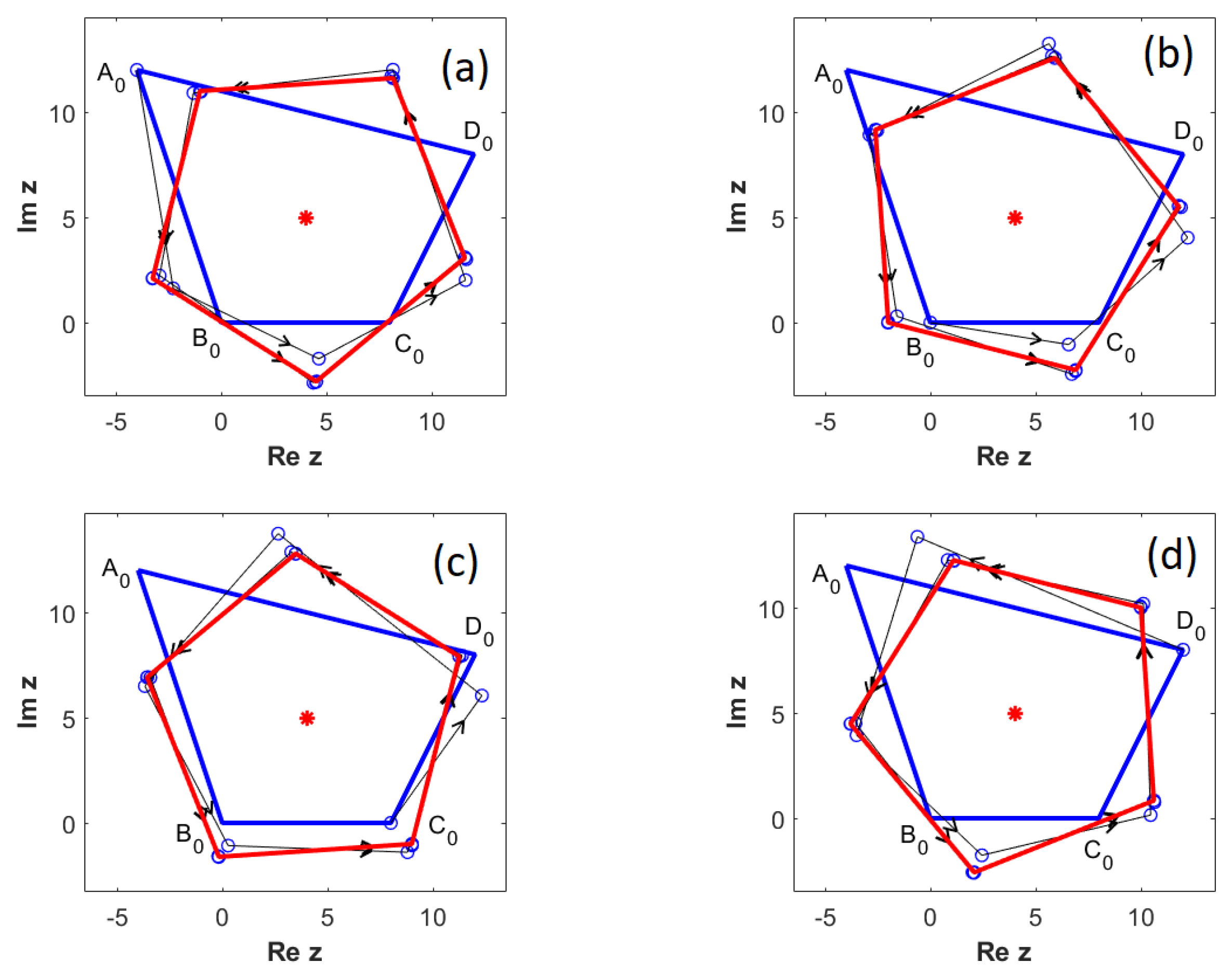
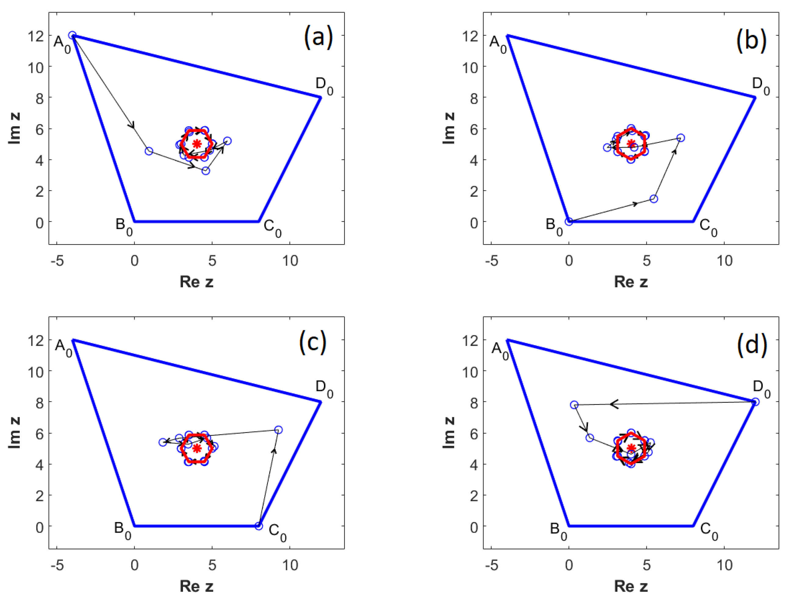
4.4. Orbits with a Finite Number of Convergent Subsequences

If $0<\min \{r_1,r_3\}<\max \{r_1,r_3\}=1$, then one either has $\alpha \in C_1\cap D_3$ for $r_1=1$, or $\alpha \in C_3\cap D_1$ for $r_3=1$. The orbit has a finite number of limit points if the complex argument $\theta$ of $u_1$ if $r_1=1$ or of $u_3$ if $r_3=1$ is rational.

4.4.1. Upper Arc of $C_1$

First, assume that $r_1=\max \{r_1,r_3\}=1$, i.e., $\alpha$ is on the upper arc $C_1\cap D_3$.

As $\alpha \in C_1$, there is $t\in \left[\frac{1}{8},\frac{3}{8}\right]$ with $\alpha =z_1+\frac{\sqrt{2}}{2}{e}^{2\pi it}$, so by (16), we obtain

$$\begin{array}{cc}\hfill u_1& =e^{2\pi i{\theta }_1}=\sqrt{2}\left(\alpha -z_1\right)e^{-\frac{\pi i}{4}}=e^{2\pi i\left(t-\frac{1}{8}\right)}.\hfill \end{array}$$

(22)

When ${\theta }_1=\frac{p}{q}$ is an irreducible fraction, the orbit has a finite number of convergent subsequences. Therefore, we have the following result.

Theorem 2.

If for the integers $0<p<q$, we have ${\theta }_1=\frac{p}{q}\in \left[0,\frac{1}{4}\right]$ is an irreducible fraction, then $u_1=e^{2\pi i\frac{p}{q}}$ and by Formula (10), the sequences ${\left(a_n\right)}_{n\ge 0}$, ${\left(b_n\right)}_{n\ge 0}$, ${\left(c_n\right)}_{n\ge 0}$, and ${\left(d_n\right)}_{n\ge 0}$ have subsequences which converge to the vertices of a regular $q-$gon centred at $G_0$ of radius $\left|M\right|$.

Proof. 

In this case, we have $u_1^{nq+j}=u_1^j$ for $j=0,\dots ,q-1$ and $u_2^n\to 0$ and $u_3^n\to 0$, so using the notations of (10) and (11), one obtains the relations

$$\begin{array}{cc}\hfill \underset{n\to \infty }{\lim }{a}_{nq+j}& =\underset{n\to \infty }{\lim }\left(g_0+M{u}_1^{nq+j}+N{u}_2^{nq+j}+P{u}_3^{nq+j}\right)=g_0+M{u}_1^j\hfill \\ \hfill \underset{n\to \infty }{\lim }{b}_{nq+j}& =\underset{n\to \infty }{\lim }\left(g_0+\left(Mi\right)u_1^{nq+j}+(-N)u_2^{nq+j}+(-Pi)u_3^{nq+j}\right)=g_0+\left(Mi\right)u_1^j\hfill \\ \hfill \underset{n\to \infty }{\lim }{c}_{nq+j}& =\underset{n\to \infty }{\lim }\left(g_0+(-M)u_1^{nq+j}+N{u}_2^{nq+j}+(-P)u_2^{nq+j}\right)=g_0+(-M)u_1^j\hfill \\ \hfill \underset{n\to \infty }{\lim }{d}_{nq+j}& =\underset{n\to \infty }{\lim }\left(g_0+(-Mi)u_1^{nq+j}+(-N)u_2^{nq+j}+\left(Pi\right)u_3^{nq+j}\right)=g_0+(-Mi)u_1^j,\hfill \end{array}$$

(23)

which ends the proof. This case is depicted in Figure 6. The sequences ${\left(a_n\right)}_{n\ge 0}$, ${\left(b_n\right)}_{n\ge 0}$, ${\left(c_n\right)}_{n\ge 0}$, and ${\left(d_n\right)}_{n\ge 0}$ are plotted in Figure 7. Moreover, one can check that for ${\theta }_1=1/5$ the limit polygon is a pentagon centred at $G_0$, of radius $\left|M\right|\simeq 7.81$ (by (19)). □

4.4.2. Lower Arc of $C_3$

Similarly, if $r_3=\max \{r_1,r_3\}=1$, then $\alpha$ is on the arc $C_3\cap D_1$ defined by (17). Therefore, there is $t\in \left[\frac{5\pi }{8},\frac{7\pi }{8}\right]$ with $\alpha =z_3+\frac{\sqrt{2}}{2}{e}^{2\pi it}$, and by (16), we obtain

$$\begin{array}{cc}\hfill u_3& =e^{2\pi i{\theta }_3}=\sqrt{2}\left(\alpha -z_3\right)e^{\frac{\pi i}{4}}=e^{2\pi i\left(t+\frac{1}{8}\right)}.\hfill \end{array}$$

(24)

The following result can be proved similarly to Theorem 2.

Theorem 3.

If for the integers $0<p<q$, we have ${\theta }_3=\frac{p}{q}\in \left[\frac{3}{4},1\right]$ is an irreducible fraction, then $u_1=e^{2\pi i\frac{p}{q}}$ and by Formula (10), the sequences ${\left(a_n\right)}_{n\ge 0}$, ${\left(b_n\right)}_{n\ge 0}$, ${\left(c_n\right)}_{n\ge 0}$, and ${\left(d_n\right)}_{n\ge 0}$ have q subsequences convergent to the vertices of four regular $q-$gons centred at $G_0$ of radius $\left|P\right|$.

The first 200 iterations obtained when ${\theta }_3=\frac{5}{6}$ are presented in Figure 8.

The sequences ${\left(a_n\right)}_{n\ge 0}$, ${\left(b_n\right)}_{n\ge 0}$, ${\left(c_n\right)}_{n\ge 0}$, and ${\left(d_n\right)}_{n\ge 0}$ are plotted in Figure 9. Similarly to (23), the limit polygon is a hexagon centred at G, which has radius $\left|P\right|=1$.

4.5. Dense Orbits

When $0<\min \{r_1,r_3\}<\max \{r_1,r_3\}=1$ but ${\theta }_1$ or ${\theta }_3$ are irrational modulo $2\pi$, the orbits of ${\left(a_n\right)}_{n\ge 0}$, ${\left(b_n\right)}_{n\ge 0}$, ${\left(c_n\right)}_{n\ge 0}$, and ${\left(d_n\right)}_{n\ge 0}$ are dense within circles.

4.5.1. Upper Arc of $C_1$

First, assume that $0<r_3<r_1=1$, i.e., $\alpha$ is on the upper arc $C_1\cap D_3$. Using the notations in (22), the following result can be deduced from Lemma 1 (d).

Theorem 4.

If $r_1=1$ and ${\theta }_1\in \left[0,\frac{1}{4}\right]$ is irrational, then the set of limit points for each of the sequences ${\left(a_n\right)}_{n\ge 0}$, ${\left(b_n\right)}_{n\ge 0}$, ${\left(c_n\right)}_{n\ge 0}$, and ${\left(d_n\right)}_{n\ge 0}$ is the circle centred at $G_0$ of radius $\left|M\right|$.

Proof. 

By (10), we have $a_n=g_0+M{u}_1^n+N{u}_2^n+P{u}_3^n$, with M, N, and P constants given by (11). Because $|u_2|<1$, $|u_3|<1$, we have $a_n=g_0+M{u}_1^n+z_n$, where ${\lim }_{n\to \infty }{z}_n=0$.

Let z be an arbitrary point on the circle of centre $G_0$ and radius $\left|M\right|$. If $M=0$, then ${\lim }_{n\to \infty }{a}_n=g_0$. Otherwise, denoting $z^{\prime }=\frac{z-g_0}{M}$, we have $z^{\prime }\in \mathcal{C}(0,1)$. Because $u_1=e^{2\pi i{\theta }_1}$ with ${\theta }_1$ irrational, by Lemma (1), it follows that there is a subsequence $n_1<n_2<\cdots$ such that ${\lim }_{k\to \infty }{u}_1^{n_k}=z^{\prime }$. For $\epsilon >0$, one can find $K_1\left(\epsilon \right)$ and $K_2\left(\epsilon \right)$ such that

$$\begin{array}{c}\hfill |u_1^{n_k}-z^{\prime }|<\frac{1}{\left|M\right|+1}\epsilon ,k\ge K_1\left(\epsilon \right)\mathrm{and}\left|z_{n_k}\right|<\frac{1}{\left|M\right|+1}\epsilon ,k\ge K_2\left(\epsilon \right),\end{array}$$

hence, for $k\ge \max \{K_1\left(\epsilon \right),K_1\left(\epsilon \right)\}$, one obtains

$$\begin{array}{c}\hfill |a_{n_k}-z|=|g_0+M{u}_1^{n_k}+z_{n_k}-g_0-M{z}^{\prime }|\le |M|·|u_1^{n_k}-z^{\prime }|+|z_{n_k}|<\epsilon ,\end{array}$$

hence ${\lim }_{k\to \infty }{a}_{n_k}=z$. This shows that z is a limit point for the sequence ${\left(a_n\right)}_{n\ge 0}$. Analogously, this is proved for ${\left(b_n\right)}_{n\ge 0}$, ${\left(c_n\right)}_{n\ge 0}$ and ${\left(d_n\right)}_{n\ge 0}$. □

Figure 10 illustrates the position of $\alpha$ and the polygons obtained for $n=10$ iterations, respectively, when $\alpha \in C_1\cap D_3$. Figure 11 depicts the vertices of the original quadrilateral of affixes ${\left(a_n\right)}_{n\ge 0}$, ${\left(b_n\right)}_{n\ge 0}$, ${\left(c_n\right)}_{n\ge 0}$, and ${\left(d_n\right)}_{n\ge 0}$, and 200 iterations.

4.5.2. Lower Arc of $C_3$

When $0<r_1<r_3=1$, $\alpha$ is on the arc $C_3\cap D_1$ defined by (17), as in Figure 12. Using the notations in (24), we can formulate the following result.

Theorem 5.

If $r_3=1$ and ${\theta }_3\in \left[\frac{3}{4},1\right]$ is irrational, then the set of limit points for each of the sequences ${\left(a_n\right)}_{n\ge 0}$, ${\left(b_n\right)}_{n\ge 0}$, ${\left(c_n\right)}_{n\ge 0}$, and ${\left(d_n\right)}_{n\ge 0}$ is the circle centred at $G_0$ of radius $\left|P\right|$.

Proof. 

The proof follows the similar lines as for Theorem 4, but now by (10), one has $a_n=g_0+M{u}_1^n+N{u}_2^n+P{u}_3^n$. Because $|u_1|<1$, $|u_2|<1$, we obtain $a_n=g_0+z_n+P{u}_3^n$, where ${\lim }_{n\to \infty }{z}_n=0$. Figure 12 shows the position of $\alpha$ and the first $n=10$ iterations, respectively, when $\alpha \in C_3\cap D_1$. Figure 13 plots the vertices of the original quadrilateral of affixes ${\left(a_n\right)}_{n\ge 0}$, ${\left(b_n\right)}_{n\ge 0}$, ${\left(c_n\right)}_{n\ge 0}$, and ${\left(d_n\right)}_{n\ge 0}$, and 200 iterations. □