A New Fuzzy Robust Control for Linear Parameter-Varying Systems

Abstract

The linear parameter-varying (LPV) models have broad applications in advanced mathematics and modern control systems. This paper introduces a new method for controlling the LPV systems. This method includes the gain-scheduled state-feedback technique and a fuzzy system to calculate the state-feedback gain. The main goal of the control system is to stabilize the system and bring its states to equilibrium points. Linear matrix inequalities calculate feedback gains to stabilize the system. On the other hand, a fuzzy control system also produces a combined signal with the primary controller signal to speed up this operation. Lyapunov’s theory is used to guarantee the control system’s stability. Finally, to evaluate the performance of the proposed control system, the inverted pendulum has been investigated as a case study. The results show that the proposed method has good efficiency and performance.

1. Introduction

The behavior of many dynamic systems can be analyzed with a high accuracy by linear parameter-varying (LPV) models. These models have attracted a lot of attention. One of the main reasons for such attention is the potential application of LPV models in advanced mathematical tools, such as linear matrix inequalities (LMIs), the concept of convex systems, and interest-scheduling controllers [1,2].

The methods that are frequently used for this problem include optimization-based techniques (conditions according to an algorithm minimum/maximum), Richard equations, and convex programming [3]. Most of the methods presented in these articles use unequal algorithms and the linear matrices of the iteration. The basic form of approach repetition is that there is no systematic theory to stop the repetition and reach value without a final value. In operational applications, the objective function after low repetitions achieves this. However, the values obtained are not necessarily the general response. In other words, the presented methods have no guarantee of convergence, and there is no specific response. Another drawback is the lack of a general rule for giving the initial value to recurring parameters. Thus, conservatism is an integral part of repetitive algorithms [4,5].

In the absence of economic restrictions and physical conditions, such as the location of sensors, the state-feedback method can also be used. In some applications, operational sensitivities and control attitudes require feedback directly from a particular situation. For example, in many interceptors, the roll rate of a typical missile is essential. Therefore, sometimes the roll rate of a typical missile must be measured directly. Most articles’ common assumption is that accurate scheduling parameter values are available in real time. This is a limiting condition in operational applications because the presence of measuring noises, calibration errors, and other uncertainties is inevitable. Therefore, the designed controllers must resist the uncertainties created by the scheduling parameters [6,7]. Moreover, in many operational applications, only some physical parameters can be measured, and others lack parametric certainties. As a result, parametric uncertainties can also lead to indefinite scheduling parameters. In [8,9], the effect of the inaccuracy of scheduling parameters has been investigated. Only aggregate indeterminate is assumed to be present. Inaccurate scheduling parameters in the form of ${\tilde{\theta }}_i\left(t\right)={\theta }_i\left(t\right)+{\delta }_i\left(t\right)$ have been represented.

Finally, using the mentioned scheduling parameters, the dynamic output of the state-feedback controller is designed. A similar display for incorrect scheduling parameters is provided in [10]. In this reference, the design is based on the dynamic output of the state-feedback controller. In [11], the problem of designing a full-order state-feedback controller in incorrect scheduling parameters is considered. The main disadvantage of this study is that the bias errors are not considered. In other words, the inaccurate scheduling parameter is considered as $\widehat{\theta }\left(t\right)=\lambda \theta \left(t\right)$, in which $\theta \left(t\right)$, $\widehat{\theta }\left(t\right)$, and $\lambda$ are the exact scheduling parameters, inaccurate scheduling parameters, and fixed numbers, respectively. In [12], the full-order state-feedback controller in the presence of incorrect scheduling parameters has been designed. In this design, two types of collapsible and proportional uncertainties have been investigated. In [13], the inaccurate parameters in the form of ${\tilde{\theta }}_i\left(t\right)=\left(1+{\delta }_i^p\left(t\right)\right)\left({\theta }_i\left(t\right)+{\delta }_i^a\left(t\right)\right)$ are considered and the full-order state-feedback controller is designed. ${\delta }_i^a\left(t\right)$ and ${\delta }_i^p\left(t\right)$ can be interpreted as additional and proportional uncertainties. Moreover, in [10], the effects of inaccurate scheduling parameters in the design of state-feedback controllers have been investigated. The inequalities obtained in this work are solved by the iterative method. As mentioned earlier, iterative approaches face many challenges, including setting initial conditions [14].

The studies mentioned above use multiplicative and collapsible models to express inaccurate scheduling parameters and design processes. One of the most critical challenges in gain-scheduled controllers is the presence of time-invariant uncertainty in the LPV systems. Because of gain scheduling, controllers make sense of time changes. However, the mentioned uncertainties are fixed and uncertain. Indeed, we are dealing with two opposing concepts. Therefore, the interest rate controller designer’s main challenge is to consider both concepts. In such a case, the difficulty of design increases when uncertainty that does not change with time cannot be explicitly extracted. Few articles have studied both of these phenomena. It should be noted that the studies above have considered parametric uncertainties without using the parameter variable systems approach [15,16].

Although the approaches presented in these articles have been practical, the undeniable problem of the proposed approaches in the mentioned articles is their presence of computational difficulties, such as complex return relations, and the imposition of the assumptions on the dynamics of nonlinear systems. For these reasons, designers prefer to use the parameter variable systems approach to control nonlinear systems. Researchers have used parametric variable systems in [17] and considered parametric uncertainties that do not change with time. The reference [18] presents the feedback-mode control method in the presence of parametric uncertainties that do not change with time. One of the main challenges of this paper is to consider the input matrix constant. In other words, only the state matrix is considered a variable parameter. In this paper, the input matrix is affected by parametric uncertainties that do not change over time. However, it is assumed that the range of these uncertainties is small, and as a result, these uncertainties have been replaced by their own mean values. This causes the input matrix to be considered constant. It is quite clear that if such a limiting assumption is taken into account, the possibility of system instability in operating conditions will be greatly increased. Similar issues have been investigated in [19,20,21]. The adjustment of the feedback gain has been investigated in various studies [22]. Various methods, such as fuzzy [23] and adaptive [24], have been proposed to achieve this goal. In [25], a feedback gain adjustment method for a quadcopter with three degrees of freedom is proposed.

System state-space matrices are considered uncertain due to invariant parametric uncertainties. The most critical challenge of this effect is the constraint imposed on the system state-space matrices. In other words, the assumption was that the uncertainties in the system state-space matrices could be explicitly extracted from the mentioned matrices. More precisely, it is assumed that each of the indeterminate matrices of the system state space can be rewritten as two separate components, the first containing only time-invariant parametric uncertainties and the second containing exact timing parameters. However, it is impossible to separate unchanging parametric uncertainties over time in many applications. For example, aerodynamic coefficients can be considered parametric uncertainties that do not change over time in interceptor systems. However, the dynamic equations governing the interceptor are so complex that these coefficients cannot be extracted purely. This is true in many complex operational applications. To overcome this problem, the reference [26] of the feedback law has proposed a robust state resistant to parametric uncertainties with time. In the mentioned reference, the auxiliary timing parameters of the upper and lower boundaries of the variable with time have been used. These parameters are obtained by maximizing and minimizing the indefinite timing parameters at any given time and in the entire interval provided for the indefinite. Such a process must be online and impose a sizeable computational volume on the processor. For this reason, this method has limitations in practical applications.

The present paper discusses the design of feedback controllers for the robust state timing of variable parametric linear systems in the presence of time-invariant parametric uncertainties. In the first step, we select the desired values from the intervals provided for the mentioned uncertainties and place them in the indefinite timing parameters instead of the existing uncertainties. As a result, we will have specific timing parameters. Therefore, the variable system with the parameter is known. However, the specified parameters cannot be used to create the final controller because the selected values for the uncertainties are not necessarily equal to the correct values. Therefore, we are looking for a way to compensate for this difference. In these cases, we will use the proposed new non-binding parameters. Thus, according to the intervals defined for parametric uncertainties and the intervals of changes in parameter-variable system modes, we find values of the parametric uncertainties that minimize and maximize the indeterminate timing parameters. New timing parameters will be obtained by placing the ready-made values in the indefinite timing parameters and their combinations. The feedback controller is then proposed in a state that the new parameters have timed. The proposed controller is resistant to all values of the given intervals for parametric uncertainties. In other words, the closed-loop system will remain stable with whatever arbitrary value we choose for the mentioned uncertainties. The proposed controller contains all the information about the minimum and maximum indefinite scheduling parameters. The concept of system convexity, the matrix linear inequalities, and the Lyapunov stability concept are the tools used to find the ultimate controller. Finally, the proposed law controls the rolling channel of a kind of air-to-ground interceptor. The results obtained in the simulations are compared with those of the hardware laboratory in the loop. One of the solutions to control theory problems, such as optimization, changes in system dynamics, changes in parameters, etc., is using computational intelligence. For example, neural networks, fuzzy systems, and evolutionary algorithms can be used as a complement to classical control methods.

The combination of fuzzy systems and neural networks is now used in various applications [27]. Currently, various methods of controlling technological objects in a fuzzy environment based on mathematical models have been presented. These methods can work well to deal with uncertainties [28,29]. In [30], an adaptive neuro-fuzzy sliding mode control method is proposed. The proposed method in this study has been implemented on an autonomous underwater vehicle (AUV) and the uncertain behavior of the system has been resolved by a neural network. Another problem that this study has solved is the chattering phenomenon. This problem is solved using an adaptive fuzzy proportional–integral control. The fractional orders of the controller of the previous study, i.e., the adaptive neuro-fuzzy sliding mode control in [31], have been used for the class of fuzzy singularly perturbed systems. This method works well to deal with system uncertainties. Dealing with internal disturbances is one of the challenges of any system. In summary, the innovations presented in this article are:

• Present a novel robust gain-scheduled control for LPV systems.
• A fuzzy control system design for the online determination of feedback gain.
• Proof of control system stability based on the Lyapunov theory.

In the remaining parts, some preliminaries are given in Section 2. The problem is described in Section 3. Then, a robust state-feedback controller is designed in Section 4. The simulation results obtained using the proposed controller are given in Section 5. Finally, the discussion and conclusions are presented in Section 6 and Section 7, respectively.

2. Preliminaries

In the following, the symbols used in this article are presented. I is a single matrix with suitable dimensions. ${\left[C_i\right]}_p$, ${\left[C_{\left(i,j\right)}\right]}_{p\times p}$, $\Theta \left(t,\eta \right){\left|\right.}_{\eta ={\eta }_c}$, and $\Theta \left(t,{\eta }_{New}\right){\left|\right.}_{\eta ={\eta }_{New}}$ are defined as follows:

$${\left[C_i\right]}_p=\left[C_1{C}_2\dots C_p\right]$$

(1)

$${\left[C_{\left(i,j\right)}\right]}_{p\times p}=\left[\begin{array}{ccc}\begin{array}{cc}{C}_{\left(1,1\right)}& C_{\left(1,2\right)}\end{array}& \dots & C_{\left(1,p\right)}\\ \begin{array}{cc}{C}_{\left(2,1\right)}& C_{\left(2,2\right)}\end{array}& \dots & C_{\left(2,p\right)}\\ \begin{array}{c}\begin{array}{cc}⋮& ⋮\end{array}\\ \begin{array}{cc}{C}_{\left(p,1\right)}& C_{\left(p,2\right)}\end{array}\end{array}& \begin{array}{c}\ddots \\ \dots \end{array}& \begin{array}{c}⋮\\ C_{\left(p,p\right)}\end{array}\end{array}\right]$$

(2)

$$\Theta \left(t,\eta \right){\left|\right.}_{\eta ={\eta }_c}=\left\{{\theta }_i\left(t,\eta \right){\left|\right.}_{\eta ={\eta }_c}\left|i=1,2,\dots ,p\right.\right\}$$

(3)

$$\Theta \left(t,{\eta }_{New}\right){\left|\right.}_{\eta ={\eta }_{New}}=\left\{{\theta }_{iNew}\left(t,{\eta }_{New}\right){\left|\right.}_{\eta ={\eta }_{New}}\left|i=1,2,\dots ,p\right.\right\}$$

(4)

where $\Theta \left(t,\eta \right)\in R^p$, $\Theta \left(t,{\eta }_{New}\right){\left|\right.}_{\eta ={\eta }_{New}}\in R^p$ are the set of specific and new vector scheduling parameters, respectively, $\eta$ is a vector of parametric uncertainties that does not change with time in indefinite scheduling parameters, ${\eta }_c$ is the vector of arbitrary values selected from the defined range for parametric uncertainties, which by placing them in indefinite scheduling parameters, specific scheduling parameters will be obtained. The vector ${\eta }_{New}$ contains ${\eta }_{i,min},{\eta }_{i,max}$ ($i=1,2,3,\dots ,p$) which are values of parametric uncertainties that make the $-i$ of the indefinite timing parameter the minimum and maximum, respectively. The symbol (*) represents the elements below the original diameter of a symmetric matrix. Moreover, in this paper, parametric uncertainties do not change with time. Parameters $p\left(t\right),\rho \left(t\right),I_x,h,V\left(t\right),S,D,C_{L_{\delta a}},{\delta }_a\left(t\right)$, and $C_{L_p}$, respectively, denote rolling rate (deg/sec), air intake (kg/m${}^3$), moment of inertia around the longitudinal axis (kg-m${}^2$), height (m), interceptor velocity (m/s), interceptor base area (m${}^2$), the diameter of the interceptor (m), the coefficient of change of its rolling torque due to changes in its rolling control (deg${}^{-1}$), its rolling command (deg), and the damping coefficient of its rolling channel (deg${}^{-1}$). Moreover, $M\left(t\right)$ is the velocity in Mach.

3. Problem Description

Consider a variable system with the following indeterminate parameter:

$$\dot{X}\left(t\right)=A\left(\Theta \left(t,\eta \right)\right)X\left(t\right)+B\left(\Theta \left(t,\eta \right)\right)u\left(t\right)$$

(5)

where $A\left(\Theta \left(t,\eta \right)\right)\in R^{p\times p}$ and $B\left(\Theta \left(t,\eta \right)\right)\in R^{p\times m}$ are the state and input matrices and $\Theta \left(t,\eta \right)\in R^p$ are the vectors of the indeterminate timing, respectively. P is the number of corners. Moreover, $X\left(t\right)\in R^p$ and $u\left(t\right)\in R^m$ are mode vectors and control inputs, respectively. Select the desired value of the parametric uncertainties, ${\eta }_c$, from the defined intervals for the existing uncertainties and place it in $\Theta \left(t,\eta \right)\in R^p$. Then, we have a variable linear system with a specific parameter as follows:

$$\dot{X}\left(t\right)=A\left(\Theta \left(t,\eta \right)\left|{}_{\eta ={\eta }_c}\right.\right)X\left(t\right)+B\left(\Theta \left(t,\eta \right)\left|{}_{{\eta }_{={\eta }_c}}\right.\right)u\left(t\right)$$

(6)

which we call $\Theta \left(t,\eta \right)\left|{}_{\eta ={\eta }_c}\right.\in R^p$ as a vector of specified timing parameters. Moreover, the input and state matrices shown as convex are expressed in the following relation:

$$A\left(\Theta \left(t,\eta \right)\left|{}_{\eta ={\eta }_c}\right.\right)=\sum _{i=1}^p{A}_i{\theta }_i\left(t,\eta \right)\left|{}_{\eta ={\eta }_c}\right.$$

(7)

where

$$B\left(\Theta \left(t,\eta \right)\left|{}_{\eta ={\eta }_c}\right.\right)=\sum _{i=1}^p{B}_i{\theta }_i\left(t,\eta \right)\left|{}_{\eta ={\eta }_c}\right.$$

(8)

where $A_i$ and $B_i$ are convex polygonal angles. Suppose the state-feedback control rule is defined as follows:

$$u\left(t\right)=K\left({\Theta }_{New}\left(t,{\eta }_{New}\right)\right)X\left(t\right)=\sum _{i=1}^p\left(K_i{\theta }_{iNew}\left(t,{\eta }_{New}\right)\right)X\left(t\right)$$

(9)

where $i=1,2,\dots ,p$ and $K_i$ are fixed matrices that must be calculated. In traditional methods, this parameter is usually calculated by trial and error, but in this article, a fuzzy system is used to calculate and update the $K_i$. ${\Theta }_{New}\left(t,{\eta }_{New}\right)\in R^p$ is the vector of the new scheduling parameters and $K\left({\Theta }_{New}\left(t,{\eta }_{New}\right)\right)$ is the feedback mode of the scheduling mode. Moreover, the vector ${\eta }_{New}$ contains ${\eta }_{imin}$ and ${\eta }_{imax}$, where $i=1,2,\dots ,p$. The terms ${\eta }_{imin}$ and ${\eta }_{imax}$ denote the minimum and maximum values of parametric uncertainties.

By substituting Equation (9) in Equation (6), we will obtain the following equation:

$$\dot{X}\left(t\right)=A_c\left(\Theta \left(t,\eta \right)\left|{}_{\eta ={\eta }_c}\right.,{\Theta }_{New}\left(t,{\eta }_{New}\right)\right)X\left(t\right)$$

(10)

where

$$\begin{array}{c}{A}_c\left(\Theta \left(t,\eta \right)\left|{}_{\eta ={\eta }_c}\right.,{\Theta }_{New}\left(t,{\eta }_{New}\right)\right)=\hfill \\ A\left(\Theta \left(t,\eta \right)\left|{}_{\eta ={\eta }_c}\right.\right)+B\left(\Theta \left(t,\eta \right)\left|{}_{\eta ={\eta }_c}\right.\right)K\left({\Theta }_{New}\left(t,{\eta }_{New}\right)\right)\hfill \end{array}$$

(11)

Therefore, the design problem of the feedback control timing mode of variable linear systems with an indeterminate parameter is defined as follows. Consider a variable linear system with an indeterminate parameter, Equation (5). The aim is to find the K-state-feedback gain, so as to overcome the uncertainty of the parameter that does not change over time, and finally, the stable closed-loop system is asymptotic. New scheduling parameters must be defined in this path. In the next section, new scheduling parameters and robust mode feedback controller design methods are presented.

4. The Proposed Control System

As we have stated, by selecting the desired values from the defined range for parametric uncertainties and placing them in indefinite scheduling parameters, we achieve specific scheduling parameters. However, the selected values are not necessarily equal to the actual values. Therefore, new scheduling parameters must be introduced to ensure that the proposed interest rate scheduling controller creates a smooth and, ultimately, asymptotic stability of the loop system depending on all values associated with the parameter uncertainty intervals. Now, suppose that the specified timing parameters meet the relational constraints. The new scheduling parameters are then defined as follows:

$${\theta }_{iNew}\left(t,{\eta }_{New}\right)=\frac{a_i\left(t\right)}{b\left(t\right)}$$

(12)

where $a_i\left(t\right)$ and $b\left(t\right)$ are as follows:

$$\begin{array}{c}{\displaystyle a_i\left(t\right)=\left(p-1\right){\theta }_i\left(t,\eta \right)\left|{}_{\eta ={\eta }_{imin}}\right.+}\hfill \\ {\displaystyle \left(p-1\right)\left({\theta }_i\left(t,\eta \right)\left|{}_{\eta ={\eta }_{imax}}\right.+\mu \right)-\sum _{\begin{array}{c}j=1\\ j\ne i\end{array}}^p({\theta }_i\left(t,\eta \right)\left|{}_{\eta ={\eta }_{jmax}}\right.-\mu )+}\hfill \\ {\displaystyle \frac{1}{p-1}\sum _{\begin{array}{c}j=1\\ j\ne i\end{array}}^p\sum _{\begin{array}{c}\ell =1\\ \ell \ne j\end{array}}^p\left({\theta }_j\left(t,\eta \right)\left|{}_{\eta ={\eta }_{\ell max}}\right.\right)+{\theta }_i\left(t,\eta \right)\left|{}_{\eta ={\eta }_c}\right.}\hfill \end{array}$$

(13)

$${\displaystyle b\left(t\right)=\left(p-1\right)\left(\sum _{q=1}^p{\theta }_q\left(t,\eta \right)\left|{}_{\eta ={\eta }_{qmax}}\right.+\sum _{q=1}^p{\theta }_q\left(t,\eta \right)\left|{}_{\eta =min}\right.+\sum _{q=1}^{p}2\mu +\frac{1}{p-1}\right)}$$

(14)

So that $i=1,2,\dots ,p$ and ${\eta }_{imin}$ and ${\eta }_{imax}$ are resistances of parametric uncertainties that make the parameter $-i$ indefinite, minimum and maximum, respectively. Parameter $\mu$ is a non-negative constant value that establishes the inequality $\left({\theta }_i\left(t,\eta \right)\left|{}_{\eta ={\eta }_{imax}}\right.+\mu \right)\ge \left({\theta }_i\left(t,\eta \right)\left|{}_{\eta ={\eta }_{jmax}}\right.-\mu \right)$ for $i\ne j$ and $i=1,2,\dots ,p$. Parameter $\eta$ is a parametric uncertainty that does not change over time. ${\eta }_{cis}$ is the preferred vector of choice. Parameter ${\theta }_i\left(t,\eta \right)\left|{}_{\eta ={\eta }_{imin}}\right.,{\theta }_i\left(t,\eta \right)\left|{}_{\eta ={\eta }_{imax}}\right.,{\theta }_i\left(t,\eta \right)\left|{}_{\eta ={\eta }_{jmax}}\right.and{\theta }_i\left(t,\eta \right)\left|{}_{\eta ={\eta }_c}\right.$ are $-i$ timing parameters, respectively, calculated from the placement of ${\eta }_{imin},{\eta }_{imax},{\eta }_{jmax}$, and ${\eta }_c$ in $\eta$. ${\theta }_j\left(t,\eta \right)\left|{}_{\eta ={\eta }_{lmax}}\right.$ is the timing parameter $-j$, obtained by placing ${\eta }_{lmax}$ in $\eta$. Parameter p is the number of corners. The definitions of ${\theta }_q\left(t,\eta \right)\left|{}_{\eta ={\eta }_{qmin}}\right.$ and ${\theta }_q\left(t,\eta \right)\left|{}_{\eta ={\eta }_{qmax}}\right.$ are similar to ${\theta }_i\left(t,\eta \right)\left|{}_{\eta ={\eta }_{imin}}\right.$ and ${\theta }_i\left(t,\eta \right)\left|{}_{\eta ={\eta }_{imax}}\right.$, respectively.

In following, we prove that Equations (13) and (14) will form the timing parameters. First, we prove that ${\theta }_{iNew}\left(t,{\eta }_{New}\right)$ are non-negative. By choosing $\mu$, we can extract the Equation (14) by selecting the appropriate value for inequalities. As a result, the following relation holds:

$$\left(p-1\right)\left({\theta }_i\left(t,\eta \right)\left|{}_{\eta ={\eta }_{imax}}\right.+\mu \right)-\sum _{\begin{array}{c}j=1\\ j\ne i\end{array}}^p\left({\theta }_i\left(t,\eta \right)\left|{}_{\eta ={\eta }_{jmax}}\right.-\mu \right)\ge 0$$

(15)

It is also clear that the following terms are non-negative:

$$\begin{array}{c}{\displaystyle \left(p-1\right)\left({\theta }_i\left(t,\eta \right)\left|{}_{\eta ={\eta }_{imin}}\right.\right),}\hfill \\ {\theta }_i\left(t,\eta \right)\left|{}_{\eta ={\eta }_c}\right.,\hfill \\ {\displaystyle \frac{1}{p-1}\sum _{\begin{array}{c}j=1\\ j\ne i\end{array}}^p\sum _{\begin{array}{c}\ell =1\\ \ell \ne j\end{array}}^p{\theta }_j\left(t,\eta \right)\left|{}_{\eta ={\eta }_{\ell max}}\right.}\hfill \end{array}$$

(16)

Thus, $a_i\left(t\right)$ is non-negative. Moreover, ${\displaystyle \sum _{q=1}^p}{\theta }_q\left(t,\eta \right)\left|{}_{\eta ={\eta }_{qmax}}\right.\ge 0,{\displaystyle \sum _{q=1}^p}{\theta }_q\left(t,\eta \right)\left|{}_{\eta ={\eta }_{qmin}}\right.\ge 0$, and $p-1$ is positive. As a result, $b\left(t\right)$ is positive, and ${\theta }_{iNew}\left(t,{\eta }_{New}\right)=\frac{a_i\left(t\right)}{b\left(t\right)}$ is non-negative for all values of $i=1,2,\dots ,p$. Now, we show that the following relations are correct:

$$\begin{array}{c}{\theta }_i\left(t,\eta \right)\left|{}_{\eta ={\eta }_{imax}}\right.+\mu \ge {\theta }_i\left(t,\eta \right)\left|{}_{\eta ={\eta }_{1max}}\right.-\mu ,\hfill \\ {\theta }_i\left(t,\eta \right)\left|{}_{\eta ={\eta }_{imax}}\right.+\mu \ge {\theta }_i\left(t,\eta \right)\left|{}_{\eta ={\eta }_{2max}}\right.-\mu ,\hfill \\ ⋮\hfill \\ {\theta }_i\left(t,\eta \right)\left|{}_{\eta ={\eta }_{imax}}\right.+\mu \ge {\theta }_i\left(t,\eta \right)\left|{}_{\eta ={\eta }_{\left(i-1\right)max}}\right.-\mu ,\hfill \end{array}$$

(17)

$$\left(p-1\right)\left({\theta }_i\left(t,\eta \right)\left|{}_{\eta ={\eta }_{imax}}\right.\right)\ge \left[\begin{array}{c}{\theta }_i\left(t,\eta \right)\left|{}_{\eta ={\eta }_{1max}}\right.+{\theta }_i\left(t,\eta \right)\left|{}_{\eta ={\eta }_{2max}}\right.\\ +\dots +{\theta }_i\left(t,\eta \right)\left|{}_{\eta ={\eta }_{(i-1)max}}\right.\\ \begin{array}{c}+{\theta }_i\left(t,\eta \right)\left|{}_{\eta ={\eta }_{(i+1)max}}+\dots \right.\\ +{\theta }_i\left(t,\eta \right)\left|{}_{\eta =pmax}\right.-\left(p-1\right)\mu \end{array}\end{array}\right]$$

(18)

$$\begin{array}{c}{\theta }_i\left(t,\eta \right)\left|{}_{\eta ={\eta }_{imax}}\right.+\mu \ge {\theta }_i\left(t,\eta \right)\left|{}_{\eta ={\eta }_{\left(i+1\right)max}}\right.-\mu ,\hfill \\ ⋮\hfill \\ {\theta }_i\left(t,\eta \right)\left|{}_{\eta ={\eta }_{imax}}\right.+\mu \ge {\theta }_i\left(t,\eta \right)\left|{}_{\eta ={\eta }_{pmax}}\right.-\mu ,\hfill \\ {\theta }_{iNew}\left(t,{\eta }_{New}\right)\le 1\hfill \end{array}$$

(19)

To continue the proof, we need to expand sentence $a_i\left(t\right)$. Equation (20) shows an extended $a_i\left(t\right)$. Note that $p-1\ge 1$, so relations (21)–(23) will be obtained.

$$\begin{array}{c}{a}_i\left(t\right)=\left(p-1\right){\theta }_i\left(t,\eta \right)\left|{}_{\eta ={\eta }_{imin}}\right.+\left(p-1\right){\theta }_i\left(t,\eta \right)\left|{}_{\eta ={\eta }_{imax}}\right.\hfill \\ +2\left(p-1\right)\mu -{\theta }_i\left(t,\eta \right)\left|{}_{\eta ={\eta }_{1max}}\right.-{\theta }_i\left(t,\eta \right)\left|{}_{\eta ={\eta }_{2max}}\right.\hfill \\ -\cdots -{\theta }_i\left(t,\eta \right)\left|{}_{\eta ={\eta }_{\left(i-1\right)max}}\right.-{\theta }_i\left(t,\eta \right)\left|{}_{\eta ={\eta }_{\left(i+1\right)max}}\right.\hfill \\ -\cdots -{\theta }_i\left(t,\eta \right)\left|{}_{\eta ={\eta }_{pmax}}\right.+{\theta }_i\left(t,\eta \right)\left|{}_{\eta ={\eta }_c}\right.\hfill \end{array}$$

$$+\frac{1}{p-1}\left[\begin{array}{c}{\theta }_1\left(t,\eta \right)\left|{}_{\eta ={\eta }_{2max}}\right.+{\theta }_1\left(t,\eta \right)\left|{}_{\eta ={\eta }_{3max}}\right.+\dots +{\theta }_1\left(t,\eta \right)\left|{}_{\eta ={\eta }_{imax}}\right.\hfill \\ +\dots +{\theta }_1\left(t,\eta \right)\left|{}_{\eta ={\eta }_{pmax}}\right.+{\theta }_2\left(t,\eta \right)\left|{}_{\eta ={\eta }_{1max}}\right.+{\theta }_2\left(t,\eta \right)\left|{}_{\eta ={\eta }_{3max}}\right.+\cdots \hfill \\ +{\theta }_2\left(t,\eta \right)\left|{}_{\eta ={\eta }_{imax}}\right.+\cdots +{\theta }_2\left(t,\eta \right)\left|{}_{\eta ={\eta }_{pmax}}\right.+\cdots +{\theta }_{\left(i-1\right)}\left(t,\eta \right)\left|{}_{\eta ={\eta }_{1max}}\right.\hfill \\ +{\theta }_{\left(i-1\right)}\left(t,\eta \right)\left|{}_{\eta ={\eta }_{2max}}\right.+\cdots +{\theta }_{\left(i-1\right)}\left(t,\eta \right)\left|{}_{\eta =\eta {}_{(i-2)max}}\right.+{\theta }_{\left(i-1\right)}\left(t,\eta \right)\left|{}_{\eta ={\eta }_{imax}}\right.\hfill \\ +\cdots +{\theta }_{\left(i-1\right)}\left(t,\eta \right)\left|{}_{\eta ={\eta }_{pmax}}\right.+{\theta }_{\left(i+1\right)}\left(t,\eta \right)\left|{}_{\eta ={\eta }_{1max}}\right.+{\theta }_{\left(i+1\right)}\left(t,\eta \right)\left|{}_{\eta ={\eta }_{2max}}\right.\hfill \\ +\cdots +{\theta }_{\left(i+1\right)}\left(t,\eta \right)\left|{}_{\eta ={\eta }_{imax}}\right.+{\theta }_{\left(i+1\right)}\left(t,\eta \right)\left|{}_{\eta ={\eta }_{\left(i+2\right)max}}\right.+\cdots +{\theta }_{\left(i+1\right)}\left(t,\eta \right)\left|{}_{\eta ={\eta }_{pmax}}\right.\hfill \\ +\cdots +{\theta }_p\left(t,\eta \right)\left|{}_{\eta ={\eta }_{1max}}+{\theta }_p\left(t,\eta \right)\left|{}_{\eta ={\eta }_{2max}}\right.\right.+\cdots +{\theta }_p\left(t,\eta \right)\left|{}_{\eta ={\eta }_{\left(p-1\right)max}}\right.\hfill \end{array}\right]$$

(20)

$$\begin{array}{c}{\theta }_1\left(t,\eta \right)\left|{}_{\eta ={\eta }_{1max}}\right.+2\mu \ge \frac{1}{p-1}{\theta }_1\left(t,\eta \right)\left|{}_{\eta ={\eta }_{\ell }max}\right.,1<\ell \le p,\hfill \\ \Rightarrow \left(p-1\right)\left({\theta }_1\left(t,\eta \right)\left|{}_{\eta ={\eta }_{1max}}\right.+2\mu \right)\ge \hfill \\ \frac{1}{p-1}\left(\begin{array}{c}{\theta }_1\left(t,\eta \right)\left|{}_{\eta ={\eta }_{2max}}\right.+{\theta }_1\left(t,\eta \right)\left|{}_{\eta ={\eta }_{3max}}\right.+\cdots +{\theta }_1\left(t,\eta \right)\left|{}_{\eta ={\eta }_{pmax}}\right.\end{array}\right)\hfill \end{array}$$

(21)

$$\begin{array}{c}{\theta }_2\left(t,\eta \right)\left|{}_{\eta ={\eta }_{2max}}\right.+2\mu \ge \frac{1}{p-1}{\theta }_2\left(t,\eta \right)\left|{}_{\eta ={\eta }_{\ell max}}\right.,1\le \ell \le p,\ell \ne 2\hfill \\ \Rightarrow \left(p-1\right)\left({\theta }_2\left(t,\eta \right)\left|{}_{\eta ={\eta }_{2max}}\right.+2\mu \right)\ge \hfill \\ \frac{1}{p-1}\left(\begin{array}{c}{\theta }_2\left(t,\eta \right)\left|{}_{\eta ={\eta }_{1max}}\right.+{\theta }_2\left(t,\eta \right)\left|{}_{\eta ={\eta }_{3max}}\right.+\cdots +{\theta }_2\left(t,\eta \right)\left|{}_{\eta ={\eta }_{pmax}}\right.\end{array}\right)\hfill \end{array}$$

(22)

and so on until

$$\begin{array}{c}{\theta }_p\left(t,\eta \right)\left|{}_{\eta ={\eta }_{pmax}}\right.+2\mu \ge \frac{1}{p-1}{\theta }_p\left(t,\eta \right)\left|{}_{\eta ={\eta }_{\ell max}}\right.,1\le \ell <p,\hfill \\ \Rightarrow \left(p-1\right)\left({\theta }_p\left(t,\eta \right)\left|{}_{\eta ={\eta }_{pmax}}\right.+2\mu \right)\ge \hfill \\ \frac{1}{p-1}\left({\theta }_p\left(t,\eta \right)\left|{}_{\eta ={\eta }_{1max}}\right.+{\theta }_p\left(t,\eta \right)\left|{}_{\eta ={\eta }_{2max}}\right.+\cdots +{\theta }_p\left(t,\eta \right)\left|{}_{\eta ={\eta }_{\left(p-1\right)max}}\right.\right)\hfill \end{array}$$

(23)

Adding the relations (21)–(23), we will obtain the result (24):

$$\left(p-1\right)\left(\sum _{\begin{array}{c}q=1\\ q\ne i\end{array}}^p{\theta }_q\left(t,\eta \right)\left|{}_{\eta ={\eta }_{qmax}}\right.+\sum _{\begin{array}{c}q=1\\ q\ne i\end{array}}^{p}2\mu \right)\ge \frac{1}{p-1}\sum _{\begin{array}{c}q=1\\ q\ne i\end{array}}^p\sum _{\begin{array}{c}\ell =1\\ \ell \ne q\end{array}}^p{\theta }_q\left(t,\eta \right)\left|{}_{\eta ={\eta }_{\ell max}}\right.$$

(24)

It is clear that expression (25) is true.

$$\begin{array}{c}{\displaystyle \left(p-1\right)\sum _{\begin{array}{c}q=1\\ q\ne i\end{array}}^p{\theta }_q\left(t,\eta \right)\left|{}_{\eta ={\eta }_{qmin}}\right.\ge }\hfill \\ -{\theta }_i\left(t,\eta \right)\left|{}_{\eta ={\eta }_{1max}}\right.-{\theta }_i\left(t,\eta \right)\left|{}_{\eta ={\eta }_{2max}}\right.-\cdots -{\theta }_i\left(t,\eta \right)\left|{}_{\eta ={\eta }_{\left(i-1\right)max}}\right.\hfill \\ -{\theta }_i\left(t,\eta \right)\left|{}_{\eta ={\eta }_{\left(i+1\right)max}}\right.-\cdots -{\theta }_i\left(t,\eta \right)\left|{}_{\eta ={\eta }_{pmax}}\right.\hfill \end{array}$$

(25)

Now, we add the expressions $\left(p-1\right)\left({\theta }_i\left(t,\eta \right)\left|{}_{\eta ={\eta }_{imax}}\right.+2\mu \right)$ and $\left(p-1\right)$${\theta }_i\left(t,\eta \right)\left|{}_{\eta ={\eta }_{imin}}\right.$ to the two sides of relations (24) and (25), respectively. Finally, we come to relations (26) and (27).

$$\begin{array}{c}{\displaystyle \left(p-1\right)\left(\sum _{\begin{array}{c}q=1\end{array}}^p{\theta }_q\left(t,\eta \right)\left|{}_{\eta ={\eta }_{qmax}}\right.+\sum _{\begin{array}{c}q=1\end{array}}^{p}2\mu \right)\ge \frac{1}{p-1}\sum _{\begin{array}{c}q=1\\ q\ne i\end{array}}^p\sum _{\begin{array}{c}\ell =1\\ \ell \ne q\end{array}}^p{\theta }_q\left(t,\eta \right)\left|{}_{\eta ={\eta }_{\ell max}}\right.}\hfill \\ +\left(p-1\right)\left({\theta }_i\left(t,\eta \right)\left|{}_{\eta ={\eta }_{imax}}\right.+2\mu \right)\hfill \end{array}$$

(26)

$$\begin{array}{c}{\displaystyle \left(p-1\right)\sum _{\begin{array}{c}q=1\\ \end{array}}^p{\theta }_q\left(t,\eta \right)\left|{}_{\eta ={\eta }_{qmin}}\right.\ge }\hfill \\ -{\theta }_i\left(t,\eta \right)\left|{}_{\eta ={\eta }_{1max}}\right.-{\theta }_i\left(t,\eta \right)\left|{}_{\eta ={\eta }_{2max}}\right.-\cdots -{\theta }_i\left(t,\eta \right)\left|{}_{\eta ={\eta }_{\left(i-1\right)max}}\right.\hfill \\ -{\theta }_i\left(t,\eta \right)\left|{}_{\eta ={\eta }_{\left(i+1\right)max}}\right.-\cdots -{\theta }_i\left(t,\eta \right)\left|{}_{\eta ={\eta }_{pmax}}\right.+\left(p-1\right){\theta }_i\left(t,\eta \right)\left|{}_{\eta ={\eta }_{imin}}\right.\hfill \end{array}$$

(27)

According to Equation (8), we can write:

$$1\ge {\theta }_i\left(t,\eta \right)\left|{}_{\eta ={\eta }_c}\right.$$

(28)

From relations (26)–(28), we reach the following relation:

$$b\left(t\right)\ge a_i\left(t\right)\ge 0$$

(29)

$$\begin{array}{c}\Rightarrow 0\le \frac{a_i\left(t\right)}{b\left(t\right)}\le 1\hfill \\ \Rightarrow 0\le {\theta }_{iNew}\left(t,{\eta }_{New}\right)\le 1\hfill \end{array}$$

(30)

Thus, we proved that ${\theta }_{iNew}\left(t,{\eta }_{New}\right)$ is in the range $[0,1]$. Note that $b\left(t\right)$ cannot be zero because it is in the denominator. Finally, we prove that ${\displaystyle \sum _{i=1}^p}{\theta }_{iNew}\left(t,{\eta }_{New}\right)$ is equal to one. In the first proof step, we rewrite $a_i\left(t\right)$ as follows:

$$\begin{array}{c}{a}_i\left(t\right)=\underset{X_i}{\underbrace{\left(p-1\right)\left({\theta }_i\left(t,\eta \right)\left|{}_{\eta ={\eta }_{imin}}\right)\right.+\left(p-1\right)\left({\theta }_i\left(t,\eta \right)\left|{}_{\eta ={\eta }_{imax}}\right)\right.+2\mu \left(p-1\right)}}\hfill \\ -\underset{Y_i}{\underbrace{{\displaystyle \sum _{\begin{array}{c}j=1\\ j\ne i\end{array}}^p}{\theta }_i\left(t,\eta \right)\left|{}_{\eta ={\eta }_{jmax}}\right.+\frac{1}{p-1}{\displaystyle \sum _{\begin{array}{c}j=1\\ j\ne i\end{array}}^p}{\displaystyle \sum _{\begin{array}{c}\ell =1\\ \ell \ne j\end{array}}^p}{\theta }_j\left(t,\eta \right)\left|{}_{\eta ={\eta }_{\ell max}}\right.}}+{\theta }_i\left(t,\eta \right)\left|{}_{\eta ={\eta }_c}\right.\hfill \end{array}$$

(31)

It is not hard to see that

$${\displaystyle \sum _{\begin{array}{c}i=1\end{array}}^p{Y}_i=0}$$

(32)

On the other hand,

$$\begin{array}{c}{\displaystyle \sum _{\begin{array}{c}i=1\\ \end{array}}^p{X}_i+\sum _{\begin{array}{c}i=1\\ \end{array}}^p{\theta }_i\left(t,\eta \right)\left|{}_{\eta ={\eta }_c}\right.=}\hfill \\ \left(p-1\right)\left(\begin{array}{c}{\displaystyle \sum _{i=1}^p\left({\theta }_i\left(t,\eta \right)\left|{}_{{}_{{\eta }_{imax}}}\right.+{\theta }_i\left(t,\eta \right)\left|{}_{{}_{{\eta }_{imin}}}\right.\right)+\sum _{i=1}^{p}2\mu +\frac{1}{p-1}}\end{array}\right)\hfill \end{array}$$

(33)

Thus,

$$\begin{array}{c}{\displaystyle {\displaystyle \sum _{i=1}^p}\left({\theta }_{iNew}\left(t,{\eta }_{New}\right)\right)=\frac{{\displaystyle \sum _{i=1}^p}{a}_i\left(t\right)}{b\left(t\right)}=\frac{{\displaystyle \sum _{i=1}^p}{X}_i+{\displaystyle \sum _{i=1}^p}{Y}_i+{\displaystyle \sum _{i=1}^p}{\theta }_i\left(t,\eta \right)\left|{}_{\eta ={\eta }_c}\right.}{b\left(t\right)}}\hfill \\ {\displaystyle =\frac{{\displaystyle \sum _{i=1}^p}{X}_i+{\displaystyle \sum _{i=1}^p}{\theta }_i\left(t,\eta \right)\left|{}_{\eta ={\eta }_c}\right.}{b\left(t\right)}=\frac{b\left(t\right)}{b\left(t\right)}=1}\hfill \end{array}$$

(34)

As a result, we proved that the new scheduling parameters satisfy the convex data set and Equation (8). Therefore, the proof is complete. In the next step, we will present Theorem 1. In this Theorem, a solution to find the state matrices of $k_i$ is introduced. After calculating the $k_i$, we use the new scheduling parameters and calculate

$$K\left({\Theta }_{New}\left(t,{\eta }_{New}\right)\right)X\left(t\right)=\sum _{i=1}^p\left(K_i{\theta }_{iNew}\left(t,{\eta }_{New}\right)\right)$$

(35)

Therefore, it is enough to determine the gain of the feedbacks ($K_i$). In most similar works and research, this parameter is calculated by trial and error, but in this article, a fuzzy system performs this.

Theorem 1.

The closed-loop system (10) is an asymptotic stable if there are definite positive symmetric matrices P and matrices $Q_{ij}$, $G_{ij}$, ${\Gamma }_{ij}$, $E_i$, $S_i$, $H_i$, $L_i$, $R_i$, $Y_i$, $X_i$, $W_0$, $L_0$. for $i,j=1,2,\dots ,p$ such that the linear inequalities of the matrix meet the following:

$$\left[\begin{array}{ccc}{\Psi }_{11}& {\Psi }_{12}& {\Psi }_{13}\\ *& {\Psi }_{22}& {\Psi }_{23}\\ *& *& {\Psi }_{33}\end{array}\right]<0$$

(36)

$$\begin{array}{c}\left(X_i+X_i^T\right)>0,\left(\left(Y_i+Y_i^T\right)\right)>0\hfill \\ \left(Q_{ij}+Q_{ij}^T\right)>0,\left(\left(G_{ij}+G_{ij}^T\right)\right)>0\hfill \\ \left({\Gamma }_{ij}+{\Gamma }_{ij}^T\right)>0,P>0\hfill \end{array}$$

(37)

where

$$\begin{array}{c}{\Psi }_{11}=U_0\hfill \\ {\Psi }_{12}={\left[U_{\left(0,i\right)}+V_{\left(0,i\right)}\right]}_p\hfill \\ {\Psi }_{13}={\left[U_{\left(0,iNew\right)}\right]}_p\hfill \\ {\Psi }_{22}={\left[U_{\left(i,i\right)}⋮U_{\left(i,j\right)}\right]}_{p\times p}\hfill \\ {\Psi }_{23}={\left[U_{\left(i,jNew\right)}+V_{\left(i,jNew\right)}\right]}_{p\times p}\hfill \\ {\Psi }_{33}={\left[U_{\left(iNew,iNew\right)}⋮U_{\left(iNew,jNew\right)}\right]}_{p\times p}\hfill \end{array}$$

(38)

$$\begin{array}{c}{U}_0=2\left(L_0+L_0^T\right)-\sum _{i=1}^p{X}_i+X_i^T-\sum _{i=1}^p{Y}_i+Y_i^T\hfill \\ U_{\left(0,i\right)}=W_0+2R_i+X_i-L_0\hfill \\ U_{\left(i,j\right)}=G_{ij}+\left(H_i+H_j\right)-\left(R_i+R_j\right)\left(i<j\right)\hfill \end{array}$$

(39)

$$\begin{array}{c}{U}_{\left(iNew,iNew\right)}=-\left(S_i+S_i^T\right)-\left(L_i+L_i^T\right)-\left(Y_i+Y_i^T\right)\left(i=j\right)\hfill \\ U_{\left(iNew,jNew\right)}={\Gamma }_{ij}+\left(S_i+S_j\right)-\left(L_i+L_j\right)\left(i<j\right)\hfill \\ U_{\left(i,jNew\right)}=Q_{ij}+S_j-H_i-R_i-L_j\hfill \\ V_{\left(0,i\right)}=A_{i}P\hfill \\ V_{\left(i,jNew\right)}=B_i{E}_{jNew}\hfill \end{array}$$

(40)

After solving the linear matrix inequalities (36) and (37), the state-feedback gain matrices, $K_i$, are obtained from the following equation:

$$K_i=E_i{P}^{-1},i=1,2,\dots ,p$$

(41)

Proof. 

Consider the following Lyapunov selected function:

$$V\left(t\right)=X^T\left(t\right)P^{-1}X\left(t\right)$$

(42)

where P is a definite positive matrix. Now, we derive from both sides of the relation (42) with respect to time:

$$\dot{V}\left(t\right)={\dot{X}}^T\left(t\right)P^{-1}X\left(t\right)+X^T\left(t\right)P^{-1}\dot{X}\left(t\right)$$

(43)

In the next step, we place the $\dot{X}\left(t\right)$ of relation (10) in (43), and we obtain the following result:

$$\dot{V}\left(t\right)=X^T\left(t\right)\times \overline{G}\left(\Theta \left(t,\eta \right)\left|{}_{\eta ={\eta }_c}\right.,{\Theta }_{New}\left(t,{\eta }_{New}\right)\right)X\left(t\right)$$

(44)

where

$$\begin{array}{c}\overline{G}\left(\Theta \left(t,\eta \right)\left|{}_{\eta ={\eta }_c}\right.,{\Theta }_{New}\left(t,{\eta }_{New}\right)\right)=\hfill \\ A^T\left(\Theta \left(t,\eta \right)\left|{}_{\eta ={\eta }_c}\right.\right)P^{-1}+P^{-1}A\left(\Theta \left(t,\eta \right)\left|{}_{\eta ={\eta }_c}\right.\right)\hfill \\ +K^T\left({\Theta }_{New}\left(t,{\eta }_{New}\right)\right)B^T\left(\Theta \left(t,\eta \right)\left|{}_{\eta ={\eta }_c}\right.\right)P^{-1}\hfill \\ +P^{-1}B\left(\Theta \left(t,\eta \right)\left|{}_{\eta ={\eta }_c}\right.\right)K\left({\Theta }_{New}\left(t,{\eta }_{New}\right)\right)\hfill \end{array}$$

(45)

In order to establish asymptotic stability, the relation (44) must be less than zero. This condition is equivalent to establishing the following relation:

$$\overline{G}\left(\Theta \left(t,\eta \right)\left|{}_{\eta ={\eta }_c}\right.,{\Theta }_{New}\left(t,{\eta }_{New}\right)\right)<0$$

(46)

Now, multiply relation (46) by right and left in P. Finally, according to Equations (7) and (9), we reach Equation (47):

$$\begin{array}{c}G\left(\Theta \left(t,\eta \right)\left|{}_{\eta ={\eta }_c}\right.,{\Theta }_{New}\left(t,{\eta }_{New}\right)\right)=\hfill \\ {\displaystyle \sum _{i=1}^p}\left({\theta }_i\left(t,\eta \right)\left|{}_{\eta ={\eta }_c}\right.\left(V_{\left(0,i\right)}+V_{\left(0,i\right)}^T\right)\right)\hfill \\ +{\displaystyle \sum _{i=1}^p}{\displaystyle \sum _{j=1}^p}\left({\theta }_i\left(t,\eta \right)\left|{}_{\eta ={\eta }_c}\right.{\theta }_{jNew}\left(t,{\eta }_{New}\right)\times \left(V_{\left(i,jNew\right)}+V_{\left(i,jNew\right)}^T\right)\right)<0\hfill \end{array}$$

(47)

$$V_{\left(i,jNew\right)}=B_i{E}_{jNew},V_{\left(0,i\right)}=A_{i}P$$

(48)

which must be calculated as $E_{jNew}$. In the following, we will use the S-process strategy introduced in reference [25] and we will obtain the stability conditions. According to the strategy above, Equation (47) will be established, if the expression

$$N\left(\Theta \left(t,\eta \right)\left|{}_{\eta ={\eta }_c}\right.,{\Theta }_{New}\left(t,{\eta }_{New}\right)\right)\ge 0$$

(49)

exists in such a way that the following inequality is established:

$$G\left(\Theta \left(t,\eta \right)\left|{}_{\eta ={\eta }_c}\right.,{\Theta }_{New}\left(t,{\eta }_{New}\right)\right)+N\left(\Theta \left(t,\eta \right)\left|{}_{\eta ={\eta }_c}\right.,{\Theta }_{New}\left(t,{\eta }_{New}\right)\right)<0$$

(50)

In order to reach relation (50), we propose $N\left(\Theta \left(t,\eta \right)\left|{}_{\eta ={\eta }_c}\right.,{\Theta }_{New}\left(t,{\eta }_{New}\right)\right)$ as the following equation:

$$\begin{array}{c}N\left(\Theta \left(t,\eta \right)\left|{}_{\eta ={\eta }_c}\right.,{\Theta }_{New}\left(t,{\eta }_{New}\right)\right)=\hfill \\ U_0+{\displaystyle \sum _{i=1}^p}{\theta }_i\left(t,\eta \right)\left|{}_{\eta ={\eta }_c}\right.\left(U_{\left(0,i\right)}+X_{\left(0,i\right)}^T\right)+\hfill \\ {\displaystyle \sum _{i=1}^p}{\theta }_{iNew}\left(t,{\eta }_{New}\right)\left(U_{\left(0,iNew\right)}+X_{\left(0,iNew\right)}^T\right)+\hfill \\ {\displaystyle \sum _{i=1}^p}{{\theta }_{iNew}}^2\left(t,{\eta }_{New}\right)U_{\left(i,i\right)}+\hfill \end{array}$$

$$\begin{array}{c}{\displaystyle \sum _{i=1}^p}{\displaystyle \sum _{j=1}^p}\left({\theta }_i\left|{}_{\eta ={\eta }_c}\right.\left(t,\eta \right)\times {\theta }_{jNew}\left(t,{\eta }_{New}\right)\right)\left(U_{\left(i,jNew\right)}+{U^T}_{\left(i,jNew\right)}\right)+\hfill \\ {\displaystyle \sum _{i=1}^{p-1}}{\displaystyle \sum _{j=i+1}^p}\left({\theta }_{iNew}\left(t,{\eta }_{New}\right)\times {\theta }_{jNew}\left(t,{\eta }_{New}\right)\right)\left(U_{\left(iNew,jNew\right)}+{U^T}_{\left(iNew,jNew\right)}\right)\hfill \\ +{\displaystyle \sum _{i=1}^{p-1}}{\displaystyle \sum _{j=i+1}^p}\left({\theta }_i\left(t,\eta \right)\left|{}_{\eta ={\eta }_c}\right.\times {\theta }_j\left(t,\eta \right)\left|{}_{\eta ={\eta }_c}\right.\right)\left(U_{\left(i,j\right)}+{U^T}_{\left(i,j\right)}\right)\hfill \end{array}$$

(51)

Such that:

$$\begin{array}{c}{U}_0=2\left(L_0+L_0^T\right)-\left(X_i+X_i^T\right)-\sum _{i=1}^p\left(Y_i+Y_i^T\right)\hfill \\ U_{\left(0,i\right)}=W_0+2R_i+X_i-L_0,\hfill \\ U_{\left(0,iNew\right)}=-W_0+2L_i+Y_i-L_0,\left(X_i+X_i^T\right)>0\hfill \\ \left(Y_i+Y_i^T\right)>0,\left(Q_{ij}+Q_{ij}^T\right)>0\hfill \end{array}$$

(52)

$$\begin{array}{c}{U}_{\left(i,i\right)}=-\left(X_i+X_i^T\right)-\left(H_i+H_i^T\right)-\left(R_i+R_i^T\right)\hfill \\ \left(G_{ij}+G_{ij}^T\right)>0,\left({\Gamma }_{ij}+{\Gamma }_{ij}^T\right)>0,P>0\hfill \\ U_{\left(i,j\right)}=G_{ij}+\left(H_i+H_j\right)-\left(R_i+R_j\right)\hfill \end{array}$$

(53)

$$\begin{array}{c}{U}_{\left(iNew,iNew\right)}=-\left(S_i+S_i^T\right)-\left(L_i+L_i^T\right)-\left(Y_i+Y_i^T\right)\hfill \\ U_{\left(iNew,jNew\right)}={\Gamma }_{ij}+\left(S_i+S_j\right)-\left(L_i+L_j\right)\hfill \\ U_{\left(i,jNew\right)}=Q_{ij}+S_j-H_i-R_i-L_j,\left(i<j\right)\hfill \end{array}$$

(54)

According to Equations (47) and (51), relation (50) can be rewritten as follows:

$$\Pi ={\Lambda }^{T}T\Lambda <0$$

(55)

where $\Lambda$ and T will be as follows:

$$\Lambda =\left[\begin{array}{c}I\\ \begin{array}{c}{\theta }_1\left(t,\eta \right)\left|{}_{\eta ={\eta }_c}\right.I\\ \dots \\ \begin{array}{c}{\theta }_p\left(t,\eta \right)\left|{}_{\eta ={\eta }_c}\right.I\\ {\theta }_{1New}\left(t,{\eta }_{New}\right)\left|{}_{\eta ={\eta }_c}\right.I\end{array}\end{array}\\ \begin{array}{c}\dots \\ {\theta }_{pNew}\left(t,{\eta }_{New}\right)\left|{}_{\eta ={\eta }_c}\right.I\end{array}\end{array}\right]$$

(56)

$$T=\left[\begin{array}{ccc}{\Psi }_{11}& {\Psi }_{12}& {\Psi }_{13}\\ *& {\Psi }_{22}& {\Psi }_{23}\\ *& *& {\Psi }_{33}\end{array}\right]$$

(57)

Such that the elements in Equation (57) are equal to the elements defined in (36). It is not hard to see that the fulfillment of relation (52) is less than zero. Therefore, Theorem 1 was proved. □

Remark 1.

As mentioned earlier, two sets of new scheduling parameters are used in [32]. These parameters are created by minimizing and maximizing indefinite scheduling parameters at any point in time and in the entire interval related to parametric uncertainties. Such a process is very time consuming and operationally impractical. In the set of scheduling parameters proposed in the present paper, only the values of the parametric uncertainties are used so that, at all times, the parameters minimize or maximize this. In other words, first offline and according to the period of changes in the system modes and the period related to the parametric uncertainties, values of uncertainties are obtained that minimize the indefinite scheduling parameters at all times. Then, by replacing the existing parametric uncertainties in the indefinite scheduling parameters with the values obtained, new scheduling parameters will be created. Moreover, the number of scheduling parameters required to schedule the use of the proposed controller is half the number of the scheduling parameters used in [32]. Therefore, in the proposed approach, the computational volume is reduced, and from a practical point of view, it will be an operational approach.

5. Simulation

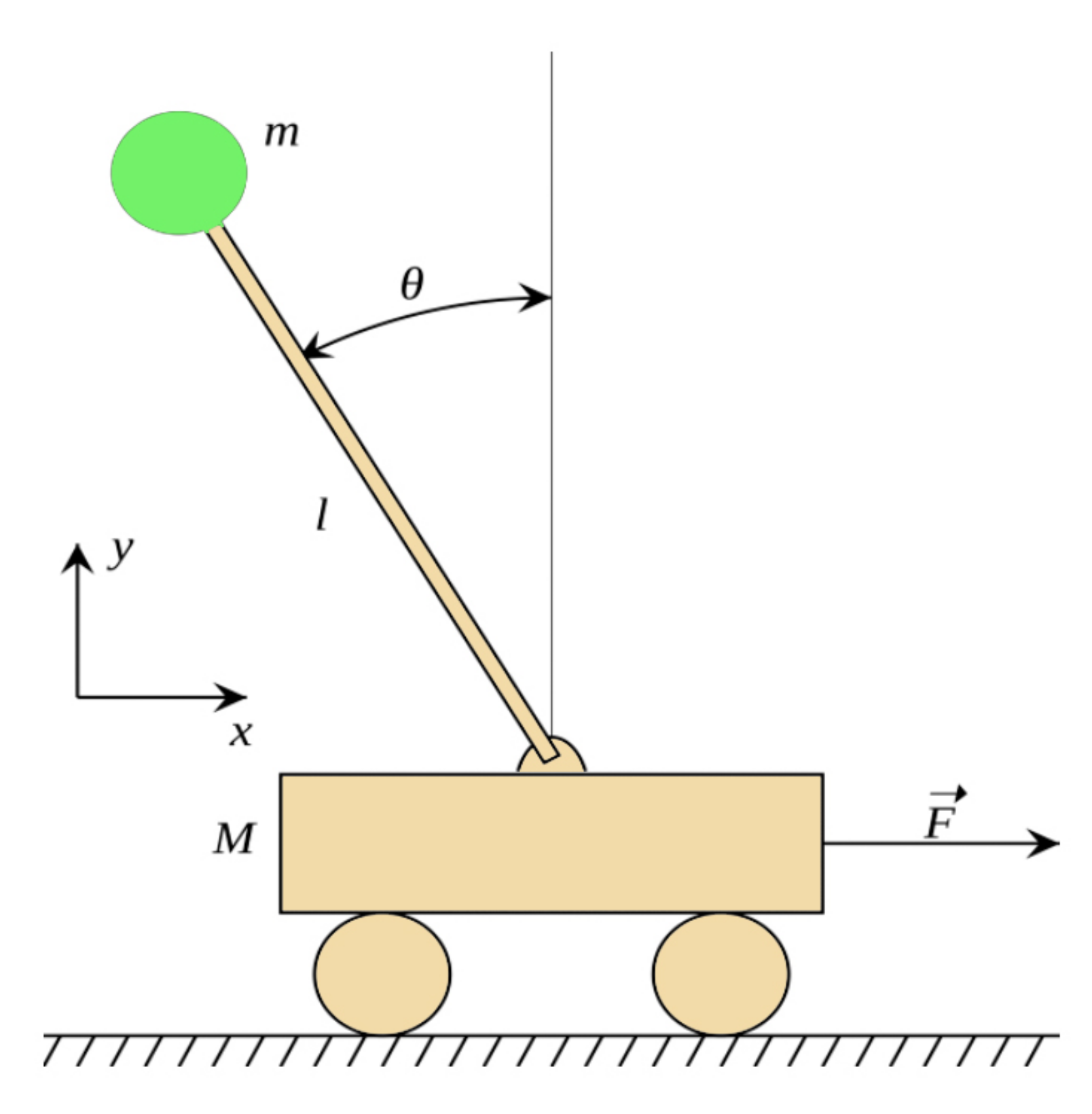
The pendulum equations are basically nonlinear; however, the proposed control method is presented for LPV systems. Therefore, to apply the proposed method, the nonlinear equations of pendulums or any other nonlinear systems in this class should first be expressed in the form of Equation (5). Below, we apply the proposed control method to an inverted pendulum (with exact equations) related to [32]. The inverted pendulum system is shown in Figure 1. The dynamic equations of an inverted pendulum are as follows:

$$\begin{array}{c}\ddot{\phi }\left(t\right)=\frac{gsin\left(\phi \left(t\right)\right)}{\frac{4L}{3}-\frac{a{m}_{p}L{cos}^2\left(\phi \left(t\right)\right)}{m_p+M_C}}-\frac{\frac{0.5a{m}_{p}L\dot{\phi }{\left(t\right)}^{2}sin\left(2\phi \left(t\right)\right)}{m_p+M_C}}{\frac{4L}{3}-\frac{a{m}_{p}L{cos}^2\left(\phi \left(t\right)\right)}{m_p+M_C}}-\frac{acos\left(\phi \left(t\right)\right)u\left(t\right)}{\frac{4L}{3}-\frac{a{m}_{p}Lcos\left(\phi \left(t\right)\right)}{m_p+M_C}}\hfill \end{array}$$

(58)

where $\phi \left(t\right),a,m_p,L,g$ are the angular displacement, the fixed number dependent on the pendulum mass and the cart mass ($M_c$), the pendulum length, and the gravitational acceleration, respectively. The values of a, $m_p$, L, and g are

$$2\le m_p\le 3,\frac{1}{19}\le a\le \frac{1}{10},g=9.81,L=0.5.$$

(59)

Considering the system modes as $X\left(t\right)={\left[x_1\left(t\right)x_2\left(t\right)\right]}^T={\left[\phi \left(t\right)\dot{\phi }\left(t\right)\right]}^T$, we can write

$$\begin{array}{c}{\dot{x}}_1=x_1\hfill \\ {\dot{x}}_2=f_1\left(X\left(t\right)\right)x_1\left(t\right)+f_2\left(X\left(t\right)\right)u\left(t\right)\hfill \end{array}$$

(60)

as

$$\begin{array}{c}{f}_1\left(X\left(t\right)\right)=\frac{g-\frac{a{m}_{p}L{x}_2{\left(t\right)}^{2}cos\left(x_1\left(t\right)\right)}{m_p+M_C}}{\frac{4L}{3}-\frac{a{m}_{p}L{cos}^2\left(x_1\left(t\right)\right)}{m_p+M_C}}\times \left(\frac{sin\left(x_1\left(t\right)\right)}{x_1\left(t\right)}\right)\hfill \end{array}$$

(61)

$$f_2\left(X\left(t\right)\right)=\frac{-acos\left(x_1\left(t\right)\right)}{\frac{4L}{3}-\frac{a{m}_{p}Lcos\left(x_1\left(t\right)\right)}{m_p+M_C}}$$

(62)

Finally, the inverse pendulum state equations are written in the following multidimensional form:

$$\dot{X}\left(t\right)=\sum _{i=1}^4{\theta }_i\left(t,\eta \right)\left(A_{i}X\left(t\right)+B_{i}u\left(t\right)\right)$$

(63)

where

$$\begin{array}{c}{\theta }_1\left(t,\eta \right)={\eta }_1\left(t,\eta \right)w_1\left(t,\eta \right)\hfill \\ {\theta }_2\left(t,\eta \right)={\eta }_1\left(t,\eta \right)w_2\left(t,\eta \right)\hfill \\ {\theta }_3\left(t,\eta \right)={\eta }_2\left(t,\eta \right)w_1\left(t,\eta \right)\hfill \\ {\theta }_4\left(t,\eta \right)={\eta }_2\left(t,\eta \right)w_2\left(t,\eta \right)\hfill \end{array}$$

(64)

$$\begin{array}{c}{\eta }_1\left(t,\eta \right)=\frac{f_{1max}-f_1}{f_{1max}-f_{1min}}\hfill \\ {\eta }_2\left(t,\eta \right)=\frac{f_1-f_{1min}}{f_{1max}-f_{1min}}\hfill \end{array}$$

(65)

$$\begin{array}{c}{w}_1\left(t,\eta \right)=\frac{f_{2max}-f_2}{f_{2max}-f_{2min}}\hfill \\ w_2\left(t,\eta \right)=\frac{f_2-f_{2min}}{f_{2max}-f_{2min}}\hfill \end{array}$$

(66)

In this case, the $\eta$ vector contains parameters a and $m_p$. The range for these parameters is $2\le m_p\le 3,\frac{1}{19}\le a\le \frac{1}{10}$. In [32], the arbitrary values selected for a and $m_p$ are 1/19 and 3, respectively.

First, the main system is created using the selected values for the vector of parametric uncertainties. Inaccurate scheduling parameters are then generated. Then, for each value of the $x_1\left(t_0\right)$ and $x_2\left(t_0\right)$ modes at the moment $t=t_0$ and according to the intervals provided for the parameters a and $m_p$, the maximum and minimum values of the timing parameters will be obtained at the said moment. Due to the nonlinearity of these parameters, we have to divide the intervals related to a and $m_p$ into small gaps and then, step by step, obtain and store the values of the timer parameters. Finally, according to the obtained values, we calculate the minimum and maximum of these parameters, i.e, ${\theta }_i^L\left(t,\eta \right)$ and ${\theta }_i^U\left(t,\eta \right)$ at the moment $t=t_0$, and call them the lower and upper bounds of the variable with time, respectively. After that, the auxiliary parameters introduced in [32] will be obtained. These auxiliary parameters are defined as follows:

$${\underline{\theta }}_i=\frac{{\theta }_i^L\left(t\right)}{{\sum }_{i=1}^p{\theta }_i^L\left(t\right)+{\theta }_i^U\left(t\right)},{\overline{\theta }}_i=\frac{{\theta }_i^U\left(t\right)}{{\sum }_{i=1}^p{\theta }_i^L\left(t\right)+{\theta }_i^U\left(t\right)}$$

(67)

Finally, the mode feedback gain will be calculated. The number of corners in the inverse view of the inverse pendulum system is equal to 4. Therefore, we will have eight auxiliary parameters. A total of four auxiliary parameters will be generated by ${\theta }_1^L\left(t,\eta \right),{\theta }_2^L\left(t,\eta \right),{\theta }_3^L\left(t,\eta \right),{\theta }_4^L\left(t,\eta \right)$ and another four auxiliary parameters will be generated by ${\theta }_1^U\left(t,\eta \right),{\theta }_2^U\left(t,\eta \right),{\theta }_3^U\left(t,\eta \right),{\theta }_4^U\left(t,\eta \right)$. As a result, the final auxiliary parameters are:

$${\overline{\theta }}_1\left(t,\eta \right),{\overline{\theta }}_2\left(t,\eta \right),{\overline{\theta }}_3\left(t,\eta \right),{\overline{\theta }}_4\left(t,\eta \right),{\underline{\theta }}_1\left(t,\eta \right),{\underline{\theta }}_2\left(t,\eta \right),{\underline{\theta }}_3\left(t,\eta \right),{\underline{\theta }}_4\left(t,\eta \right)$$

(68)

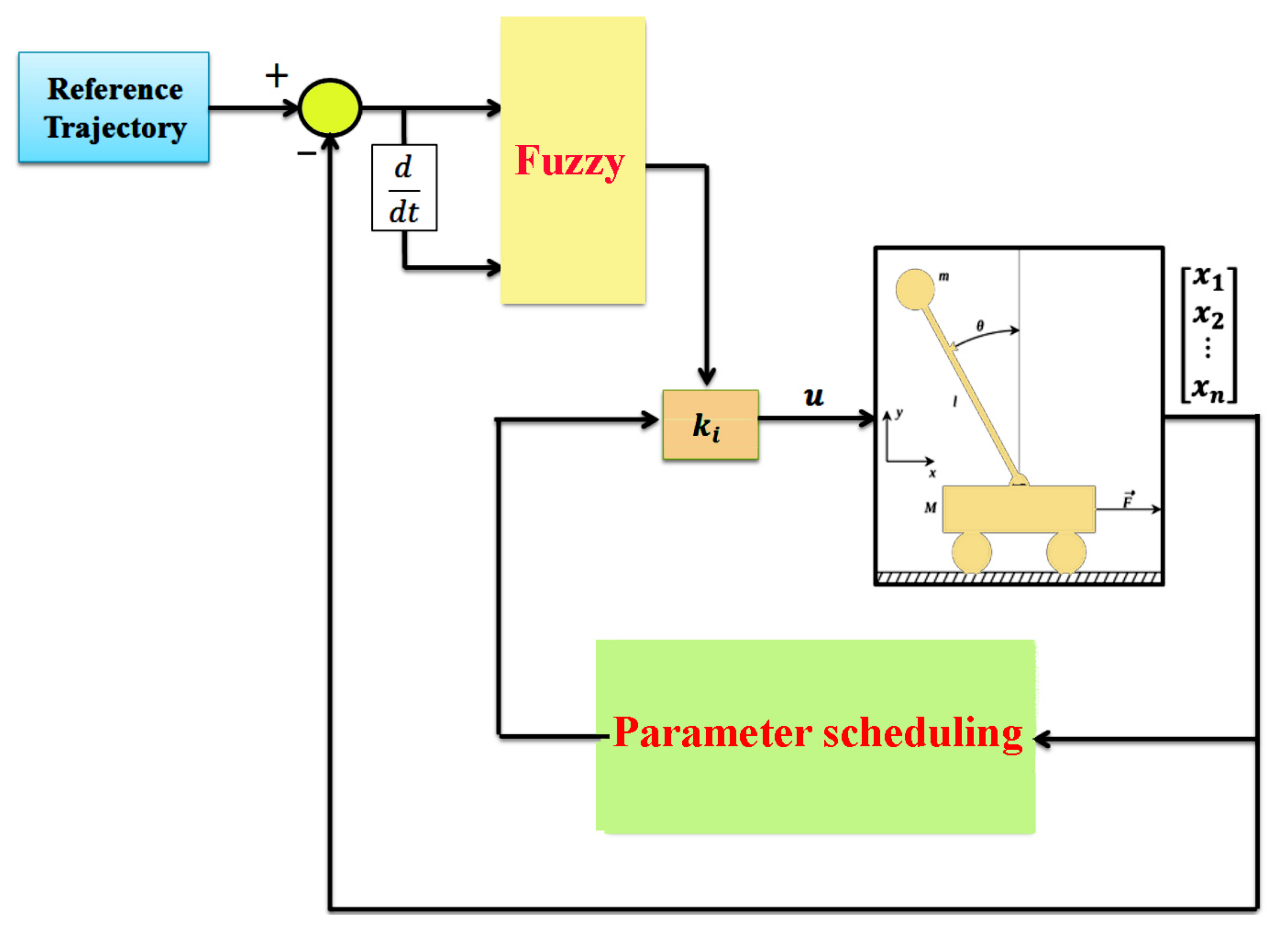
Figure 2 shows the structure of the control system. As seen in Figure 2, the gain-scheduling control system calculates $\theta$ parameters by taking feedback from the system states and after multiplying by $k_i$ gain, they are applied as a control signal to the pendulum system. The fuzzy system also has the task of calculating the gain at every moment according to the error of the states from their desired values. 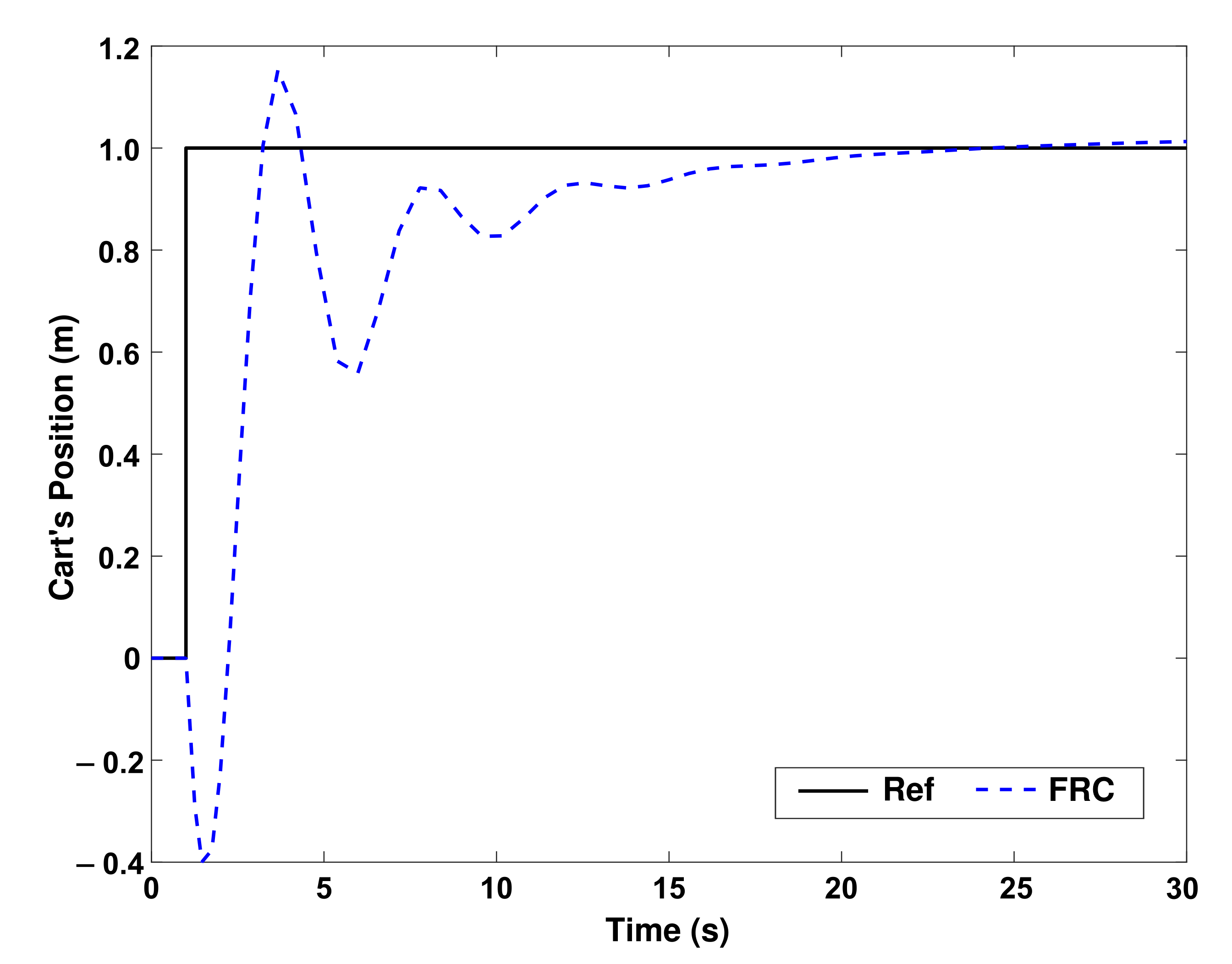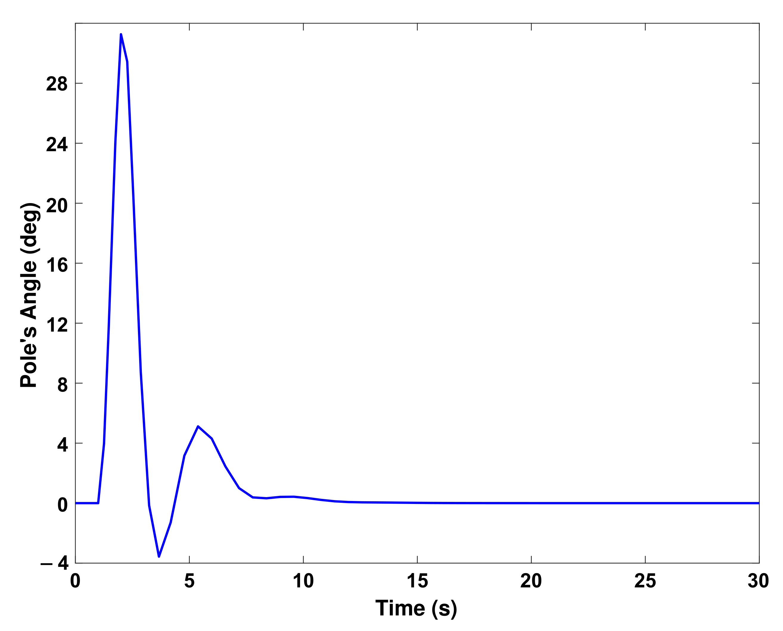As can be seen from [32], its method has led to an increase in computation, which is a major challenge in operational applications. This has led the authors in the case of [32] to confine themselves to computer simulation and not to carry out operational implementation. 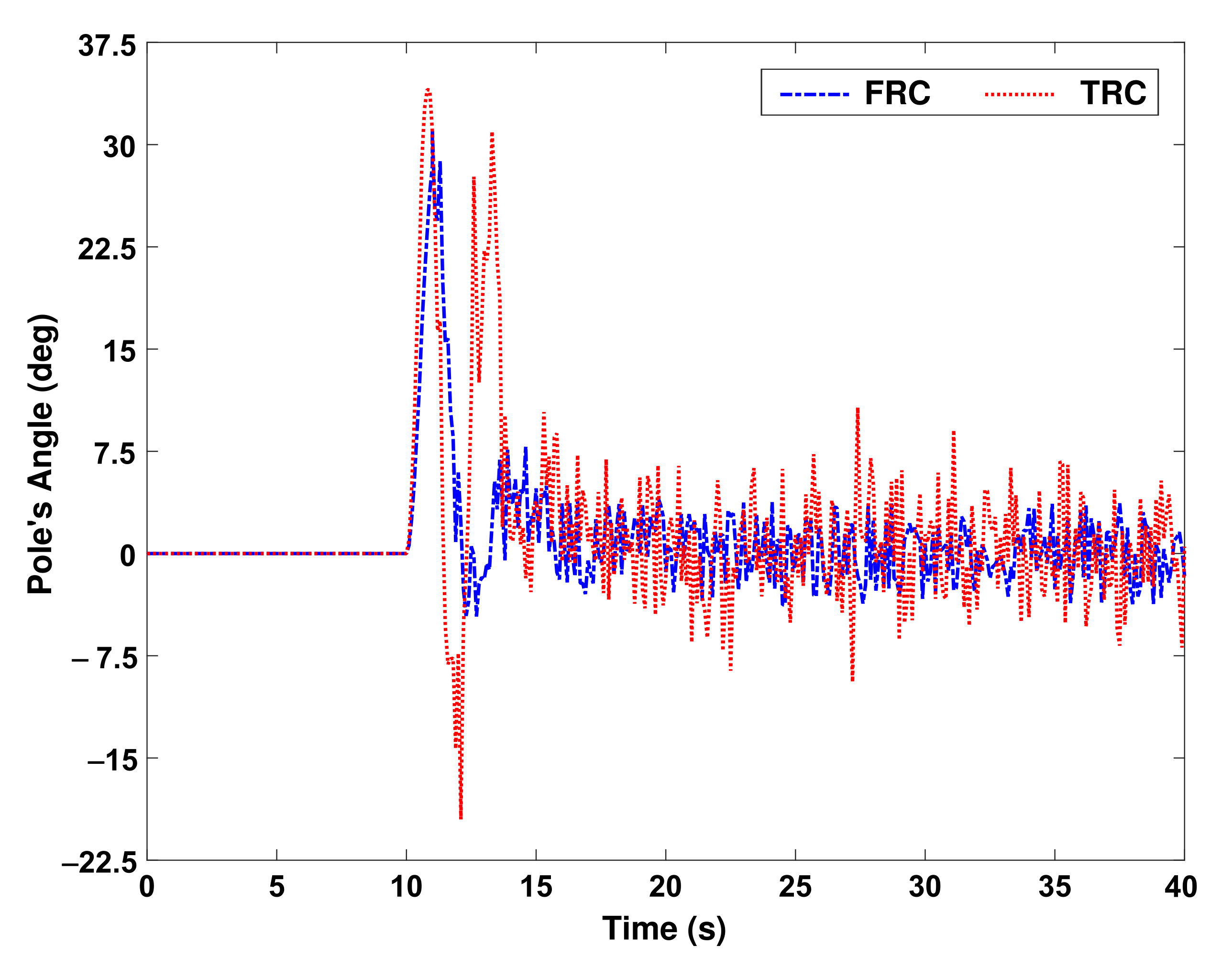However, the approach presented in [32] (which we called TRC) is applied to the inverted pendulum, and its simulation results are compared with the proposed method herein. The step response of the cart’s position and pole’s angle using the proposed method (FRC) is shown in Figure 3 and Figure 4, respectively.

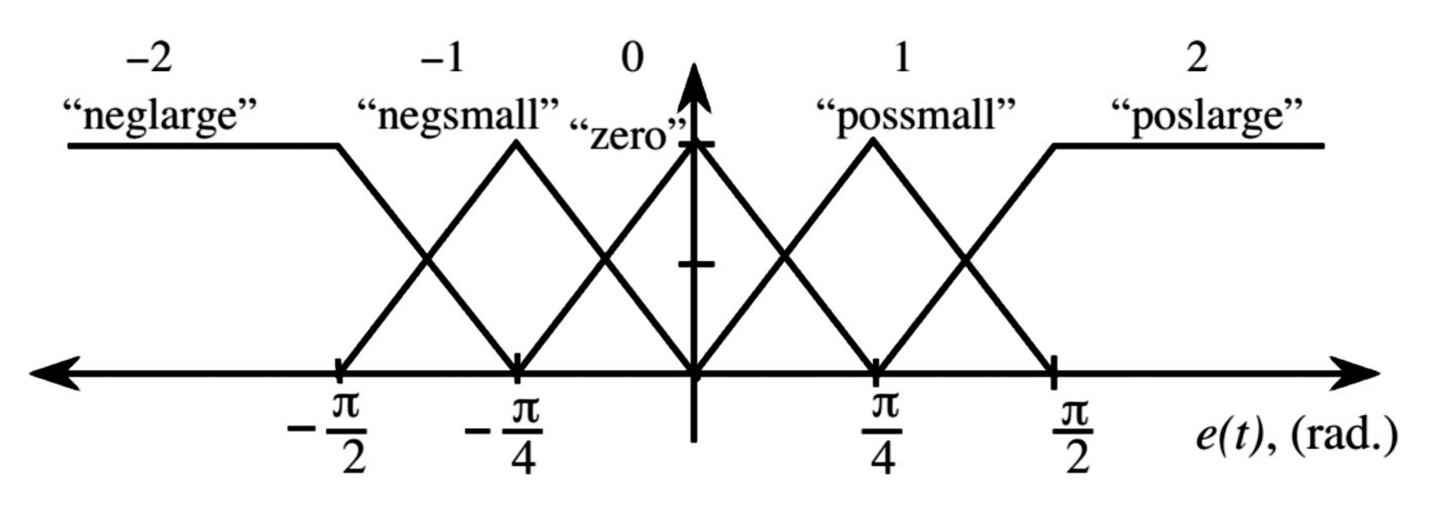
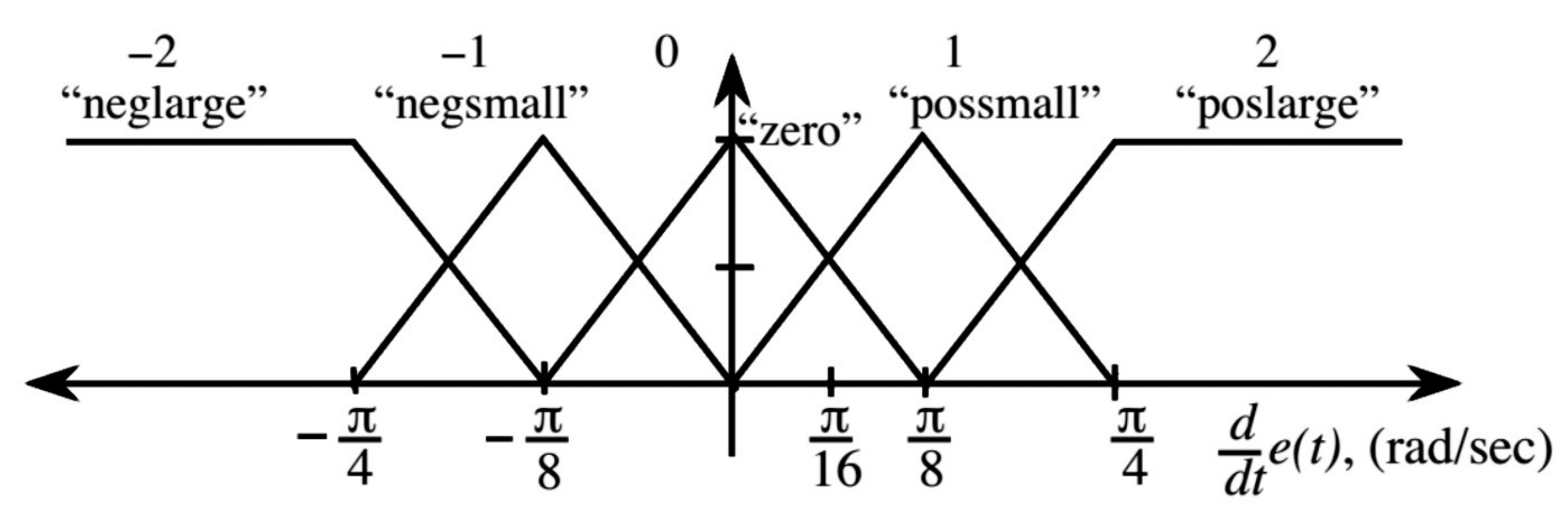
Note that $e\left(t\right)$ is the error between reference trajectory and actual output and $A_j$, $B_j$, and $C_j$ are fuzzy sets. Fuzzy sets can be triangular, Gaussian, trapezoidal, etc. The parameters of these sets are adjusted by an expert according to the error values. Triangular fuzzy sets are used in this article. For the error signal, five membership functions are considered as shown in Figure 5. 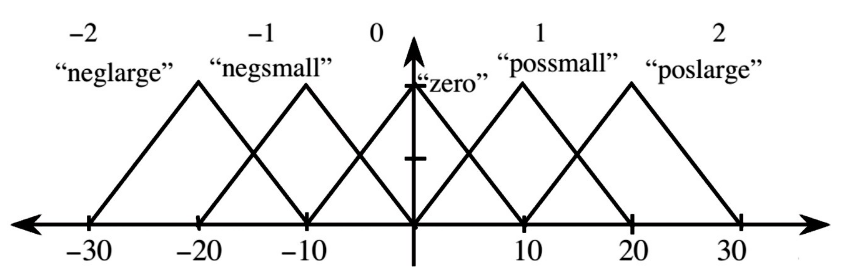Moreover, for error changes (or error derivative), the fuzzy sets are considered as Figure 6. Finally, the fuzzy membership functions for the output of the fuzzy control system (here $k_i$) are shown in Figure 7. The fuzzy rule base is given in

Table 1. The fuzzy rule base.

		$\dot{\mathit{e}}$
		−2	−1	0	1	2
e	−2	2	2	2	1	0
	−1	2	2	1	0	−1
	0	2	1	0	−1	−2
	1	1	0	−1	−2	−2
	2	0	−1	−2	−2	−2

. The procedure is as follows: first, the error and its derivative are determined for each of the membership functions, then the appropriate output is calculated by referring to the rule base table. To read more about the fuzzy system, see [33].

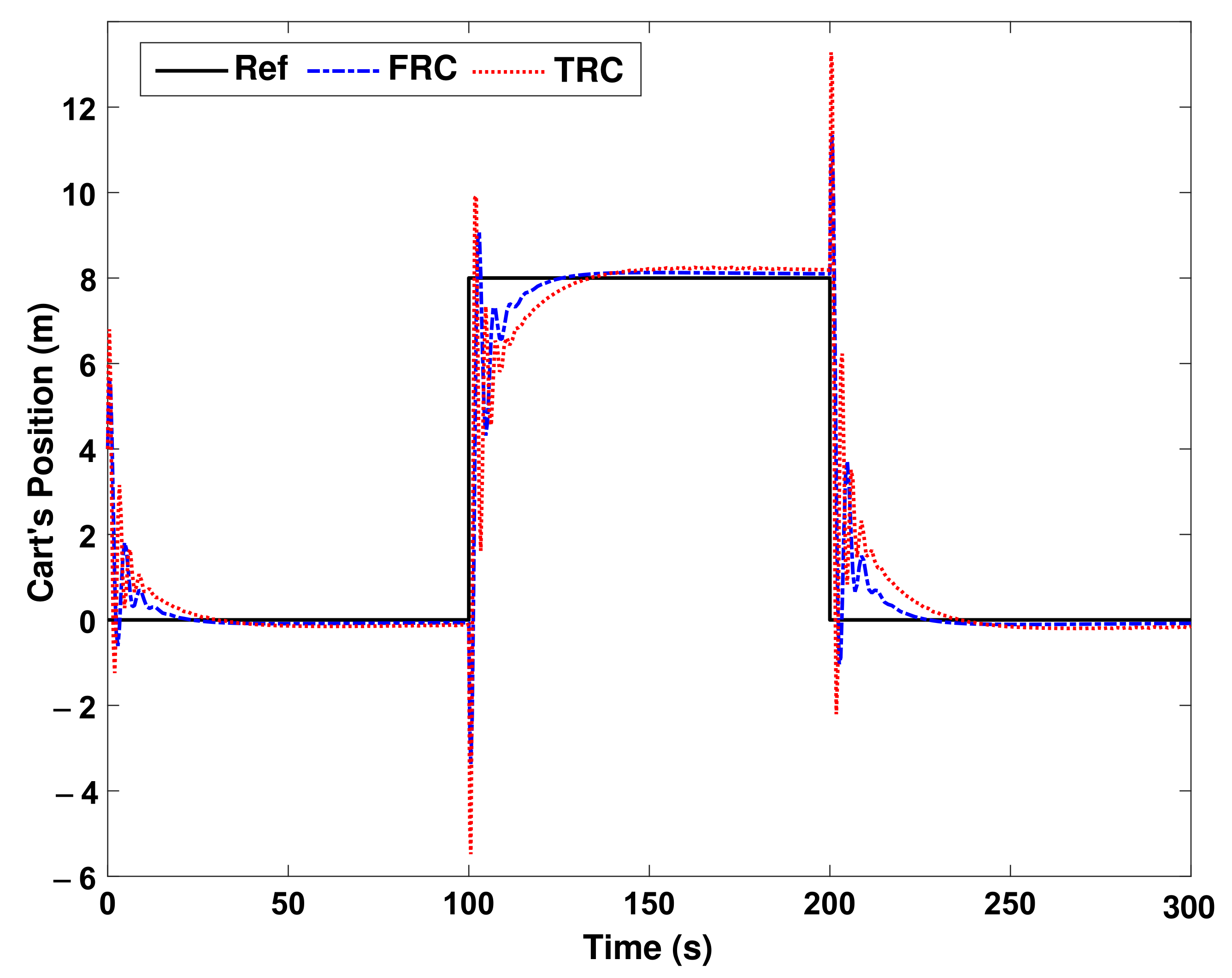
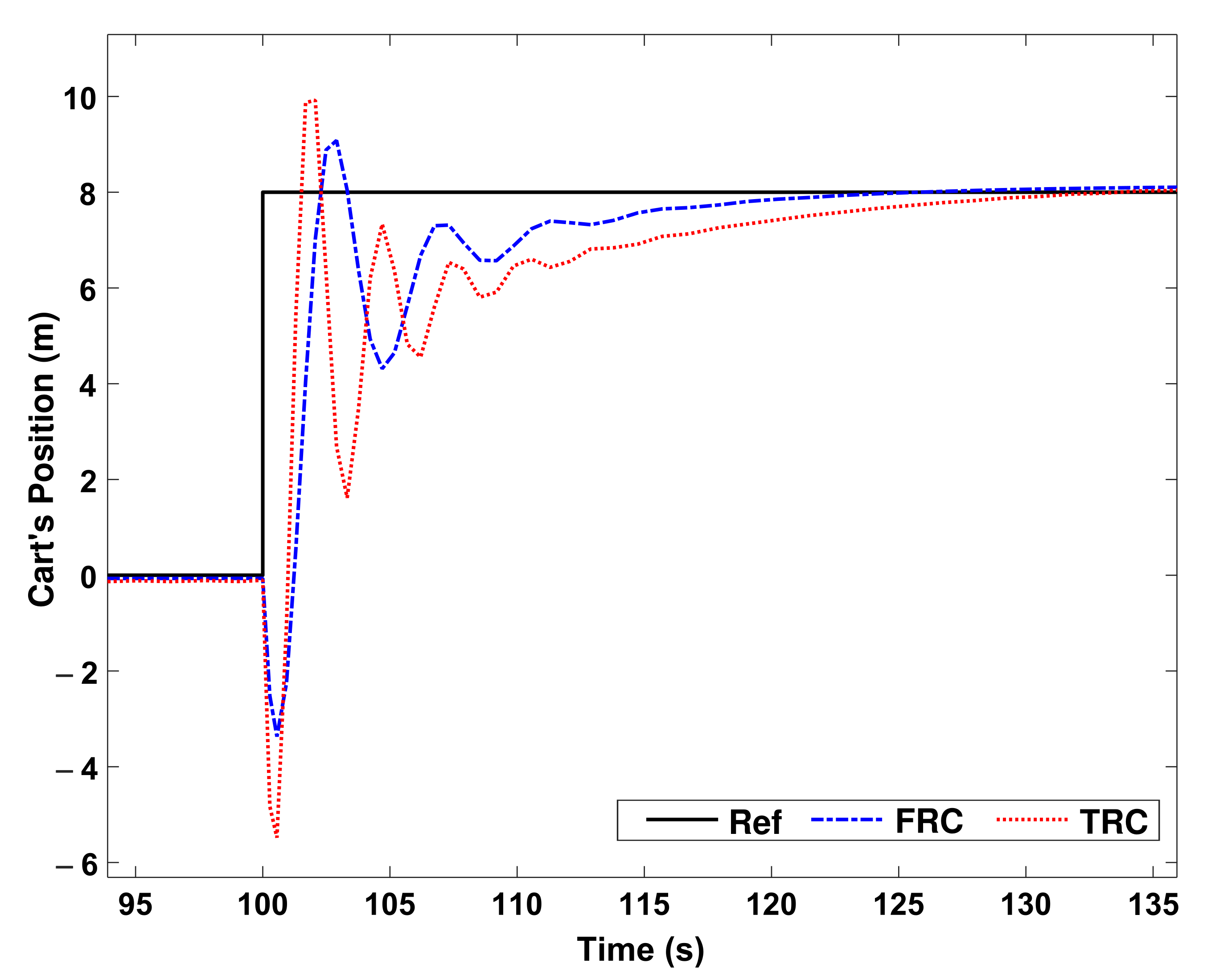
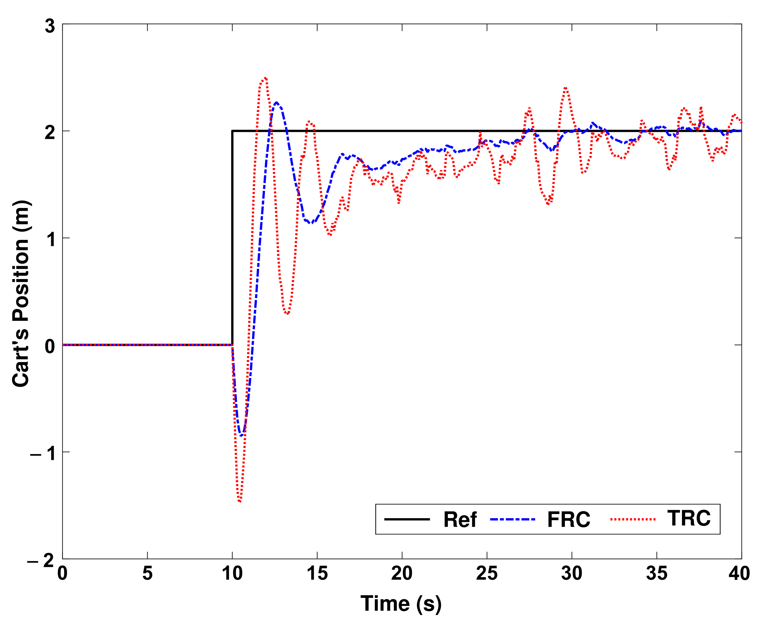
As the first scenario, assume that the system has gone from the origin to point $x=-2$ m, and then at $t=100$ s, the cart moves from $x=-2$ m to $x=2$ m, then at $t=200$ s, it moves from $x=2$ m to $x=-2$ m. Figure 8 shows the performance of the proposed fuzzy robust control (FRC) and traditional robust control (TRC) for cart’s position. For more clarity, in Figure 9, a portion of Figure 8 is magnified.

Figure 10 illustrates the results of angle control by FRC and TRC, and Figure 11 shows a magnified section of Figure 10.

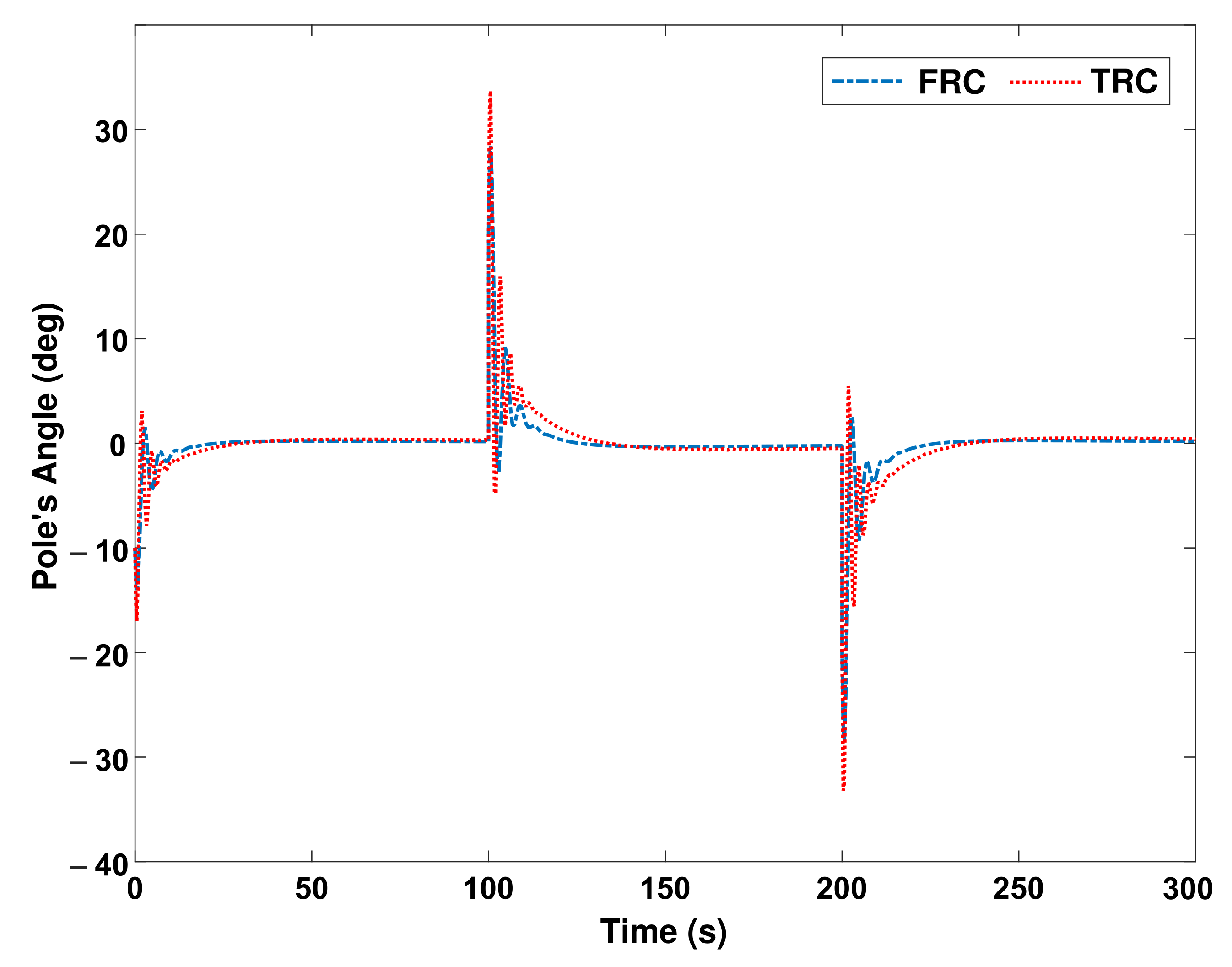
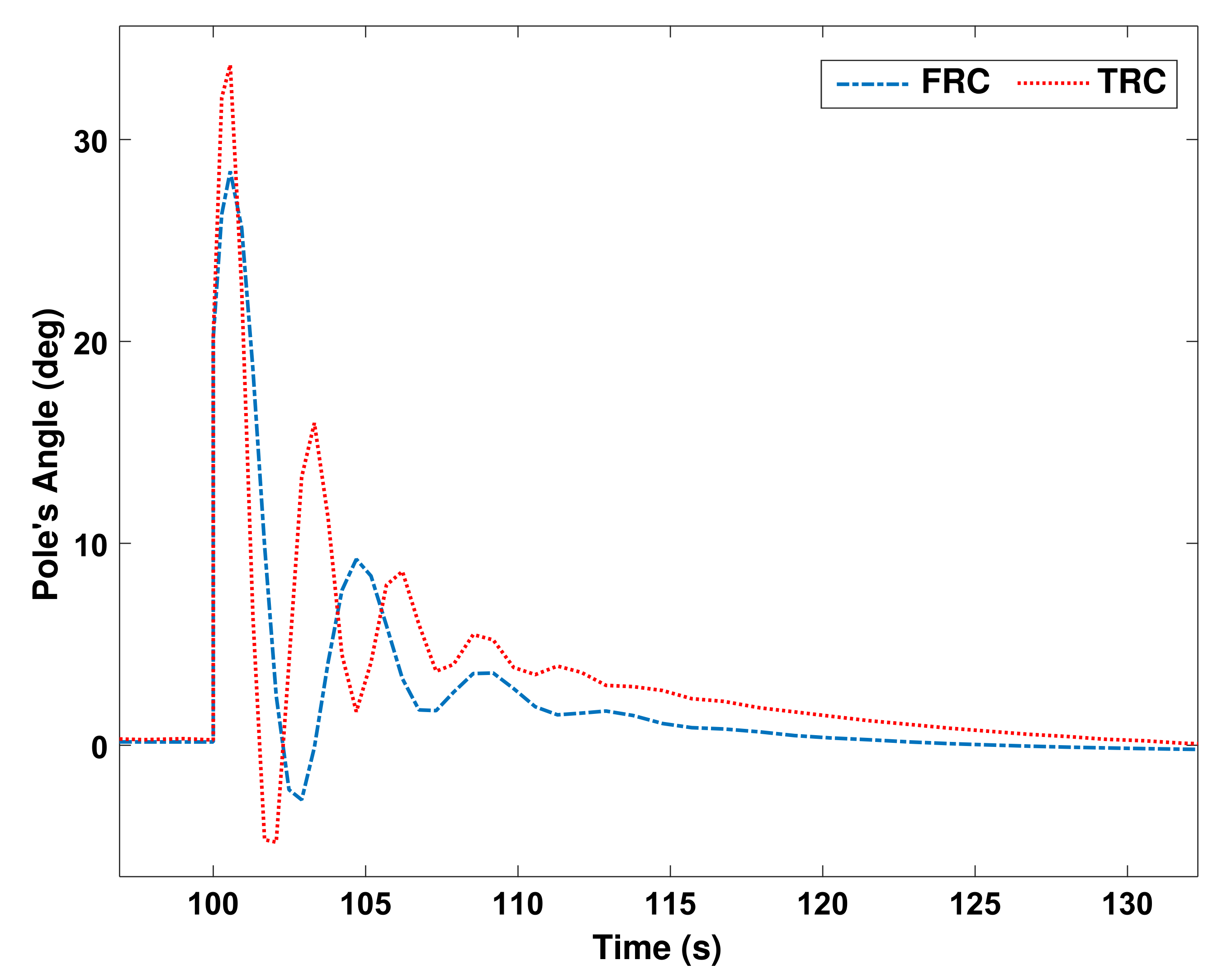
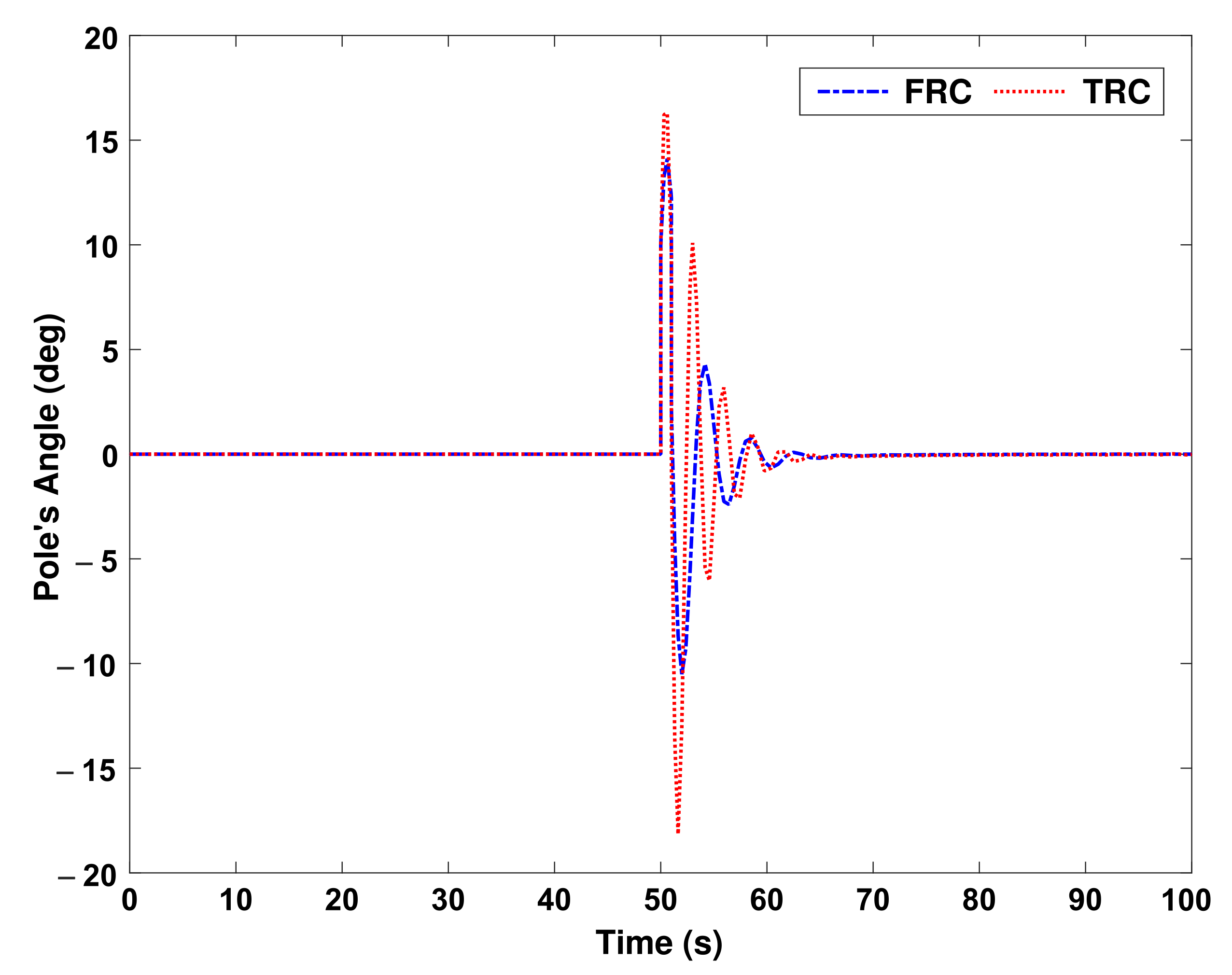
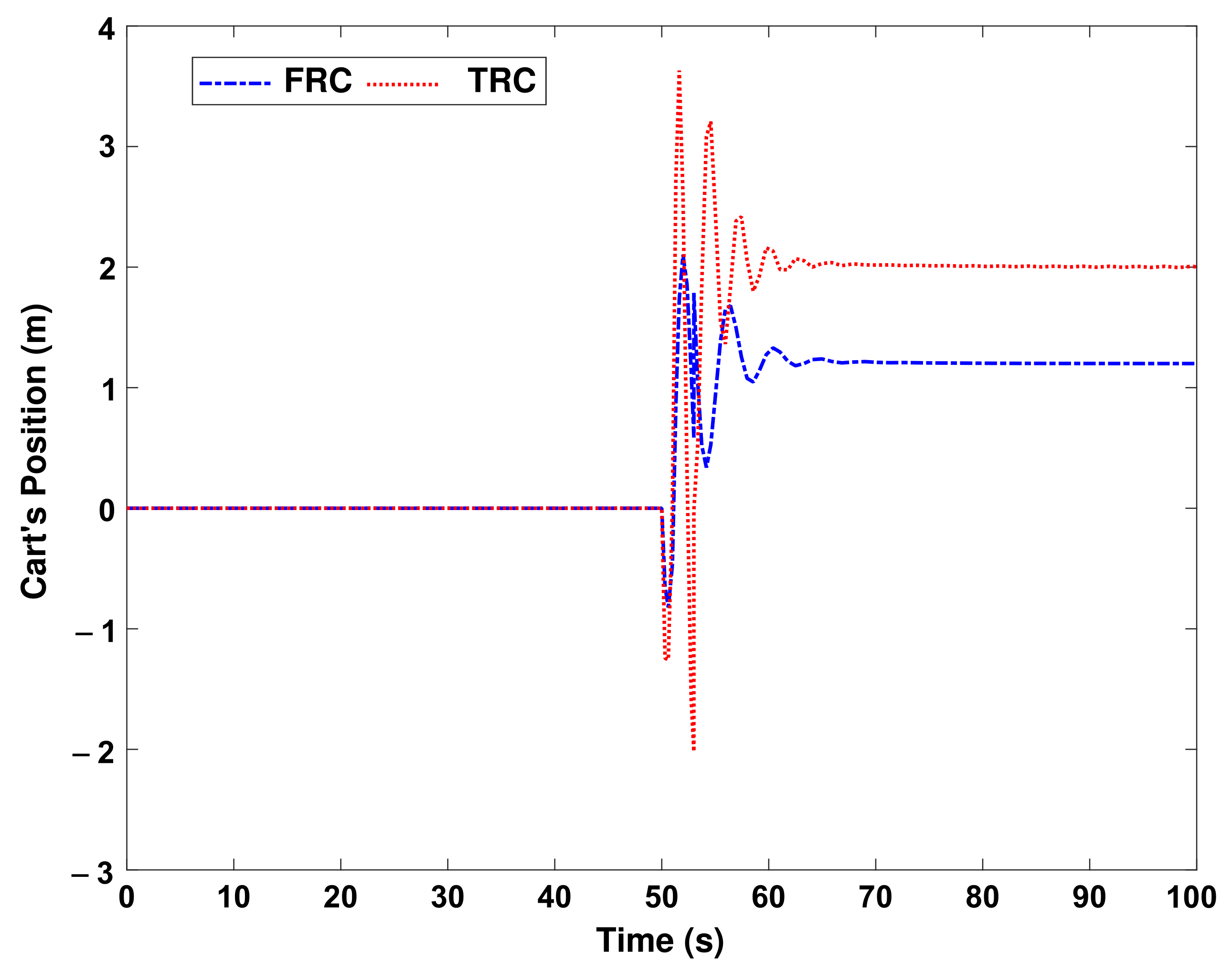
In order to challenge the control system, it is assumed that at $t=50$ s, a force equal to 1 Newton is applied to the pendulum at one moment. The control system should immediately prevent the pendulum from falling by moving the cart. Figure 12 shows the performance results of both control systems.

Figure 13 shows the performance of both control systems in moving the cart to maintain the balance of the pendulum. Another challenge of all control systems is the existence of uncertainty. Uncertainty is usually found in the value of parameters. We assume that the parameters of the pendulum system, such as the mass and length of the pendulum, the mass of the cart, and the coefficient of the friction between the trolley and the track, can change 10% of their nominal values. In Figure 14 and Figure 15, an indeterminate parameter is applied to the system from the moment $t=10$ s onward.

As it is clearly seen in Figure 14 and Figure 15, in the face of uncertainty, the performance of the FRC is more obvious than the TRC, and the reason for this superiority is due to the nature of fuzzy systems that have uncertainty in them.

State feedback is a common and efficient method to stabilize and control systems whose dynamics are nonlinear functions of system states. However, the efficiency of this method is challenged when the nonlinear functions are not accurate, or the dynamics of the system change under different conditions. In order to solve this problem, the gain of the state feedback can be considered adaptive (variable). This gain can be updated in different ways, including by a fuzzy system, neural network, or other evolutionary algorithms. However, the solution suggested in this article is to convert the nonlinear system into an LPV system.

6. Discussion

As we stated in the text of the article, the ${\eta }_{New}$ vector contains as that ${\eta }_{imin},{\eta }_{imax},i=1,2,\dots ,p$ are the values of the parametric uncertainties that minimize and maximize the $-i$ parameter of indefinite timing, respectively. In other words, first out of line and according to the interval of change of the system modes and the interval related to the parametric uncertainties, the values of uncertainties are obtained that minimize the indefinite timing parameters at all times. The calculated values are denoted by ${\eta }_{imin}$ and ${\eta }_{imax}$. Therefore, we do not need to calculate the minimum and maximum scheduling parameters moment by moment. For this reason, there is no need to create duplicate on-line computational loops, and the overall computational time will be greatly reduced. Then, by replacing the existing parametric uncertainties in the indefinite timing parameters with the values obtained and using a special idea (which is expressed in the introduction of the new timing parameters in the text of the current article), new timing parameters will be created. According to Equations (12) and (13), the new scheduling parameters will be as follows:

$${\theta }_{iNew}\left(t\right)=\frac{a_i\left(t\right)}{b\left(t\right)}i=1,2,3,4,\dots$$

(69)

$$\begin{array}{c}{a}_i\left(t\right)=3{\theta }_i\left(t\right)\left|{}_{\eta ={\eta }_{imin}}\right.+3\left({\theta }_i\left(t\right)\left|{}_{\eta ={\eta }_{imax}}+1\right.\right)-\hfill \\ {\displaystyle \sum _{\begin{array}{c}j=1\\ j\ne i\end{array}}^4\left({\theta }_i\left(t\right)\left|{}_{\eta ={\eta }_{jmax}}-1\right.\right)+\frac{1}{3}\sum _{\begin{array}{c}j=1\\ j\ne i\end{array}}^4\sum _{\begin{array}{c}\ell =1\\ \ell \ne j\end{array}}^4\left({\theta }_j\left(t\right)\left|{}_{\eta ={\eta }_{\ell max}}\right.\right)}\hfill \end{array}$$

(70)

$$b\left(t\right)=3\left(\sum _{q=1}^4{\theta }_q\left(t\right)\left|{}_{\eta ={\eta }_{qmax}}\right.+\sum _{q=1}^4{\theta }_q\left(t\right)\left|{}_{\eta ={\eta }_{qmin}}\right.+\sum _{q=1}^{4}2+1/3\right)$$

(71)

where

$$\begin{array}{c}{\eta }_{1max}=\left[0.13\right],{\eta }_{1min}=\left[0.0522\right]\hfill \\ {\eta }_{2max}=\left[0.13\right],{\eta }_{2min}=\left[0.0522\right]\hfill \\ {\eta }_{3max}=\left[0.0523\right],{\eta }_{3min}=\left[0.13\right]\hfill \\ {\eta }_{4max}=\left[0.0523\right],{\eta }_{4min}=\left[0.13\right]\hfill \end{array}$$

(72)

7. Conclusions

This article presented a new control system based on fuzzy logic for LPV systems. In this method, a fuzzy system calculates the feedback gain for the controller. The controller is based on a set of new scheduling parameters and is resistant to the usual parametric uncertainties with time-based specific intervals. Moreover, the asymptotic stability conditions of the closed-loop system were presented as linear matrix inequalities. An inverted pendulum system was investigated and controlled to evaluate the proposed method in the simulation section. The most critical challenge of the robust control system is determining the feedback gain, which was performed by trial and error in the traditional methods (TRC) and by a fuzzy system (FRC) in the proposed method. In the face of disturbance (the application of external force) and parametric uncertainty, the FRC method showed its proper efficiency. The proposed method can be used for controlling any systems in the form of Equation (5). As suggestions to continue the work, type-2 and type-3 fuzzy systems can be used.