Rock Burst Intensity Classification Prediction Model Based on a Bayesian Hyperparameter Optimization Support Vector Machine

Abstract

Rock burst disasters occurring in underground high-stress rock mass mining and excavation engineering seriously threaten the safety of workers and hinders the progress of engineering construction. Rock burst classification prediction is the basis of reducing and even eliminating rock burst hazards. Currently, most of mainstream discriminant models for rock burst grade prediction are based on small samples. Comprehensive selection according to many pieces of literature, the maximum tangential stress of surrounding rock and rock uniaxial compressive strength ratio coefficient (stress state parameter), rock uniaxial compressive strength and uniaxial tensile strength ratio (brittleness modulus), and the elastic energy index are used as a grading evaluation index of rock burst based on the collection of different construction engineering instances of rock burst in 114 groups of extensive sample data in different regions of the world, which are used to carry out the training study. The representativeness and accuracy of the index selection were verified by the indicator variance analysis and Spearman correlation coefficient hypothesis test. The Intelligent Rock burst Identification System (IRIS) based on an optimizable SVM model was established using data set samples. After extensive data cross-validation training, the accuracy of the SVM discriminant analysis model can reach 95.6%, which is significantly better than the prediction accuracy of the traditional SVM model of 71.9%. The model is used to classify and predict the rock burst intensity of 10 typical projects at home and abroad. The prediction results are consistent with the actual rock burst intensity, which is better than the discriminant model based on small sample data and other existing prediction models. The application of engineering examples shows that the results of the rock burst intensity classification prediction model based on extensive sample data processing analysis and the SVM discriminant method are in good agreement with the actual rock burst intensity, which can effectively provide a reference for the prediction of rock burst intensity grade in a construction area.

1. Introduction

Rock burst is a failure phenomenon in excavating underground rock mass with high stress. Under the action of excavation or other load disturbances, hard and brittle surrounding rocks in a high-stress state rapidly release the accumulated elastic energy, resulting in the dynamic instability disaster of rock spalling, fragmentation and ejection. Rock burst is characterized by its sudden occurrence and the significant harm caused, which not only poses a significant threat to the construction personnel and mechanical equipment, but also delays the construction period, even destroying the whole project and inducing earthquakes [1]. On 28 November 2009, an intense rock burst occurred in the drainage tunnel of Jinping Ii Hydropower Station, resulting in seven deaths and direct economic losses of hundreds of millions of CNY [2]. On 9 March 2014, a rock collapse caused by a rock burst occurred in the Dulong River highway tunnel in Gongshan, Yunnan province, killing three construction workers [3]. With the development of mining activities to a great depth, the increase of buried depth and the increase in stress level, the mining and excavation of underground high-stress rock mass shows a sudden trend of high frequency.

The accurate grading prediction of rock burst intensity has an extremely important theoretical and practical status for the effective prevention and control of rock burst in engineering. In general, rock burst prediction methods can be divided into four categories [4], namely the rock burst criterion method, numerical index method, applied mathematical method and on-site monitoring method. With the continuous development of big data analysis technology, the nonlinear rock burst prediction method (applied mathematical method) that comprehensively considers multiple influencing factors has achieved good rock burst prediction results and is a method with good development prospects in future rock burst intensity prediction. In particular, the typical “training modeling” method can achieve a better prediction effect. The main idea is that a fixed number of rock burst instance samples were trained and taught to establish a prediction model, including the neural network method, support vector machine (SVM) method, Distance discriminant method, Bayes discriminant method, Fisher discriminant method, Gaussian process method, random forest model and many other methods, but some machine learning algorithms have shortcomings in their application process. For example, Naive Bayes [5] has a poor classification effect on sample data sets with a strong index correlation. After testing, the accuracy of the prediction method is stable at 79.8%. The classification effect of random forest on low-dimensional data is not good, and the accuracy of the prediction method is stable at 79.8% after testing. Neural network [5] has a slow convergence speed in the learning process, and the hidden layer neurons need to be selected. After testing, the accuracy of this prediction method is stable at 86.8%. Due to the randomness and complexity of rock burst disasters, it is necessary to select a discriminant model with a good learning effect and high prediction accuracy.

In practical application, the optimized SVM algorithm is better than the traditional SVM algorithm in all aspects, which provides a way to solve the problem of SVM being difficult to calculate and classify large-scale training samples. The advantage of the optimizable SVM algorithm in the training process lies in that it can optimize and adjust the multi-class methods, box constraint level, kernel function, kernel scale and standardized data in the hyperparameter training process in the iterative process until the best classification effect is obtained. Based on the above analysis, the optimized SVM classification prediction model was established and applied to 132 groups of typical rock burst samples for training and testing. The model was compared with XGBoot (the accuracy is stable at 70%), RF (the accuracy is stable at 70%) and SVM models (the accuracy is stable at 80%) in engineering applications, which proved the accuracy, reliability and practicability of the optimized SVM discriminating model (the accuracy is stable at 95.6%).

2. Principle and Method of Rock Burst Intensity Prediction Model

Support Vector Machines (SVM) are a linear classifier model developed in the late 20th century to solve the binary classification problem. They map the feature vectors of the study samples to some points in the space through a specific rule. Their purpose is to draw the distinction line between the two. To distinguish the two kinds of topics accurately and efficiently, even after the training is completed, new issues to be measured are added, and the trained lines can still be classified well. The key to the SVM machine learning algorithm is to select the kernel function and related parameters of the model. Standard kernel functions include the linear kernel function, radial basis kernel function, Laplacian kernel function, and so on. With little subjective influence, this method is one of the most commonly used classifiers with the best effect at present. Since its optimization goal is to minimize structural risk, it has excellent generalization ability, so it has been widely used in the classification and prediction of rock burst intensity. Based on collecting a large number of rock burst samples, the SVM discriminant model for rock burst intensity classification prediction is established and applied in engineering.

2.1. Support Vector Machines

Support Vector Machines (SVM) are a linear classifier model developed in the late 20th century to solve the binary classification problem. They map the feature vectors of the study samples to some points in the space through a specific rule. Its purpose is to draw the distinction line between the two. To distinguish the two kinds of topics accurately and efficiently, even after the training is completed, new issues to be measured are added, and the trained lines can still be classified well. The key to the SVM machine learning algorithm is to select the kernel function and related parameters of the model. Standard kernel functions include the linear kernel function, radial basis kernel function, Laplacian kernel function, and so on. With little subjective influence, this method is one of the most commonly used classifiers with the best effect at present. Since its optimization goal is to minimize structural risk, it has excellent generalization ability, so it has been widely used in the classification and prediction of rock burst intensity. Based on collecting a large number of rock burst samples, the SVM discriminant model for rock burst intensity classification prediction is established and applied in engineering.

(1)

Linear Support Vector Machines. According to the principle of the SVM hyperplane $w\times x+b=0$ to divide the sample data set, to ensure the maximum classification interval, the hyperplane optimization method is expressed as Formula (1)

$$min\vartheta \left(w\right)=\frac{1}{2}{\left|\left|w\right|\right|}^2=\frac{1}{2}{w}^{T}w$$

(1)

Lagrangian functions are usually used to convert samples of initial problems into dual problems, resulting in Formula (2).

$$max\mu \left(a\right)={\displaystyle \sum }_{i=1}^n{a}_i-\frac{1}{2}{\displaystyle \sum }_{i,j=1}^n{a}_i{a}_j{y}_i{y}_j\left(x_i\times x_j\right)$$

(2)

After solving by Formula (2), the optimal classification function can be obtained by Formula (3)

$$f\left(x\right)=sgn\left(w^T+b\right)=sgn({\displaystyle \sum }_{i=1}^n{a}_i^{*}{y}_i\left(x_i\times x\right)+b^{*})$$

(3)

However, in practical application, many data samples are linearly indivisible, so blindly using the linearly inseparable method causes significant errors. To deal with this situation, the problem adaptation formula is changed into Formula (4) after the relaxation variable is introduced.

$$\vartheta \left(w\right)=\frac{1}{2}{\left|\left|w\right|\right|}^2+C{\displaystyle \sum }_{i=1}^n{ϵ}_i$$

(4)

where C is the penalty factor.

The Lagrange algorithm was used to solve the problem and Formula (5) was obtained.

$$max\mu \left(a\right)={\displaystyle \sum }_{i=1}^n{a}_i-\frac{1}{2}{\displaystyle \sum }_{i,j=1}^n{a}_i{a}_j{y}_i{y}_j\left(x_i\times x_j\right)$$

(5)

After solving all kinds of coefficients $a_i$, the classification decision function is obtained, and the Formula (6) is obtained.

$$f\left(x\right)=sgn({\displaystyle \sum }_{i=1}^n{a}_i^{*}{y}_i\left(x_i\times x\right)+b^{*})$$

(6)

(2)

Nonlinear Support Vector Machines. By the theorem of the Mercer condition for any symmetric function $K\left(x,\dot{x}\right)$, for any $\phi \left(x\right)\ne 0$ and $\int {\phi }^2\left(x\right)d_x<\infty$, existence $\iint K\left(x,\dot{x}\right)\phi \left(x\right)\phi \left(\dot{x}\right)d_x{d}_{\dot{x}}>0$ was established. The symmetry function $K\left(x,\dot{x}\right)$ is used to replace the inner product of the optimal classification plane, so the optimization function is Formula (7) (nonlinear data condition).

$$\mu \left(a\right)={\displaystyle \sum }_{i=1}^n{a}_i-\frac{1}{2}{\displaystyle \sum }_{i,j=1}^n{a}_i{a}_j{y}_i{y}_j\left(x_i\times x_j\right)$$

(7)

The classification decision function is transformed into Formula (8) (nonlinear data condition).

$$f\left(x\right)=sgn({\displaystyle \sum }_{i=1}^n{a}_i^{*}K\left(x_i\times x\right)+b^{*})$$

(8)

2.2. Bayesian Optimization

Based on Bayesian optimization of parameter tuning, in the traditional SVM model, including parameters C and other parts of the above parameters, these parameters and performance have the characteristics of the black-box model, namely between the version of the model and parameters that cannot use the expression to describe, only using the traversal method for construction of the optimal SVM model. Bayesian optimization [6] is an efficient optimization algorithm with sample validity mainly used for parameter tuning machine learning models. This method adopts the Gaussian process to establish a probability proxy model, refers to previous parameter information and iteratively updates prior knowledge, and can determine the optimal parameters of the model in a relatively short time. In general, the expression of the gaussian process is shown in Formula (9).

$$f\left(x\right)~GP\left[m\left(x\right),k\left(x,x^{\prime }\right)\right]$$

(9)

In Formula (9), the mean function $\left(x\right)=E\left(f\left(x\right)\right)$ represents the mathematical expectation of sample $f\left(x\right)$ and the covariance function $k\left(x,x^{\prime }\right)=E\left\{\left[f\left(x\right)-m\left(x\right)\right]\left[f\left(x^{\prime }\right)-m\left(x^{\prime }\right)\right]\right\}$. The gaussian process uses some known points to estimate the mean and variance of the objective function at other points. It then constructs the acquisition function to determine the location of sampling points in the iterative process.

2.3. The Intelligent Rock Burst Identification System

In this paper, Bayesian optimization is adopted as the parameter optimization algorithm of the SVM model. The specific algorithm (based on the Python language environment) flows as follows:

(1)

According to the principle of the SVM model, the value range of equation coefficients such as hyperparameter $C$ is determined and $n_0$ sampling points are randomly selected. The average accuracy of cross-validation is used as the objective function $f$, and the parameter combination of the model is used as the independent variable $x_0$ to construct a surrogate model, and the initial distribution of the objective function and the sampling point set $D$ are obtained.

(2)

Maximize the objective function to obtain the next sampling point $x_t$ and the function value $f\left(x_t\right)$.

(3)

Add sampling points $\left[x_t,f\left(x_t\right)\right]$ to set $D$, and synchronously update the Gaussian process surrogate model to further fit the distribution of the objective function.

(4)

Return to step (2) and continue the iteration until the algorithm iteration reaches the maximum number of iterations, and then output the optimal sampling point to obtain the optimal hyperparameter $C$ equivalent of the SVM model.

2.4. Great Advantages of Support Vector Machine Based on Bayesian Hyperparameter Optimization

Usually, the influence of a support vector machine is the main problem in building a model to fill in the necessary parameter values; these values are not limited to penalty factor and the parameters of the kernel function are set. Only relying on the existing provisions of researchers and the experience of related papers can lead to a support vector machine (SVM) in which the rock burst prediction accuracy is not huge, and parameter selection and the accuracy value are small. There is no improvement in accuracy; if the parameter selection and the accuracy value are large, it is impossible to judge whether the model result is overfitting. Which parameters to choose and how to choose the parameters are the problems that need to be solved urgently in support vector machine prediction.

The optimizable support vector machine (SVM) model, as a supervised learning algorithm, greatly eliminates the influence of the choice of penalty factor and kernel function on the classification performance of the SVM. The SVM algorithm can be optimized in the process of training; the advantage is that the limit parameters must be stipulated in advance, instead of in the process of model forecast adjustments, according to the classification of the real-time condition, as well as in the process of iteration for super parameters in the process of the training class method, box constraint level, kernel function, the nuclear scale, and standardized data optimization adjustment, until the best classification effect is obtained.

3. Index Selection and Variance Analysis of Rock Burst Intensity Prediction

3.1. Prediction Index Selection

The rock burst mechanism is complex and affected by many factors. This study is based on the characteristics of rock burst, the causes and the internal and external conditions, combining previous researchers’ experience, after a comprehensive analysis to determine the rock burst tendency prediction evaluation index as follows: (1) the maximum tangential stress of surrounding rock and rock uniaxial compressive strength ratio characterizes the surrounding rock stress and rock burst cavern; (2) the ratio of uniaxial compressive strength to the uniaxial tensile strength of rock represents the relationship between rock burst and lithology; (3) the elastic energy index represents the energy characteristics of the rock. Rock burst intensity can be divided into four categories: N (no rock burst activity), L (mild rock burst activity), M (moderate rock burst activity), and H (severe rock burst activity). Referring to the research results of Wang Yuanhan [7], the corresponding relationship between each evaluation index and rock burst intensity is shown in

Table 1. Prediction standard of rock burst tendency.

Index	Values at Each Rock Burst Level
	N	L	M	H
$\raisebox{1ex}{${\sigma }_{\theta }$}\!\left/ \!\raisebox{-1ex}{${\sigma }_c$}\right.$	0~0.3	0.3~0.5	0.5~0.7	>0.7
$\raisebox{1ex}{${\sigma }_c$}\!\left/ \!\raisebox{-1ex}{${\sigma }_t$}\right.$	>40	26.7~40	14.5~26.7	0~14.5
$W_{et}$	0~2	2~4	4~6	>6

.

3.2. Establish a Learning Sample Set

By referring to a large amount of literature and relevant materials [5,8], 132 typical rock burst samples were collected and sorted in this paper, and 18 unqualified examples were excluded (e.g., the intensity levels of models in different kinds of literature were inconsistent, etc.). The remaining 114 learning examples are from several projects at home and abroad; they include: Tianshengqiao secondary hydropower station, Longyangxia hydropower station, Lijiaxia hydropower station, Norway Heavy Metal Tunnel, Rail Lead-zinc sulfide mine in Italy, Qinling tunnel, Jiangbian Hydropower Station, Jinchuan No. 2 mine, Maluping mine, Beizhihe Iron Mine, Jinping Secondary power station, Cangling tunnel, Erlang Mountain tunnel, and so on. Specific data parameters of learning samples for rock burst intensity classification prediction are shown in

Table 2. Rock burst sample data and classification prediction results.

Sample Number	Classification Index			A L	P L	Sample Number	Classification Index			A L	P L
	$\raisebox{1ex}{${\mathit{\sigma }}_{\mathit{\theta }}$}\!\left/ \!\raisebox{-1ex}{${\mathit{\sigma }}_{\mathit{c}}$}\right.$	$\raisebox{1ex}{${\mathit{\sigma }}_{\mathit{c}}$}\!\left/ \!\raisebox{-1ex}{${\mathit{\sigma }}_{\mathit{t}}$}\right.$	${\mathit{W}}_{\mathit{e}\mathit{t}}$				$\raisebox{1ex}{${\mathit{\sigma }}_{\mathit{\theta }}$}\!\left/ \!\raisebox{-1ex}{${\mathit{\sigma }}_{\mathit{c}}$}\right.$	$\raisebox{1ex}{${\mathit{\sigma }}_{\mathit{c}}$}\!\left/ \!\raisebox{-1ex}{${\mathit{\sigma }}_{\mathit{t}}$}\right.$	${\mathit{W}}_{\mathit{e}\mathit{t}}$
1	0.34	24	6.6	M	M	58	0.57	25.6	3.8	M	M
2	0.11	31.2	7.4	N	N	59	0.61	25.6	3.7	M	M
3	0.1	23	5.7	N	N	60	0.56	29.2	4.8	M	M
4	0.42	21.7	5	M	M	61	0.71	32.2	5.5	H	H
5	0.77	17.5	5.5	H	H	62	0.49	49.5	4.7	M	M
6	0.4	14.7	7.1	M	M	63	0.46	45.5	5.2	M	M
7 *	0.54	14.2	6.2	H	M	64	0.47	55	5	M	M
8	0.4	15	7.1	M	M	65	0.31	42.8	1.8	N	N
9	0.58	13.2	6.3	H	H	66	0.61	25	3.7	M	M
10	0.2	36	2.3	N	N	67	0.55	31.3	4.6	M	M
11	0.19	47.9	1.9	N	N	68	0.69	32.1	5.9	H	H
12	0.66	13.2	6.8	H	H	69	0.5	50.9	5.2	M	M
13	0.4	15.6	3.5	L	L	70	0.69	16.9	3.4	M	M
14	0.44	13.1	2.1	L	L	71	0.42	17	10.9	H	H
15	0.13	6.7	1.4	N	N	72	0.3	20.4	5	L	L
16 *	0.37	24	5.1	L	M	73	0.54	12.2	4.9	M	M
17	0.45	11.2	2	L	L	74	0.2	11.2	3.6	N	N
18	0.19	6.7	1.4	N	N	75	0.35	22.7	3.3	L	L
19	0.48	24	5.1	M	M	76	0.72	13.9	9.1	H	H
20	0.74	24.4	6.3	H	H	77	0.64	14.4	7.7	H	H
21	0.23	6.7	1.4	N	N	78	0.47	16.5	5.5	M	M
22	0.61	24	5.1	M	M	79	0.52	18.6	4.2	M	M
23	1	11.2	2	H	H	80	0.45	14.8	3.1	L	L
24	0.28	9.7	1.9	N	N	81	0.2	14.1	3.6	N	N
25	0.7	11.7	2.8	M	M	82	0.55	11.1	4	M	M
26	0.11	27.2	7	N	N	83	0.56	16.3	3.3	M	M
27	0.13	18.8	3.6	N	N	84	0.41	30.7	4.3	L	L
28	0.1	21.4	4.7	N	N	85	0.22	9	4.9	L	L
29	0.67	26.8	0.9	L	L	86	0.45	6.8	2.2	L	L
30	0.83	28.9	3.2	M	M	87	0.28	9.5	6.1	M	M
31	0.93	28.9	3.2	H	H	88	0.35	12.1	2.9	L	L
32	0.74	28.9	3.2	M	M	89	0.66	22.3	3.2	M	M
33	1.41	19.2	3.1	H	H	90	0.72	13.2	5.2	H	H
34	0.79	22	2	M	M	91	0.37	29.7	3.5	L	L
35	0.56	20.4	2	L	L	92	0.42	32.8	3	L	L
36	0.46	20.4	2	L	L	93	0.28	42.7	2.2	N	N
37	0.49	19.7	2.3	L	L	94	0.38	28.8	3	L	L
38	0.44	19.7	2.3	L	L	95	0.72	27.5	4.3	M	M
39	0.84	19.7	2.3	M	M	96	0.69	16.6	5.7	H	H
40	0.42	19.7	2.3	L	L	97	0.42	15.5	3.2	L	L
41	0.46	19.7	2.3	L	L	98	0.22	36.4	1.8	N	N
42	0.28	23.6	4.9	L	L	99	0.62	19.4	4.5	M	M
43	0.28	23.8	4.8	L	L	100 *	0.57	31.2	3.2	L	M
44	0.52	21.1	5.5	M	M	101	0.65	12.4	5.4	H	H
45	0.65	28.6	6.8	H	H	102	0.59	18.8	4.2	M	M
46	0.11	29.4	2	N	N	103	0.73	29.7	3.8	M	M
47	0.23	7.5	1.5	N	N	104	0.37	42.3	2.8	N	N
48	0.44	20.3	8.1	H	H	105	0.47	11.11	3.97	M	M
49	0.62	8.3	1.8	L	L	106	0.53	14.11	5.76	M	M
50	0.64	17.5	7.2	H	H	107 *	0.48	9.76	7.27	M	H
51	0.43	45.9	1.7	N	N	108	0.43	13.98	7.27	M	M
52	0.42	29.9	2.4	L	L	109	0.4	14.73	7.08	M	M
53	0.56	34.3	1.9	L	L	110 *	0.55	14.72	6.43	M	H
54	0.6	28.3	3.4	M	M	111	0.61	25	3.7	M	M
55	0.53	21	3.6	M	M	112	0.55	31.3	4.6	M	M
56	0.66	21.5	4.1	M	M	113	0.69	32.1	5.9	H	H
57	0.52	17.8	4.3	M	M	114	0.5	50.9	5.2	M	M

Note: Explanation of Abbreviation Meaning: A L: Actual level; P L: Predicting level. The part that is boldfaced and italicized and marked with * indicates that the predicted results are not consistent with the actual results.

.

3.3. Classification Index Analysis

Theoretically, the three rock burst intensity classification prediction indexes selected in this paper reflect the characteristic information of rock burst from different angles. Generally, there is no correlation between indicators. To verify the reliability of indicator selection, analysis of variance between indicators and Spearman’s correlation coefficient hypothesis testing analysis were carried out to show the relationship between the three groups of hands.

3.3.1. Analysis of Indicator Variance

Figure 1 and

Table 3. ANOVA visualization table of the test data.

ANOVA Table
Sources	SS	df	MS	F	p
line	31,791.2	2	15,895.6	404.31	1.7090 × 10−90
error	13,327.8	339	39.3
total	45,119.1	341

shows the results of the analysis of indicator variance based on the data of 114 groups of learning samples, where p = 1.7090 × 10⁻⁹⁰, which is far less than 0.01. The null hypothesis is rejected and highly significant differences between the three indicators are considered, indicating that the selected indicators and learning samples have good representativeness and accuracy.

Table 3 shows the ANOVA Table data presentation of the test data. Figure 1 shows the Variance relation diagram of Hierarchical Prediction Indicators of the test data under the three prediction indicators. In Figure 1, the central red line represents the median of the data for this predictor, the blue box represents the data for half of the central distribution, and the ‘+’ represents the outliers.

3.3.2. Spearman’s Correlation Coefficient Hypothesis Test

Hypothesis testing using Spearman’s correlation coefficient should meet the following conditions: (1) The data to be tested are usually a population conforming to normal distribution; (2) The absolute Euclidean distance between test data should not differ too much; (3) Each group of samples was sampled independently.

Table 4. The grading index corresponds to the symbol description.

Grading Index 1	$\raisebox{1ex}{${\sigma }_{\theta }$}\!\left/ \!\raisebox{-1ex}{${\sigma }_c$}\right.$
Grading Index 2	$\raisebox{1ex}{${\sigma }_c$}\!\left/ \!\raisebox{-1ex}{${\sigma }_t$}\right.$
Grading Index 3	$W_{et}$

shows the mathematical symbolic representation of the variables represented by the three hierarchical indexes. For the convenience of data processing, it is declared that the hierarchical indexes 1, 2 and 3 will be used for data processing and simulation.

Table 5. Statistical parameters of hierarchical index fractal dimension data.

Descriptive Statistics	Grading Index 1	Grading Index 2	Grading Index 3
Min	0.1	6.7	0.9
Max	1.41	55	10.9
Mean value	0.491842105	22.55008772	4.214736842
Median	0.485	20.4	3.985
Coefficient of skewness	0.61812943	0.924468767	0.605471435
Kurtosis coefficient	5.272920784	3.598072918	3.192751812
Coefficient of standard deviation	0.208290836	10.68934938	1.907852525

uses statistical principles to perform basic statistical calculations on the three hierarchical indexes and visualize the data.

Figure 2 shows the Q–Q (Quantile) graph of classification index data. The Q–Q (Quantile) graph in statistics is used to compare the quantiles of the sample data’s probability distribution. The sample data identified are approximately a straight line, so it is concluded that the sample data have an approximately normal distribution, which meets the first requirement.

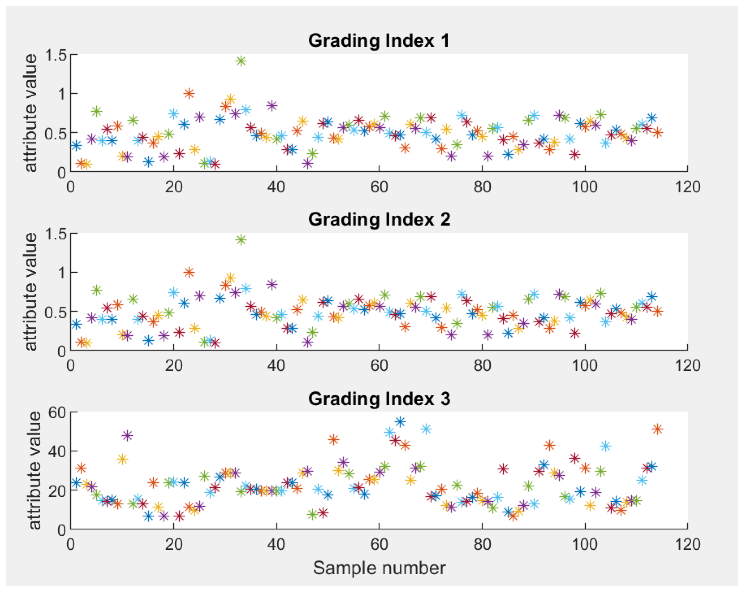
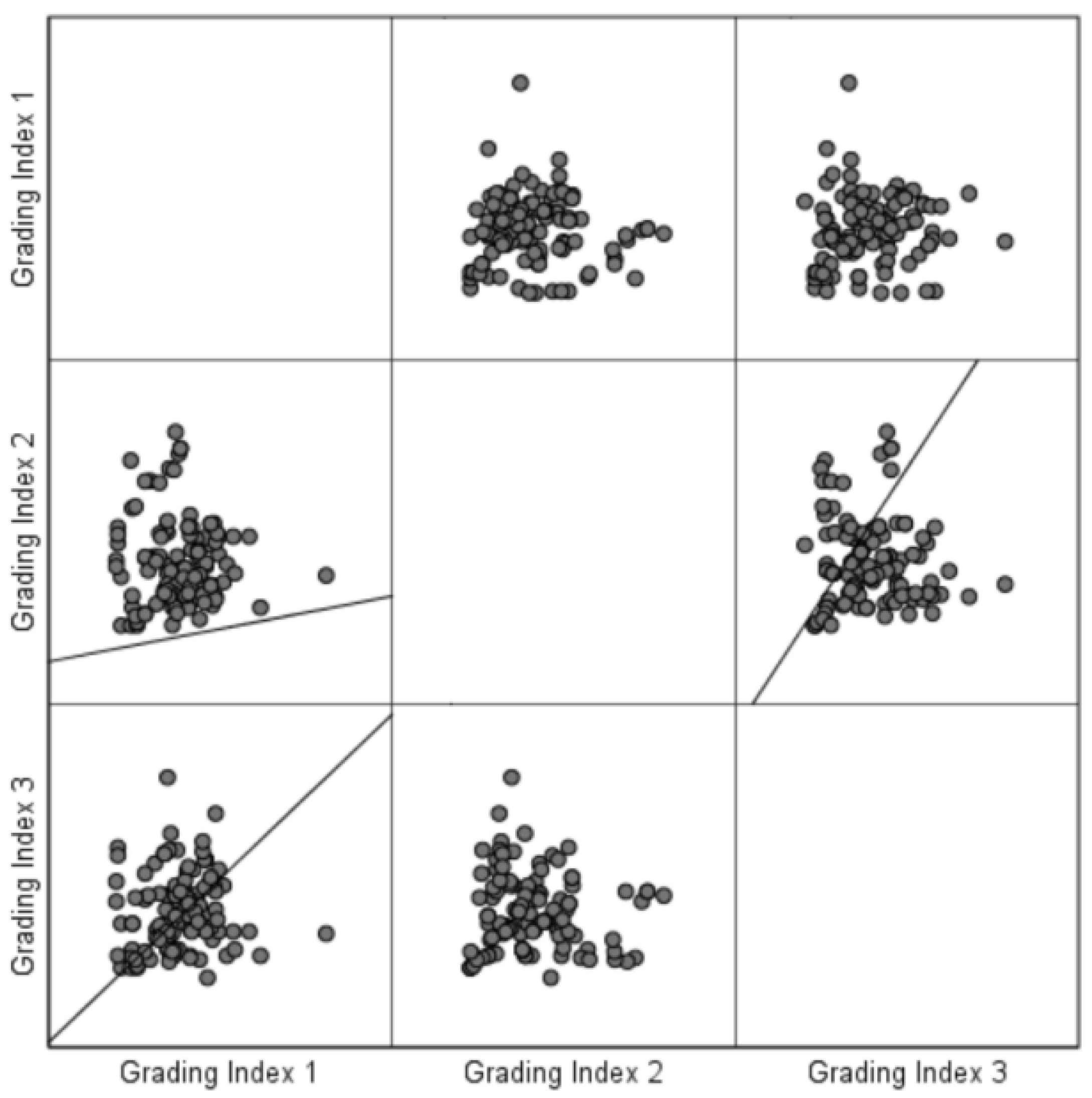
It can be seen from Figure 3 and Figure 4 that the classification index data are independent and have a relatively stable variation trend, and the error is within an acceptable range, meeting the requirements of Articles 2 and 3. Therefore, Spearman’s correlation coefficient can be used for hypothesis testing.

Table 6. Analysis results of Spearman’s index for grading indicators.

			Grading Index 1	Grading Index 2	Grading Index 3
Spearman’s Rho	Grading Index 1	correlation coefficient	1	0.039 **	0.135
		Sig.	0	0.678	0.151
		Number	114	114	114
	Grading Index 2	correlation coefficient	0.039 **	1	−0.033 ***
		Sig.	0.678	0	0.729
		Number	114	114	114
	Grading Index 3	correlation coefficient	0.135	−0.033 ***	1
		Sig.	0.151	0.729	0
		Number	114	114	114

***, p < 0.01 means rejecting the null hypothesis at the 99% confidence level. **, p < 0.05 means rejecting the null hypothesis at the 95% confidence level.

shows the Analysis Results of Spearman’s Index for grading Indicators. The null hypothesis $H_0:r=0\mathrm{and}\mathrm{the}\mathrm{alternative}\mathrm{hypothesis}{H}_1:r\ne 0$ were established to test whether the correlation coefficient was significantly different from 0. The analysis results are shown in Table 4, where rejecting the null hypothesis means that the correlation coefficient is quite different from 0. As a result, classification index 1 and the grading index correlation are substantially different from those of classification index 3 and classification index 2, respectively, with hierarchical index grade indices for 1 and 3 not being significantly different from zero. Still, the correlation coefficient is below 0.01, therefore the differences between the three classification indexes show that selection of indicators and learning samples have an excellent representative and accuracy.

In summary, the analysis of the above two methods shows that there is a high degree of difference between the three indicators based on the index analysis results of 114 groups of learning sample data, indicating that the selected indicators and learning samples have good representativeness and accuracy. The SVM hierarchical prediction discriminant model has good accuracy and persuasiveness.

4. Optimizable Support Vector Machine Model for Rock burst Intensity

4.1. Optimized Support Vector Machine Discriminant Analysis

The main idea of the SVM discriminant analysis method is based on the existing rock burst sample data, mining the internal relationship between the evaluation index and rock burst intensity, and establishing a discriminant model for judging new samples. Due to the mature application of this method in other engineering predictions, relevant contents can be referred to in [9,10,11].

4.2. Establishment and Verification of the Discriminant Analysis Model of the Optimized Support Vector Machine

According to the SVM discriminant analysis model, three rock burst intensity prediction indexes were taken as input units, 114 groups of rock burst samples were formed into learning sample sets, and four kinds of rock burst grades were taken as different output units. The SVM discriminant analysis method for rock burst intensity classification prediction proposed in this paper was trained, verified and predicted. Through the realization of the algorithm, various parameters of the optimized SVM discriminant analysis model are obtained and the results are shown in

Table 7. Training results of optimized SVM model parameters.

Training Results	Accuracy (Validation)	95.6%
	Total cost (Validation)	5
	Prediction speed	~6800 obs/s
	Training time	39.308 s
Test Results	Accuracy (Test)	100.0%
	Total cost (Test)	0
Model Type	Preset	Bayesian optimization

.

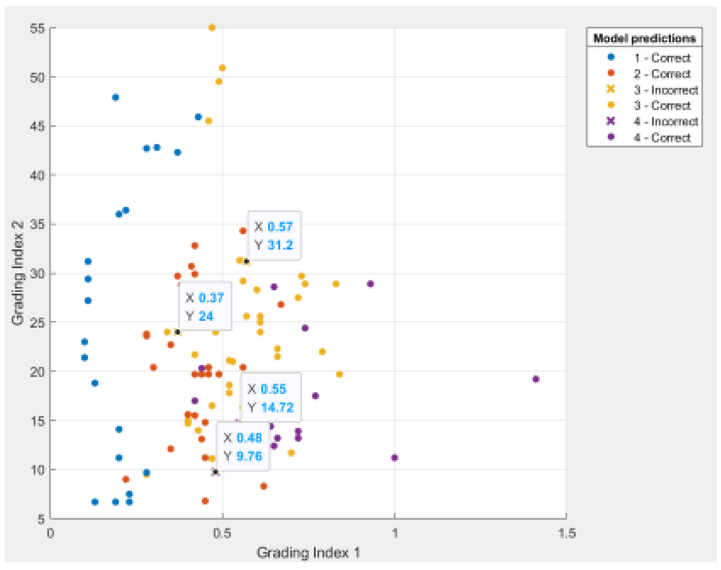
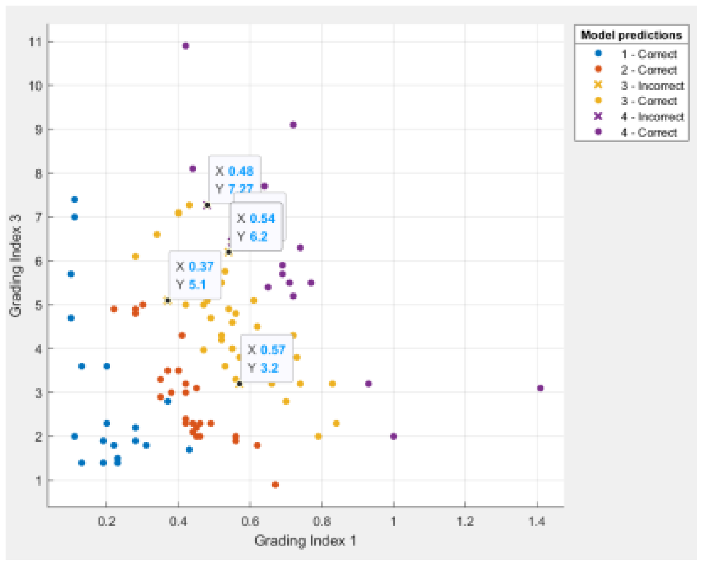
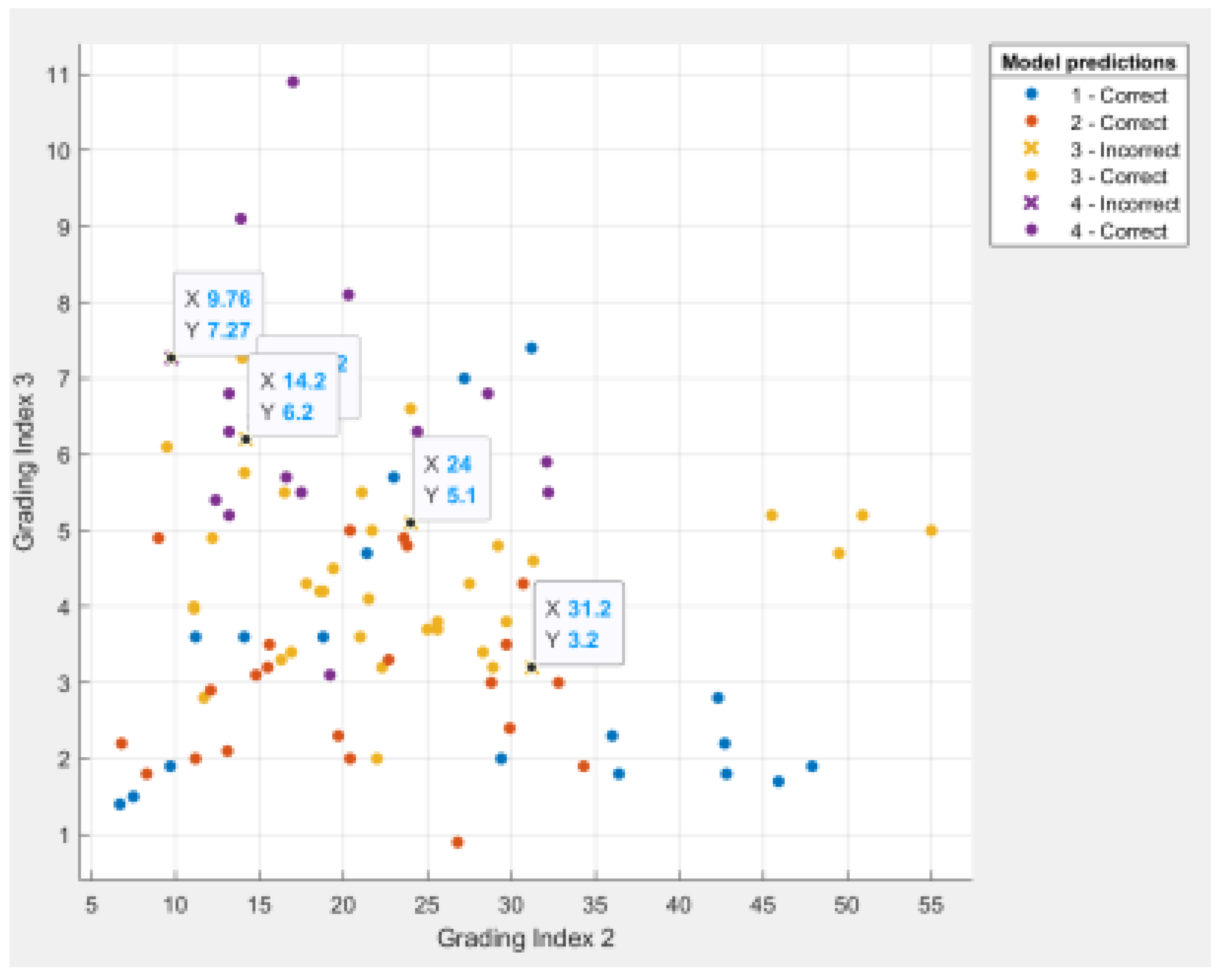
Figure 5, Figure 6 and Figure 7 show the data distribution among the three hierarchical indexes of each sample point, which can show the detailed data of the misclassified points.

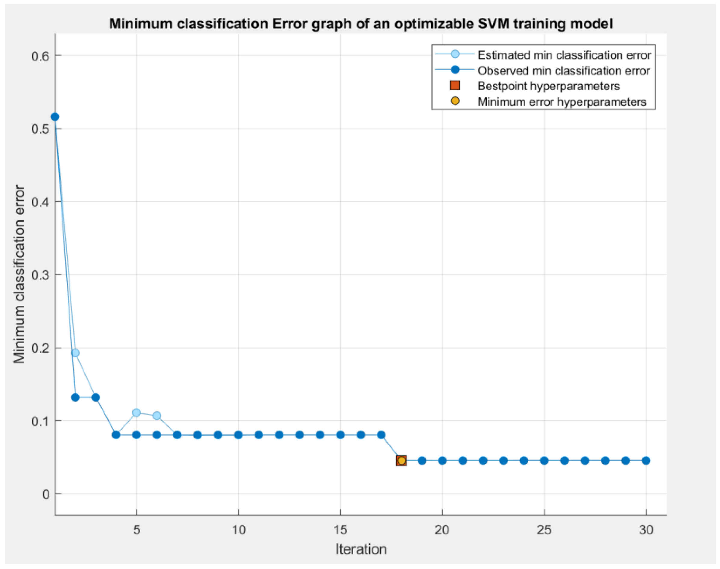
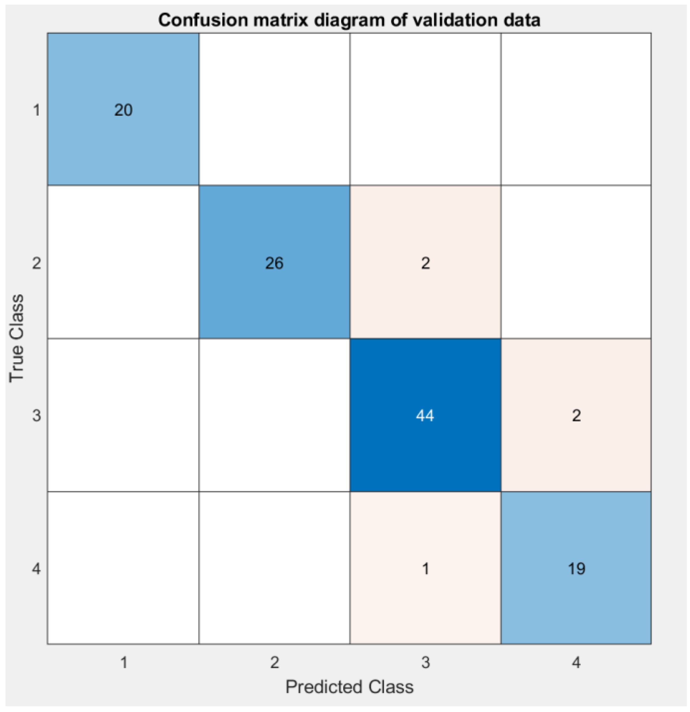
Figure 8 is the Minimum Classification Error diagram, which shows how the Minimum classification error value changes during the training process. Figure 9 shows the Confusion matrix diagram of Validation data, which shows the classification efficiency and success rate of the paper’s method.

As seen from the above-illustrated results, the discriminant results of samples numbered 7, 16, 100, 107 and 110 are inconsistent with the actual situation. The first three are misjudged as type III rock bursts (in the actual results, type III rock bursts account for 40% of the total number), and the overall misjudgment rate is only 4.38%. The discriminant error can be eliminated gradually by increasing the number of learning samples and strengthening model training. In addition, the cross-validation method is considered in this paper for model testing. Test results are used as performance indicators for the classifier or model. The goal is to achieve high predictive accuracy and low predictive error. To ensure the accuracy and stability of the cross-validation results, it is necessary to divide a test data set into different complementary subsets multiple times and cross-validate repeatedly. Take the average value of numerous validations as the validation result. The cross-validation method makes each sample data to be used as training and test data, which can effectively avoid the occurrence of over-learning and under-learning states. Through actual measurement, it is found that the accuracy of the validation data obtained by using the cross-validation method is 95.6% higher than that of the model tested by using the set-aside method, which is 92.9%. Among them, the proportion of the training set and the test set of the set-aside method is 75%:25%, and the results of the reserved method change slightly after the model is run, so it is difficult to avoid the instability of the single use of the mysterious method, which not only wastes data, but is also susceptible to overfitting, and the model correction method is not convenient. Therefore, the results obtained using the cross-validation method for model verification are accurate and persuasive.

5. Application of Engineering Examples

The trained distance discriminant model is used to classify and predict the rock burst intensity of 10 projects, respectively. The three prediction index data of samples are from the 1–1 section of the diversion tunnel of Jinping Ii Power Station [11], level 255 m of the Tongkang Mine of the China Tin Group [12], Jinchuan Ii Ore circle, Daxiangling Tunnel YK61 + 305 [13], Dongguashan Copper Mine [14] and other domestic and foreign projects [15]. Table 6 shows that the classification prediction results of the SVM discriminant model of rock burst intensity established in this paper are entirely in agreement the actual situation and have significant accuracy with the prediction results of other prediction models [15].

Table 8. Rock burst instance data and classification prediction results.

Sample Number	Classification Index			A L	Optimization of SVM P L	XGBoot Model P L	RF Model P L	SVM Model P L
	$\raisebox{1ex}{${\mathit{\sigma }}_{\mathit{\theta }}$}\!\left/ \!\raisebox{-1ex}{${\mathit{\sigma }}_{\mathit{c}}$}\right.$	$\raisebox{1ex}{${\mathit{\sigma }}_{\mathit{c}}$}\!\left/ \!\raisebox{-1ex}{${\mathit{\sigma }}_{\mathit{t}}$}\right.$	${\mathit{W}}_{\mathit{e}\mathit{t}}$
1	0.62	20	3.1	M	M	H *	M	M
2	0.61	17.9	5.3	M	M	M	M	M
3	0.44	13.1	2.1	L	L	M *	M *	L
4	0.71	32.2	5.5	H	H	H	H	H
5	0.47	11	4	M	M	H *	M	H *
6	0.25	20.77	3.80	N	N	N	L *	N
7	0.15	20.77	3.80	N	N	N	N	N
8	0.58	13.20	6.30	H	H	H	H	H
9	0.45	17.50	5.10	M	M	M	H *	H *
10	0.66	13.20	6.80	H	H	H	H	H
Precision rate					100%	70%	70%	80%

Note: A L: Actual level; P L: Predicting level. The intensity level marked * does not match the actual level.

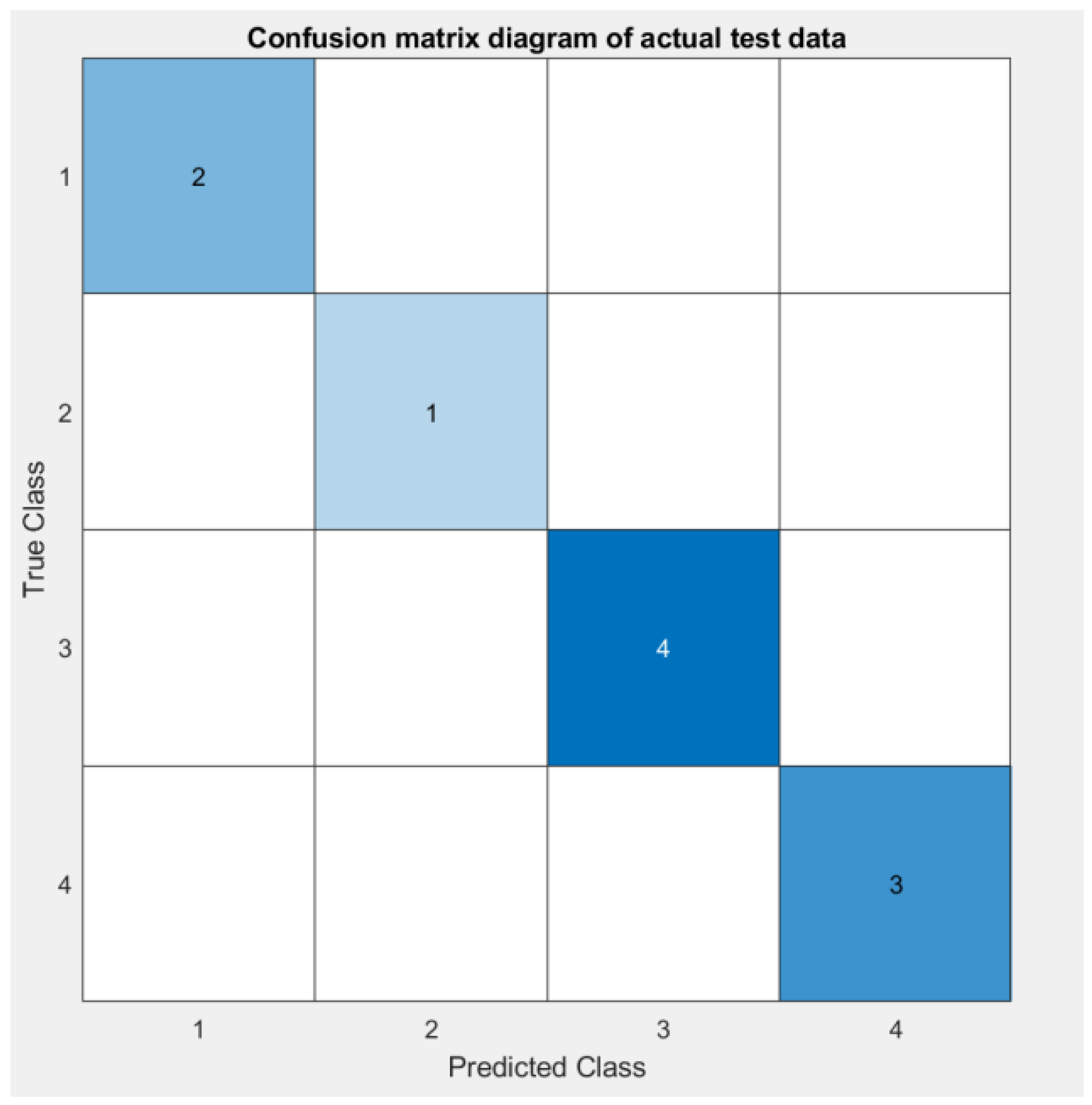
shows Rock Burst Instance data and Classification Prediction results. The accuracy of Optimization of SVM is 100% for ten samples randomly selected from different countries and different geology, which is obviously better than other representative methods. Figure 10 shows the Confusion matrix diagram of actual test data, Figure 11 shows TPR and FNR Predicted Results of Actual test data, The two graphs together show that all ten random sample points were successfully and accurately predicted.

Compared with other mathematical model methods, the SVM discriminant model does not need to consider various human factors, such as index membership degree and weight coefficient, it has high learning efficiency, and it is easy to use. It only needs to substitute the data of the samples to be predicted into the discriminant model. It can be seen that the SVM discriminant model for rock burst intensity classification prediction established in this paper based on extensive sample data has high accuracy and practicability, which can well meet the needs of engineering and can be popularized and applied.

6. Conclusions

(1)

A total of 114 groups of rock burst samples are selected, and the analysis of variance and Spearman’s correlation coefficient hypothesis test shows that the correlation between the selected three indicators is weak and has good representativeness.

(2)

The algorithm model is established based on rock burst in all kinds of data at home and abroad; therefore, the sample data are suitable for all kinds of geological conditions of rock burst prediction. In practical engineering applications, the random selection is different from the original sample data, in the case of forecasting the different geological conditions of rock burst prediction data at home and abroad. The accuracy of the final prediction results and the actual results reaches 100.00%, which shows that the algorithm is suitable for rock burst prediction under various geological conditions and has a certain adaptability.

(3)

The judgment accuracy of the optimized SVM discriminating model established was 95.6%. In the future, it is necessary to extensively collect many representative rock burst case data, expand and perfect the training sample database, and continuously improve the classification prediction accuracy.

(4)

The optimizable support vector machine (SVM) model, as a supervised learning algorithm, greatly eliminates the influence of the choice of penalty factor and kernel function on the classification performance of the SVM. The SVM algorithm can be optimized in the process of training; the advantage is that the limit parameters must be stipulated in advance, instead of in the process of model forecast adjustments, according to the classification of the real-time condition, as well as in the process of iteration for super parameters in the process of training class method, box constraint level, kernel function, the nuclear scale, and standardized data optimization adjustment, until the best classification effect is obtained.

(5)

The optimizable support vector machine model selected in this paper breaks through the experience and randomness of setting the hyperparameters of the model, and the hyperparameter optimization based on Bayesian optimization makes the accuracy of the support vector machine model reach 95.6% and 100.00% in both the learning and the actual parts. Future research can be improved by further integrating the actual situation. According to different geological conditions, the establishment and prediction of data sets can be limited to one geological situation, and then combined with the optimized support vector machine model selected in this paper for prediction, and more accurate prediction results can be obtained.

References

- Feng, X.-T. Research on Rockburst Breeding Mechanism, Early Warning and Dynamic Control Method; Wuhan Institute of Rock and Soil Mechanics, Chinese Academy of Sciences: Wuhan, China, 2012. [Google Scholar]
- Feng, X.-T. Rockburst: Mechanisms, Monitoring, Warning, and Mitigation; Elsevier: Amsterdam, The Netherlands, 2017. [Google Scholar]
- Chinanews. Yunnan Channel. A Summary of Recent Tunnel Collapses [EB/OL]. Available online: http://www.yn.chinanew.cial/2014/0916/20967.html (accessed on 16 September 2014).
- Li, P.; Chen, B.; Zhou, Y. Research progress of rockburst prediction and early warning in hard rock underground engineering. J. China Coal Soc. 2019, 44, 447–465. [Google Scholar]
- Liu, X.; Ji, H. Research on Rockburst Prediction Based on AdaBoost-BAS-SVM Model. Metal Mine 2021, 10, 28–34. [Google Scholar] [CrossRef]
- Shahriari, B.; Swersky, K.; Wang, Z.; Adams, R.P.; de Freitas, N. Taking the Human Out of the Loop: A Review of Bayesian Optimization. Proc. IEEE 2016, 104, 148–175. [Google Scholar] [CrossRef]
- Wang, Y.; Li, W.; Lee, P.K.K.; Tsui, Y.; Tham, L.G. Method of fuzzy comprehensive evaluations for rockburst prediction. Chin. J. Rock Mech. Eng. 1998, 5, 15–23. Available online: https://kns.cnki.net/kcms/detail/detail.aspx?FileName=YSLX805.002&DbName=CJFQ1998 (accessed on 1 August 2022).
- Wang, C.; Li, Y.; Zhang, C. Prediction Model of Rockburst Intensity Classification Based on Data Mining Analysis with Large Samples. J. Kunming Univ. Sci. Technol. Nat. Sci. 2020, 45, 26–31. [Google Scholar] [CrossRef]
- Wang, H.; Lu, Z.; Qiu, J.; Liu, W.; Zhang, L. Prediction of Rock Burst by Improved Particle Swam Optimization based Support Vector Machine. Chin. J. Undergr. Space Eng. 2017, 13, 364–369. [Google Scholar]
- Xu, R.; Hou, K.; Wang, X.; Liu, X.-Q.; Li, X.-B. Combined Prediction Model of Rockburst Intensity Based on Kemel Principal Component Analysis and SVM. Gold Sci. Technol. 2020, 28, 575–584. [Google Scholar]
- Zhou, J.; Li, X.B.; Shi, X.Z. Long-term prediction model of rockburst in underground openings using heuristic algorithms and support vector machines. Saf. Sci. 2012, 50, 629–644. [Google Scholar] [CrossRef]
- Zhou, K.; Lei, T.; Hu, J. RS-Topsis model of rockburst prediction in deep metal mines and its application. Chin. J. Rock Mech. Eng. 2013, 32, 3705–3711. [Google Scholar]
- Yi, Y.; Cao, P.; Pu, C. Multi-factorial Comprehensive Estimation for Jinchuan’s Deep Typical Rockburst Tendency. Sci. Technol. Rev. 2010, 28, 76–80. [Google Scholar]
- Zhang, J. Study on Prediction by Stages and Control Technology of Rock Bursthazard of Daxiangling Highway Tunnel. Ph.D. Thesis, Southwest Jiaotong University, Chengdu, China, 2010. Available online: https://kns.cnki.net/kcms/detail/detail.aspx?FileName=2010122032.nh&DbName=CMFD2010 (accessed on 1 August 2022).
- Xie, X.; Li, D.; Kong, L.; Ye, Y.; Gao, S. Rockburst propensity prediction model based on CRITIC-XGB algorithm. Chin. J. Rock Mech. Eng. 2020, 39, 1975–1982. [Google Scholar] [CrossRef]
Figure 1.
Variance relation diagram of hierarchical prediction indicators.
Figure 2.
Q–Q (Quantile) graph of classification index data.
Figure 3.
Fractal dimension visualization of grading indicators.
Figure 4.
The relationship and trend of changes among hierarchical prediction indexes.
Figure 5.
Scatter diagram of prediction results in low dimension (1).
Figure 6.
Scatter diagram of prediction results in low dimension (2).
Figure 7.
Scatter diagram of prediction results in low dimension (3).
Figure 8.
Minimum classification error diagram.
Figure 9.
Confusion matrix diagram of validation data.
Figure 10.
Confusion matrix diagram of actual test data.
Figure 11.
TPR and FNR predicted results of actual test data.