Abstract
The target of an unmanned aerial vehicle swarm will present near-field characteristics when it is integrated as an array, and the existence of the unmanned aerial vehicle swarm motion error will greatly deteriorate the beam pattern formed by the array. To solve these problems, a near-field array beamforming model with array element position error is constructed, and the Taylor expansion of the phase difference function is used to approximately simplify the model. The improved Newton maximum entropy algorithm is proposed to estimate and compensate for the phase errors. The maximum entropy objective function is established, and the Newton iterative algorithm is used to estimate the phase error iteratively. To select the proper Newton iteration initial value, based on a single reference source signal, the initial value of the phase error is estimated through the phase gradient information of the received array signal. Beamforming is carried out after phase error compensation regarding the array. In order to assess the mismatch of the phase error compensation function based on the proposed method, when the beam is scanning, the effectively compensated spatial area of the array beamforming is divided, which lays a foundation for subsequent spatial region division and unmanned aerial vehicle swarm path planning. The simulation results show that the beam formed by the method proposed in this paper has a lower sidelobe level, and as the signal-to-noise ratio changes, the robustness of the proposed method is better validated. The proposed algorithm can effectively suppress the adverse influence of array element position error on array beamforming, and when the beam is scanning, the effectively compensated area of the phase error compensation function is divided, based on the proposed method.
Keywords:
unmanned aerial vehicle swarm; antenna array; near-field beamforming; array element position error compensation; spatial area division MSC:
94-08
1. Introduction
With the development of beamforming technology and unmanned aerial vehicle swarm (UAVs) technology, the antenna array elements equipping the UAVs are combined into a distributed beamforming system through collaboration among the swarm to achieve directional high gain signal transmission. Therefore, using beamforming technology to improve the combat capability of UAVs in a fierce confrontation environment is a growing trend [1]. It is obvious that taking UAVs as an array has many advantages, such as using low-cost UAVs to achieve high gain signal transmission, which is also known as the beam pattern, but the targets of the array are often located in the near-field, and the motion error [2,3,4,5] of a single UAV as an array element will deteriorate the beam pattern formed by the array. At present, the array position error calibration is mainly founded on the calibration method of three or more known radiant sources, based on far-field signals, or the rotating array calibration method, based on a single known as a radiant source [6,7,8], but the latter is, in essence, also a multi-radiant source calibration method exchanging time for space. Reference [2] proposes using three simultaneously existing auxiliary sources to calibrate the position error of the array, but this method can only use the Taylor first-order expansion of the array steering vector with error when the position error has a very small disturbance, which means the position error cannot be corrected by this method when it is too large. In array beamforming, the beam cannot be formed when an array element position error exists, but as long as the phase error caused by the position error is compensated for, the beam can be formed effectively. It is easier to solve a one-dimensional phase error than to solve two- or three- dimensional position errors, and the phase error can be obtained by using a single known radiant source as a reference source [9,10,11,12]. As for the solution to phase error, based on the information of the reference source, the phase error can be estimated using the phase gradient (PG) value of the received signal between the array elements [13,14,15,16,17], but this method requires a high signal-to-noise ratio (SNR), and under the condition of low SNR, the deviation of the phase error estimation value from the real value is large. Phase error can also be solved by iteration. The authors of [18,19,20,21] take the entropy of the image as the objective function and estimate the phase error by using the Newton iterative method, but this method presents problems, such as the selection of the initial value affecting the algorithm time, causing the algorithm to fall into local optimization. When the expected main-lobe direction of beamforming is the same as the reference source direction, the phase error in main-lobe direction can be compensated for by the estimated phase error compensation function, but when it is not the same as the reference source direction, the mismatch of the phase error compensation function occurs, which will affect the beamforming pattern. Therefore, it is necessary to study the influence of phase error compensation function mismatch, which is the same as the division of the area effectively compensated by the estimated phase error compensation function. The authors of [22] propose that when the near-field radial compensation filter is used to filter out interference sources, the beamforming pattern will deteriorate when the sources are far away from the array, but the study does not specifically analyze the pattern deterioration level. The work in [23] proposes a method to form a multi-focus antenna array in the near-field, with specified amplitude and phase conditions for the multi-focus problem of the near-field array, but this study does not involve the analysis of the mismatch of the single-focus filter.
Based on the above analysis, firstly, a near-field array beamforming model with UAV position error is constructed in Section 2, and the model is approximately simplified by the Taylor expansion of the phase difference function of the near-field signal. Secondly, the improved Newton maximum entropy (IN-ME) algorithm is used to estimate and correct the phase error in Section 3. Under the condition of low SNR, taking the single known radiant source as a reference source, the initial value of the phase error is estimated through the PG information of the received array signal, and then, taking the maximum entropy function of the array synthetic power at the reference source as the objective function, the Newton iterative solution to the phase error is carried out. After the phase error is compensated, beamforming is carried out. Thirdly, when phase error estimation based on proposed IN-ME algorithm is used to compensate for beamforming, if the array forms beam scanning, the phase compensation function will be mismatched. Based on the phase error compensation function of the IN-ME algorithm, the effectively compensated area which can be compensated for to effectively form the beam pattern is further divided in Section 4, laying a foundation for the subsequent spatial region division and UAV path planning. The simulation results in Section 5 show the effectiveness of the algorithm, and the conclusions are given in Section 6. The adverse influence of UAV position errors on near-field array beamforming is effectively suppressed, and the effectively compensated area, with phase compensation function mismatch, is divided.
2. Near-Field Beamforming Model
2.1. Array Signal Model
Under the condition of targets being in the near-field, the assumption that the electromagnetic wave is the plane wave is not tenable, and it should be modeled as a spherical wave. As shown in Figure 1, it is assumed that the near-field antenna array of N UAVs which can be seen as N elements is linearly distributed along the axis x at equal intervals, the total length of the array is L, the coordinate of the nth element is , where, , and , refers to the distance from the nth antenna array element to the source P, R refers to the distance from the source P to the array center O, is the included angle between OP and the axis y, and when the direction of OP projection on the x axis is the same as positive direction of the x axis, is positive, and vice versa. The coordinate of source P is .
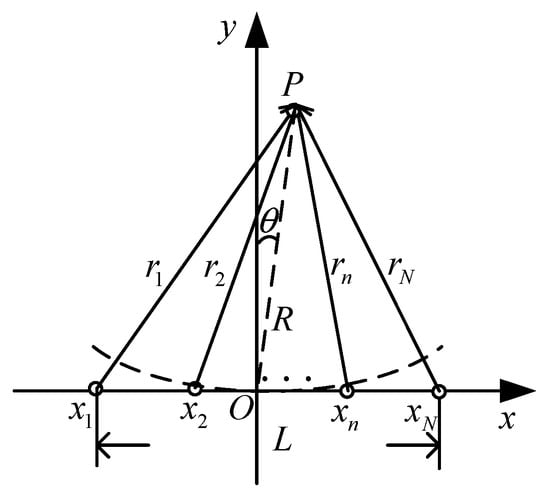
Figure 1.
Near-field array model.
For any radiant source P in the near-field, according to the spherical wave theory, the radiant signal received by the array element can be expressed as
where, is the radiant signal of the source P, j is the imaginary unit, f is the radiant signal frequency, is the wavelength, is the wavenumber, and is the wave path difference from the source P to the nth antenna array element, with the array center O as the reference point.
Theorem 1.
([24]) Suppose that is a differentiable function for which all exist, and there is neighborhood of
, in which the function value of at
can be written as .
Theorem 1 is also known as Taylor’s theorem. For the antenna array composed of UAVs, although the targets of interest in wireless communication, electronic reconnaissance, and jamming are generally located in the near-field of the array, the distances from the targets of interest to the antenna center are usually much greater than the aperture of the antenna. Therefore, it can be assumed that . Then, the Taylor series expansion of can be obtained by
Through Equation (2), the phase difference between the received signal of the nth array element and the received signal at the array center O is
By substituting Equation (3) into Equation (1) and ignoring the influence of distance on signal amplitude, the received signal model of the nth array element in the near-field can be approximately written as
For M radiant sources in the near-field, the radiant signal amplitude of the radiant source is , the frequency is , the polar coordinate is , and the distance from the nth array element to the mth radiant source is , where, . Then, the received signal of the array is
where,,, is a dimensional receiving data vector, is a dimensional array steering vector, is a dimensional signal vector, and is a dimensional noise vector. There is
where, represents matrix transpose, and the dimensional vector is the steering vector of the array under the mth radiant source.
The received signals of each array element are weighted and summed to obtain the array output as, which is beamforming
where, represents the conjugate transpose of the matrix, and is the dimensional weighted vector of the array. When the polar coordinate of the expected signal is , and the distance from the nth array element is , there is , where, .
2.2. Actual Near-Field Beamforming
When there are errors in the positions of the array elements, the actual coordinate of the nth array element is , where, , and . Under the model of this paper, . Similar to 2.1., the modified actual wave path difference in the Taylor series expansion is
By using Equation (10) to approximately simplify , the actual nth array signal model can be expressed as
Then the actual received signal of the array is
where, is an actual dimensional received data vector, is the actual is the received radiant source signal, is an actual dimensional array steering vector, and
where, is the error value of the nth array element. When , the actual beamforming formula can be written as
where, is the conjugate complex of .
Obviously, due to the presence of array position errors and noises, it is impossible to effectively carry out near-field beamforming by using the signal weight that can be obtained when the array is at the nominal value to compensate for the actual signal.
3. IN-ME Phase Error Compensation Algorithm Based on Reference Source
Only by compensating for phase error can the array effectively form a beam pattern. We propose the IN-ME algorithm, which, compared to Newton maximum entropy (N-ME) algorithm, can obtain higher convergent value within a shorter period, as well as form a lower sidelobe-level beam pattern with a higher SNR.
3.1. Phase Error Estimation Based on Newton Maximum Entropy Algorithm
Entropy is a measurement of information uncertainty. The maximum entropy principle is a criterion of probabilistic model learning, and when the probability distribution of random variables obeys uniform distribution, the entropy reaches its highest level. As for beamforming, we expect that after phase error compensation, the synthetic powers in the main-lobe direction of the array’s received signals in all snapshots increase, which becomes a multi-objective optimization problem. If we regard the ratio of synthetic power in the main-lobe direction of the array’s received signals in one snapshot to the sum of the synthetic powers in all snapshots as the probability distribution, compared to the maximum entropy principle, it can be seen as that when this ratio obeys uniform distribution, the synthetic power in every snapshot can increase, which means that the phase error compensation is effective for the signals in every snapshot. Therefore, the objective function should be the maximum entropy of that ratio.
Assuming that there is a reference source in the target scene, if the array beamforming is expected to form a main-lobe at the source, the weighted value of the array can be obtained as . When the snapshots are certain, , representing the total ideal synthetic power of all snapshots at the reference point, is a constant, and can be obtained by
where, SS is the total number of snapshots, and is the synthesized signal at the reference source after ideally weighting and summing the received signals in the ssth snapshot. The synthetic power in the main-lobe direction of the array’s received signals in one snapshot can be obtained by
where, is the received signal in the ssth snapshot of the array element, and is the phase error of the nth array element to be estimated. Because is a constant, the entropy objective function of can be written as
The entropy objective function is the function of the phase to be estimated. Thus, the phase estimation based on the maximum entropy can be expressed as
Theorem 2.
([25]) Suppose that , which is the second derivation of ,
is continuous in an open neighborhood of , and that and is negative definite. Then is a strict local maximizer of .
Proof.
Because , which is also known as the Hessian, is a continuous and negative definite at , we can choose a radius so that remains negative definite for all x in the open ball . Taking any nonzero vector with , we have , and so , where, for some . Since , we have , and therefore , giving the results. □
By combining Theorem 1 and Theorem 2, we can use the Newton method for Formula (20). There is an iterative solution of as
where, superscript indicates the lth iteration. To solve Equation (21), the first and second derivation of against need to be calculated. The first derivative expression can be expressed as
The second derivative expression can be expressed as
where,
where, represents the real part operation.
In practical cases, the phase errors in signals received by different array elements are relatively independent from each other [26]. Therefore, the phase error of each array element is searched separately, and in Formula (23), only the diagonal elements of the Hessian, which is also the second derivative , of the entropy with respect to phase error are derived, while the off-diagonal elements are ignored.
By taking Equations (24) and (25) into Equation (22), the analytical formula of the first derivative is obtained
By taking Equation (24) to Equation (28) into Equation (23), the analytical formula of the first derivative is obtained
After performing phase error calibration for Equation (16), the beamforming with error calibration is
where, represents the Hadamard product of the matrix, and .
3.2. Initial Value Estimation of Phase Error Based on PG
According to the principle of Newton’s maximum entropy algorithm, the selection of the initial value of the phase error will directly affect the iteration efficiency. If the initial value of the phase error is randomly selected, such as directly setting the initial value of phase error to zero, which is the N-ME algorithm, it may not only greatly slow down the convergence speed of the algorithm, but also make the algorithm fall into the local optimal solution. Therefore, a method based on a reference source to select the initial value of the phase error is proposed to improve the N-ME algorithm.
When there are noises and array position errors, after weighting the received signals, the initial received signals of the array without phase error calibration can be written as
where, represents conjugation, represents the initial output signal of the nth array element, and represents the initial phase error of the nth array element caused by noise and array position error.
Ideally, after weighting the received signals, the phase error caused by different distances is fully compensated, and the PG between the output signals of the array elements is constant. For discrete sequences, the phase difference between the output signals of adjacent array elements is the PG. We define the correlation sequence of the array as
The PG between adjacent elements is estimated as
By taking the phase of the first array element as a reference, the initial value of phase error to be compensated for each array element is estimated by calculating the cumulative sum between adjacent array elements. There is
where, represents the cumulative sum.
The IN-ME phase error compensation algorithm, based on the reference source, is shown in Algorithm 1.
| Algorithm 1 The IN-ME phase error compensation algorithm based on reference source. |
| >Input: received signals of array , reference source Output: beamform after phase error calibration Step 1: Calculate weighted signal, weights , and weighted signal ; Step 2: Calculate the correlation sequence of the array, ; Step 3: Estimate initial value of phase error based on PG: 1. Estimate the PG between adjacent elements, ; 2. Estimate initial value of phase error, ; Step 4: Improved Newton Maximum Entropy Algorithm: 1. Calculate the array’s synthetic signal at the reference source, ; 2. Form the entropy objective function, ; 3. Calculate the first and second derivatives of to , , ; 4. Use Newton iterative method for optimization, ; Step 5: Beamform after error calibration, . |
4. Effectively Compensated Area
The phase error compensation based on phase error compensation function of the IN-ME algorithm is aimed at the situation in which the expected main-lobe of beamforming is just at the reference source . When the expected main-lobe of beamforming is not at the reference source, there is a mismatch between the phase error compensation function and the actual phase error. Thus, it is necessary to discuss the effectively compensated area based on the phase error compensation function of the IN-ME algorithm.
Assuming that the position errors of the array elements are independent of each other and meet the normal distribution with the mean value of 0 and the variance of , which is, for the nth UAV element, and , and the two-dimensional joint distribution of the two also meets the normal distribution, according to the “ rule”, the elements can be regarded approximately as that they are located in a circle with the radius centered on the ideal array element position, as shown in Figure 2. When the expected main-lobe of beamforming is at the source , but the reference source of the IN-ME algorithm is , the effectively compensated area based on the phase error compensation function of the IN-ME algorithm can be approximately solved by geometric methods.
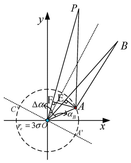
Figure 2.
Geometric relation between the array elements, with position error and radiant source.
Obviously, when the actual position of the array element is on the circle, the phase error is larger than when it is in the circle. Point A is set as a moving point on the circle to represent the actual position of the nth array element. When the two sources, and , have relative phase errors , it is considered that the compensation is effective [27,28]. There is
where, and are respectively the axis and axis coordinates of point A.
As shown in Figure 2, crossing point A, the plumb line AF, which is perpendicular to PO, is made, and the point of intersection is point F. The plumb line AE, which is perpendicular to BO, is made, and the point of intersection is point E. We let , , and . When and , the electromagnetic wave from or to any point on the circle can be approximately simplified to the plane wave, and we have and . Then Equation (36) is approximately simplified as
By using sum-to-product addition formulas, there is . Then there is
As shown in Figure 2, the perpendicular line of the angular bisector which is made through the center O of the circle intersects with the circle at and . Equation (38) shows that the expected point A which can get max(fit) approximately locates at or , according to
The area of that can be compensated based on for the nth array element can be obtained by
After finding out the upper and lower bounds of the area of the phase error for each array element can be effectively compensated, and the area can be divided by finding the intersection of the area of all array elements. As shown in Figure 3, the connecting line from the nth array element to is marked as line , which is the angular bisector of , and the line towards the negative angle direction is line , while the line towards the positive angle direction is line . The intersection point of line and line is marked as point . The intersection point of line and line is marked as point . The line parallel to line is started from point , and the connecting line between and is marked as line . The intersection point of and is marked as point , and line parallel to is started from . The connecting line between and is marked as line . Then the effectively compensated area of the array for based on is within the area encircled by four sides of g, e, d, and f.
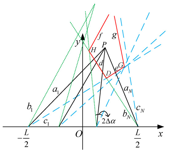
Figure 3.
The effectively compensated area of emitter .
As shown in Figure 3, the problem of finding the effectively compensated area is transformed into the problem of finding the intersection point of the lines, and the equations of the black line cluster can be expressed as
The equation of the green line cluster can be expressed as
The equation of the blue line cluster can be expressed as
Let , , and , and coordinates of H, D and G can be obtained by
The analytic expressions of the red four sides g, e, d, and f are
The area encircled by the four edges shown in Equation (45) is the effectively compensated area of that can be compensated based on IN-ME algorithm.
By estimating and compensating the phase errors, the phase errors of the received signals caused by the position of the array elements in the array are calibrated so that the antenna array of UAVs can effectively carry out beamforming. The analysis of the effectively compensated area based on the reference source can provide a reference for the target area division and path planning of UAVs.
5. Simulation Analysis
5.1. IN-ME Phase Error Compensation Algorithm Based on Reference Source
We suppose that the signal frequency , wavelength , number of array elements , array aperture , main-lobe of beam is at known radiant source , whose polar coordinates are or and , the number of signal snapshots , array element position error and are independent of each other, and they both meet the normal distribution with a mean value of 0 and a standard deviation of , and the low SNR is −3 dB. We use the N-ME algorithm, IN-ME algorithm, adaptive differential evolution algorithm (ADE) [29], and genetic algorithm (GA), respectively, to estimate the phase error; the changes in the maximum entropy of the array signal synthetic power, along with the number of iterations of the algorithms, are shown in Figure 4. The reason why we adopt ADE and GA is because they are both artificial intelligence algorithms, which are different from our algorithm and are widely used in solving multi-objective search problems and beamforming [29,30,31,32,33]. The objective function of both ADE and GA is the entropy objective function, as shown in Formula (19). The parameters of ADE are that the population number of the genetic algorithm is 100, the mutation rate is 0.5, and the crossover probability is 0.9. The parameters of GA are that the hybridization rate is 0.7, the mutation rate is 0.05, and the “roulette wheel” selection is used. The elitist retention strategy is adopted. It is worth noting that all of our simulation tests are respectively based on the average of 1000 Monte Carlo tests.
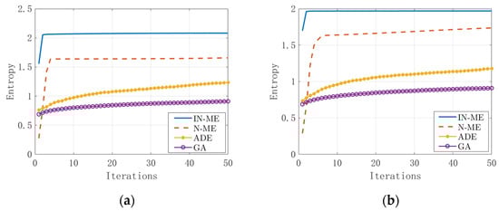
Figure 4.
Comparison of different algorithms. (a) ; (b) .
As shown in Figure 4, the convergence rates of ADE and GA are slower than those of N-ME and IN-ME, and within 50 iterations, the entropy value of ADE and GA cannot reach the same high rate as those reached by N-ME or IN-ME, which shows that ADE and GA are inferior to N-ME and IN-ME, and this is because the search direction of ADE and GA is aimless, while N-ME and IN-ME search along the gradient descent direction. Compared with IN-ME, the N-ME algorithm will require more iterations and a longer period to converge, and will easily fall into local optimization, eventually reaching a smaller entropy value. Compared with the N-ME algorithm, the IN-ME algorithm proposed in this paper makes the entropy objective function of the algorithm converge faster and reach a larger entropy value, which verifies the effectiveness of IN-ME. Because of the adverse performance of ADE and GA, N-ME and IN-ME are used to form beams and make comparisons. After phase error compensation, when , beamforming is shown in Figure 5a. When the beam is scanning and , the compensation effect is shown in Figure 5b.
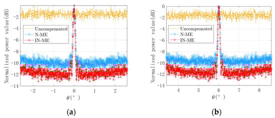
Figure 5.
Comparison of the beam forming effect after phase compensation. (a) ; (b) .
As shown in Figure 5, whether beam scans or not, beams cannot be formed because of the uncompensated phase error; the sidelobe level of the N-ME algorithm is approximately −9.5 dB, and the sidelobe level of IN-ME algorithm is approximately −12 dB, which means that the beamforming algorithm proposed in this paper can better compensate for the phase error of array elements and obtain a lower sidelobe level.
In order to compare the ideal beamforming (IB) with noise, phase gradient beamforming (PGB), the N-ME beamforming algorithm, and the IN-ME beamforming algorithm in different SNR backgrounds, by taking beamforming without scanning as an example, scenarios in which SNR changes from −12 dB to 9 dB are simulated, and the beamforming results are shown in Figure 6.
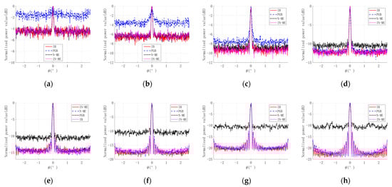
Figure 6.
Beamforming contrast of two algorithms when SNR changes. (a) SNR = −12 dB; (b) SNR = −9 dB; (c) SNR = −6 dB; (d) SNR = −3 dB; (e) SNR = 0 dB; (f) SNR = 3 dB; (g) SNR = 6 dB; (h) SNR = 9 dB.
As shown in Figure 6, with the SNR changing from −12 dB to 9 dB, both the N-ME and IN-ME algorithms can effectively form a beam pattern. When the SNR is low, using the phase error estimated by PG information to compensate the array cannot effectively form a beam pattern, but with increasing SNR, the beam formed by PG gradually improves, compared to the beam formed by the N-ME. The IN-ME beamforming algorithm proposed in this paper can continuously remain nearly the same as ideal beamforming with noise; when the SNR is low, it performs better than PGB, and when SNR is high, it performs better than the N-ME beamforming algorithm, which shows the advantages of the IN-ME algorithm.
5.2. Effectively Compensated Area
We assume that the position errors corresponding to the phase errors and are independent of each other and meet the normal distribution of 0 mean value and , which is and . According to the “ rule,” we can get , and from Equation (40). The area that can be effectively compensated by each array element is within the area whose angular bisector is the line from the known radiant source shown as red * to the ideal position of the array element, and the angular area is between , as shown in Figure 3. As shown in Figure 2, we set or , , and or . According to Equation (36) through Equation (45), the effectively compensated area and the corresponding dividing points D, H, and G are shown as red * in Figure 7.
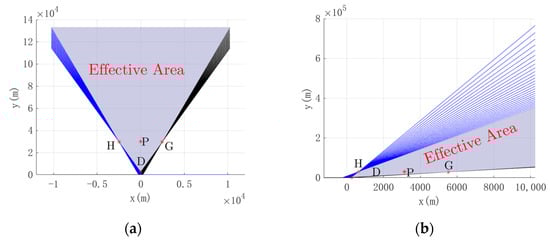
Figure 7.
Effectively compensated area. (a) ; (b) .
According to Figure 7, we see that when the radiant source is located on the vertical line in the array, the effectively compensated area is greater than when it is located at a certain angle relative to the vertical line of the array. In order to verify the effectively compensated area shown in Figure 7, taking Figure 7a as an example, let the radiant source M be a moving source, whose coordinates are and , the main-lobe is expected to point to the direction of the radiant source M, and the phase calibration function based on the IN-ME algorithm is used to compensate the beamforming. The movement track of the radiant source M is shown by the thick solid green line in Figure 8a. The power value change in the direction of the radiant source M is calculated, which is in the direction of the main-lobe, and the boundary points H, G, and of are marked, as shown in Figure 8b.
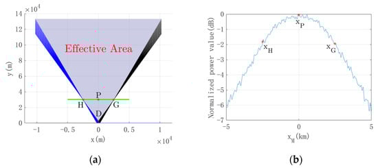
Figure 8.
Change of main-lobe power within the effectively compensated area; (a) moving radiant source trajectory; (b) variation of main-lobe power value with .
As shown in Figure 8, due to the influence of noise, when , the power value in the main-lobe direction, where the radiant source M is located, fluctuates, but changes regularly as a whole with the change of . When , the radiant source M is outside the effectively compensated area, and the power value in the main-lobe direction decreases by more than 3 dB, which shows that the compensation is invalid. When , the radiant source M is within the effectively compensated area, and the power value in the main-lobe direction drops within 3 dB, which shows that the compensation is effective. The closer is to , the greater the power value is in the main-lobe direction, which means the better the compensation is.
Similarly, the main-lobe power change within the effectively compensated area during beam scanning is simulated in Figure 9.
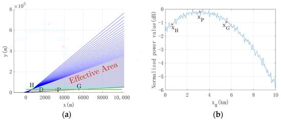
Figure 9.
Change of main-lobe power within the effectively compensated area using beam scanning; (a) moving radiant source trajectory; (b) variation of main-lobe power value with .
A conclusion similar to that in Figure 8 is obtained from Figure 9. When the radiant source M is outside the effectively compensated area, the power value in the main-lobe direction decreases by more than 1 dB, which is considered that the compensation is noneffective. When the radiant source M is within the effectively compensated area and the power value in the main-lobe direction drops within 1.5 dB, which is considered that the compensation is effective. The closer is to , the greater the power value is in the main-lobe direction, which means the better the compensation is.
All in all, as can be seen from Figure 8b and Figure 9b, the method proposed in this paper divides the area into a subset of the area with the power value in the main-lobe direction decreasing by 3 dB as a boundary value, ensuring the effectiveness of the division area for compensation. This effectively compensated area is related to the selection of the effective standard for phase compensation in Equation (36).
6. Conclusions
In order to solve the problems of UAV near-field beamforming, UAV position error compensation, and the effectively compensated area of compensation, this paper firstly constructs a near-field array beamforming model based on element position error, and approximately simplifies the model using the Taylor expansion of the near-field signal phase difference function. Moreover, an IN-ME algorithm is proposed to estimate and compensate for the phase error. Based on the known reference source signal, the initial value of the phase error is estimated through the PG information of the array’s received signal, and then the array signal entropy objective function is established to iteratively optimize the phase error value using the Newton iteration method, and the beam pattern is formed after the phase error compensation. Thirdly, when the beam scanning leads to the phase compensation function mismatch, based on the phase error compensation function of the IN-ME algorithm, the effectively compensated area is further divided, which lays a foundation for the subsequent area region division and UAV path planning. Finally, the validity of the conclusion is verified by simulation. By using the IN-ME algorithm proposed in this paper, the influence of a single UAV’s position error on array beamforming is effectively suppressed, and the effectively compensated area is divided because of phase compensation function mismatch, which provides a theoretical basis for the UAV beamforming application in wireless communication, electronic reconnaissance, and jamming. As the signal wavelength becomes shorter, the adverse influence of the UAV’s position error increases, and the beam pattern will deteriorate sharply, which is worthy of further research.
Author Contributions
Conceptualization, S.P., G.W., Y.Z., G.Y. and Y.L.; data curation, Y.Z. and G.W.; formal analysis, Y.Z. and G.W.; funding support, Y.L.; writing—original draft, Y.Z.; writing—review and editing, S.P., G.W., G.Y. and Y.L. All authors have read and agreed to the published version of the manuscript.
Funding
This research was funded by the Military Scientific and Technological Commission, and the Airforce of the People’s Liberation Army, Government of China, under grant number 21KJ3C1-0090R and PGGC-2021-003.
Institutional Review Board Statement
Not applicable.
Informed Consent Statement
Not applicable.
Data Availability Statement
Not applicable.
Conflicts of Interest
The authors declare no conflict of interest. The funders had no role in the design of the study; in the collection, analyses, or interpretation of data; in the writing of the manuscript; or in the decision to publish the results.
References
- Silvus to Develop DARPA Distributed Beamforming Technology. Available online: https://www.unmannedsystemstechnology.com/2021/03/silvus-to-develop-distributed-beamforming-technology-for-darpa/ (accessed on 19 March 2021).
- Wang, Y.L.; Chen, H.; Peng, Y.; Wan, Q. Spatial Spectrum Estimation Theory and Algorithm; Tsinghua University Press: Beijing, China, 2004; pp. 416–417. [Google Scholar]
- Shu, R.; Xu, Z. Lidar Imaging Principle and Motion Error Compensation Method; Science Press: Beijing, China, 2014; pp. 28–32. [Google Scholar]
- Feng, F.Y.P.; Rihan, M.; Huang, L. Positional Perturbations Analysis for Micro-UAV Array With Relative Position-Based Formation. IEEE Commun. Lett. 2021, 25, 2918–2922. [Google Scholar] [CrossRef]
- Umeyama, A.Y.; Salazar-Cerreno, J.L.; Fulton, C.J. UAV-Based Far-Field Antenna Pattern Measurement Method for Polarimetric Weather Radars: Simulation and Error Analysis. IEEE Access 2020, 8, 191124–191137. [Google Scholar] [CrossRef]
- Wang, D.; Zhang, P.; Yang, Z.; Wei, F.; Wang, C. A Novel Estimator for TDOA and FDOA Positioning of Multiple Disjoint Sources in the Presence of Calibration Emitters. IEEE Access 2020, 8, 1613–1643. [Google Scholar] [CrossRef]
- Ni, M.; Chen, H.; Cheng, Y.; Ni, L.; Wang, X. Sensor Position Errors Calibration Algorithm of Near-field Source Based on Fourth-order Cumulant. In Proceedings of the IEEE International Conference on Signal, Information and Data Processing, Chongqing, China, 11–13 December 2019; pp. 1–5. [Google Scholar] [CrossRef]
- Sippel, E.; Lipka, M.; Geiß, J.; Hehn, M.; Vossiek, M. In-Situ Calibration of Antenna Arrays Within Wireless Locating Systems. IEEE Trans. Antennas Propag. 2020, 68, 2832–2841. [Google Scholar] [CrossRef]
- Ahmed, M.M.; Ho, D.K.C.; Wang, G. Localization of a Moving Source by Frequency Measurements. IEEE Trans. Signal Process. 2020, 68, 4839–4854. [Google Scholar] [CrossRef]
- Shi, S.; Li, C.; Hu, J.; Zhang, X.; Fang, G. Study of Phase Error Reconstruction and Motion Compensation for Terahertz SAR With Sparsity-Promoting Parameter Estimation. IEEE Trans. Terahertz Sci. Technol. 2021, 11, 122–134. [Google Scholar] [CrossRef]
- Yang, C.; Zheng, Z.; Wang, W.-Q. Calibrating Nonuniform Linear Arrays With Model Errors Using a Source at Unknown Location. IEEE Commun. Lett. 2020, 24, 2917–2921. [Google Scholar] [CrossRef]
- Wei, T.; Liao, B.; Huang, H.; Quan, Z. Online Mutual Coupling Calibration Using a Signal Source at Unknown Location. In Proceedings of the IEEE the 10th Sensor Array and Multichannel Signal Processing Workshop, Sheffield, UK, 8–11 July 2018; pp. 189–193. [Google Scholar]
- Zhou, L.; Yu, H.; Lan, Y. Deep Convolutional Neural Network-Based Robust PG Estimation for Two-Dimensional Phase Unwrapping Using SAR Interferograms. IEEE Trans. Geosci. Remote Sens. 2020, 58, 4653–4665. [Google Scholar] [CrossRef]
- Li, Y.; O’Young, S. Kalman Filter Disciplined PG Autofocus for Stripmap SAR. IEEE Trans. Geosci. Remote Sens. 2020, 58, 6298–6308. [Google Scholar] [CrossRef]
- Li, Q.; Liu, W.; Huang, L.; Sun, W.; Zhang, P. An Undersampled Phase Retrieval Algorithm via Gradient Iteration. In Proceedings of the IEEE the 10th Sensor Array and Multichannel Signal Processing Workshop, Sheffield, UK, 8–11 July 2018; pp. 228–231. [Google Scholar]
- Zou, H.; Zhong, L.; Li, J.; Sun, Z.; Liu, Y.; Ning, Q.; Lu, X. Phase Extraction Algorithm Based on the Spatial Carrier-Frequency Phase-Shifting Gradient. IEEE Photonics J. 2019, 11, 1–7. [Google Scholar] [CrossRef]
- Kumar, B.; Kumar, A.; Bahl, R. Performance Analysis of Phase and Amplitude Gradient Method for DoA Estimation using Underwater Acoustic Vector Sensor. In Proceedings of the 2019 IEEE Underwater Technology, Kaohsiung, Taiwan, 16–19 April 2019; IEEE: Taiwan, China, 2019; pp. 1–4. [Google Scholar]
- Shi, S.; Li, C.; Fang, G.; Zhang, X. A THz SAR Autofocus Algorithm Based on Minimum-Entropy Criterion. In Proceedings of the 44th International Conference on Infrared, Millimeter, and Terahertz Waves, Paris, France, 1–6 September 2019; pp. 1–2. [Google Scholar] [CrossRef]
- Li, G.; Fang, S.; Han, B.; Zhang, Z.; Hong, W.; Wu, Y. Compensation of Phase Errors for Spotlight SAR With Discrete Azimuth Beam Steering Based on Entropy Minimization. IEEE Geosci. Remote Sens. Lett. 2021, 18, 841–845. [Google Scholar] [CrossRef]
- Li, J.; Ye, Q.; Guo, J.; Min, R.; Li, Y. Motion Compensation Algorithm Based on Entropy-Minimization for Terahertz SAR. In Proceedings of the 14th UK-Europe-China Workshop on Millimetre-Waves and Terahertz Technologies, Lancaster, UK, 13–15 September 2021; pp. 1–3. [Google Scholar]
- Zhang, S.; Liu, Y.; Li, X.; Bi, G. Joint Sparse Aperture ISAR Autofocusing and Scaling via Modified Newton Method-Based Variational Bayesian Inference. IEEE Trans. Geosci. Remote Sens. 2019, 57, 4857–4869. [Google Scholar] [CrossRef]
- Fisher, E.; Rafaely, B. Near-Field Spherical Microphone Array Processing With Radial Filtering. IEEE Trans. Audio Speech Lang. Process. 2011, 19, 256–265. [Google Scholar] [CrossRef]
- Liu, R.; Wu, K. Antenna Array for Amplitude and Phase Specified Near-Field Multifocus. IEEE Trans. Antennas Propag. 2019, 67, 3140–3150. [Google Scholar] [CrossRef]
- Spivak, M. Calculus, 3rd ed.; Perish Inc.: Houston, TX, USA, 1967; pp. 405–411. [Google Scholar]
- Nocedal, J.; Wright, S.J. Numerical Optimization; Springer: New York, NY, USA, 1999; pp. 15–18. [Google Scholar]
- Zhang, S.; Liu, Y.; Li, X. Fast Entropy Minimization Based Autofocusing Technique for ISAR Imaging. IEEE Trans. Signal Process. 2015, 63, 3425–3434. [Google Scholar] [CrossRef]
- Van Tree, H.L. Optimum Array Processing; John Wiley & Sons, Inc.: New York, NY, USA, 2002; pp. 120–126. [Google Scholar]
- Johnson, D.H.; Dudgon, D.E. Array Signal Processing: Concepts and Techniques; PTR Prentice Hall: Upper Saddle River, NJ, USA, 1993; pp. 124–182. [Google Scholar]
- Zhang, Y.N.; Yu, G.W.; Peng, S.R.; Leng, Y.; Wang, G.X. Antenna Beam Optimization for Near-field Super-sparse Array Based on UAVs. In Proceedings of the 5th International Conference on Electronic Information Technology and Computer Engineering (EITCE), Xiamen, China, 22–24 October 2021; pp. 1541–1548. [Google Scholar]
- Jiang, Z.J.; Zhao, S.; Chen, Y.; Cui, T.J. Beamforming Optimization for Time-Modulated Circular-Aperture Grid Array With DE Algorithm. IEEE Antennas Wirel. Propag. Lett. 2018, 17, 2434–2438. [Google Scholar] [CrossRef]
- Pradhan, D.; Wang, S.; Ali, S.; Yue, T.; Liaaen, M. CBGA-ES+: A Cluster-Based Genetic Algorithm with Non-Dominated Elitist Selection for Supporting Multi-Objective Test Optimization. IEEE Trans. Softw. Eng. 2021, 47, 86–107. [Google Scholar] [CrossRef]
- Dadallage, S.; Yi, C.; Cai, J. Joint Beamforming, Power, and Channel Allocation in Multiuser and Multichannel Underlay MISO Cognitive Radio Networks. IEEE Trans. Veh. Technol. 2016, 65, 3349–3359. [Google Scholar] [CrossRef]
- Souto, V.D.P.; Souza, R.D.; Uchôa-Filho, B.F.; Li, Y. A Novel Efficient Initial Access Method for 5G Millimeter Wave Communications Using Genetic Algorithm. IEEE Trans. Veh. Technol. 2019, 68, 9908–9919. [Google Scholar] [CrossRef]
Publisher’s Note: MDPI stays neutral with regard to jurisdictional claims in published maps and institutional affiliations. |
© 2022 by the authors. Licensee MDPI, Basel, Switzerland. This article is an open access article distributed under the terms and conditions of the Creative Commons Attribution (CC BY) license (https://creativecommons.org/licenses/by/4.0/).