A Novel Improved GSA-BPSO Driven PID Controller for Load Frequency Control of Multi-Source Deregulated Power System

Abstract

In this paper, a novel improved gravitational search algorithm–binary particle swarm optimization (IGSA-BPSO) driven proportional-integral-derivative (PID) controller is proposed to deal with issues of automatic generation control (AGC) of interconnected multi-source (thermal-hydro-gas) multi-area deregulated power systems. The effectiveness and robustness of the proposed controller is compared and analyzed with GSA and PSO-driven PID controllers. The simulated and mathematically formulated results show the superiority of the proposed IGSA-BPSO driven PID controller compared with the other two techniques in settling time, overshoot, and convergence time. The two-area test system considered in this article is integrated with a thermal, hydro, and gas turbine power plant. Integral time multiplied by absolute error (ITAE) is used as the objective function (minimization) by optimization techniques for getting optimum parameters of PID controllers installed in each area. The system’s dynamics are examined using poolco, bilateral, and contract violation cases under a deregulated environment, and the comparative results are shown to analyze the efficacy of the proposed concept. Physical constraints such as generation rate constraints (GRC) and time-delay (TD) have been considered in the system as a realistic approach. This paper considers an accurate AC-DC tie-link model for the proposed AGC mechanism. Dynamic load change condition is tested and verified. The variations of different parameters will be used in the robustness analysis of the proposed system. The comparison shows that the designed controllers are more robust and produce better results than those considered as references.

1. Introduction

Automatic generation control (AGC) plays a pivoted role in the operation and control of electric power systems. Frequency, generation, and tie-line power all deviate from their specified line power values due to the persistent disparity between total generation and stated power consumption. Therefore, system integrity must be maintained in real time by matching generation, load needs, and associated losses. The reliability of network operation is directly affected by frequency deviation from its nominal range. Therefore, the hasty maintenance of the planned frequency values and the cross-line power exchange with neighboring control areas are the two main goals of an AGC scheme. Our two main objectives are to maintain both the system’s frequency and tie-line power deviation within the desired limits [1,2,3,4]. In the traditional picture of a power system, the whole controlling power of generation, transmission, and distribution were related to a single entity named vertically integrated utility (VIU). This VIU used their monopoly to sell electricity at regulated tariffs in which customers had no choice and there was also a price disparity. Over the years, various studies have been carried out regarding the traditional power systems such as hydro, gas, and thermal. In these studies, authors implemented load frequency control (LFC) in conventional systems but did not report deregulated power systems [5,6,7]. A positive economic impact can be expected from deregulating the power system. The intense competition between all market participants in the energy sector creates a transparent system that benefits energy consumers [8,9]. The goal of deregulation is to support consumers by providing them with cheaper electricity, more options, and better services. The cost of electrical energy is reduced, and the industry is driven more efficiently in a deregulated system [10]. After implementing the deregulated system, customers benefited from their electricity prices decreasing. Further deregulation has increased the choice of customer innovation and compelled companies to start customer-centric services [11,12].

This has motivated the power sector to introduce deregulation in the electrical power industry, and new entities such as transmission companies (TRANSCOs), independent system operators (ISOs), distribution companies (DISCOs), and generation companies (GENCOs) came into the picture and created competition among market players [13,14]. In a deregulated power system, GENCOs trade power at competitive rates to several DISCOs, and DISCOs may not have any restrictions on buying electricity from specific GENCOs. As the power system network comprises many GENCOs and DISCOs, each GENCO and DISCO is free to enter into power transaction contracts. The ISO is responsible for providing different ancillary services for stable and protected procedures of the power system. The critical purpose of LFC is to continue in deregulated power systems. Some recent work has considered LFC issues in deregulated power systems [15,16,17,18,19,20]. Three different transactions are possible in deregulation: poolco based transaction (PBT), bilateral based transaction (BBT), and contract violation-based transaction (CVT). In poolco, the demand of DISCOs can be satisfied by the GENCOs of their area, and there is no tie-line power exchanged, but for the case of BBT demand, DISCOs can be fulfilled either by their own area-related GENCOs or the other area-related GENCOs, and hence there is a non-zero tie-line power exchange. In contract violation, as the name suggests, there is a violation of the contract signed earlier. In this case, DISCOs demand additional power from the GENCOs, and the GENCOs must provide this additional power, known as un-contracted load demands from their areas [21,22,23].

Most industrial controllers still use traditional applications such as PI or PID, because of their simple architecture, robustness, and wide application in different fields [24]. Different techniques such as PSO, GSA, and firefly have been investigated for tuning controller parameters to their optimum values [25,26,27]. These techniques give premature convergence and not the conversing global optima, and they have also not tested the robustness of algorithm in different conditions. If the system contains substantial dynamics, the control advantages derived from the above approaches fail to minimize the system error [28]. Recently different metaheuristic techniques are developed for the tuning controller parameters of PID controllers. An improved ant colony optimization (IACO) algorithm optimized fuzzy PID (FPID) controller is proposed for load frequency control [29]. The PSO algorithm was employed to optimize the fuzzy-PID controller parameters, including the scaling factors of fuzzy logic and the PID controller [30]. The Shuffled Frog Leaping Algorithm and Teaching Learning Based Optimisation are applied, followed by a proposed hybrid of both algorithms to tune PID controllers [31]. A modified bias (MB) and coefficient diagram method (CDM) based PID controller are used for the LFC [32].

Considering these facts, a hybrid algorithm is used for properly tuning parameters. This opens the path for more study into a meta-heuristic algorithm that can increase the efficiency of finding the best solution. Therefore, we use the hybrid methods of optimization techniques. Because they are simple and can achieve a global optimal with a faster convergence rate, PSO-based hybrid algorithms are frequently used [16,17,18]. Hybrid combinations of different algorithms, such as PSO-DE and PSO-GA, reduce the chances of finding a local solution. For many optimization problems, the PSO-GSA based hybrid optimization achieves the globally optimized solution at a faster convergence rate [33,34]. The hybrid PSO and GSA technique combines PSO’s social thinking capacity with the GSA algorithm’s local search capabilities. Each particle in a binary PSO reflects its position in binary values of 0 or 1. Particle velocity is defined as the probability that a particle can change its state to one in the case of binary PSO [35,36,37]. In contrast to PSO, BPSO has a finite state of solutions, which reduces the time required for the particle to reach convergence [38].

The new improved gravitational search algorithm (IGSA) includes all the best properties of GSA and BPSO for updating the values of each object after each iteration. In the present work, the PID controller is tuned using IGSA-BPSO for a deregulated power system.

The impact of different constraints such as GRC and TD must be considered to resemble a realistic power system. By increasing overshoot and settling time, these physical constraints affect the system’s dynamics and the linear controller’s performance [39,40]. However, in major research, the effect of TD and GRC in deregulated power systems is ignored [41,42,43]. It is difficult to guarantee that the suggested controller would be able to endure plant parameter uncertainty in real-world operation without addressing the controller’s robustness. Therefore, our approach is to conduct sensitivity analysis in the presence of various system nonlinearities and system parameters changes [44,45]. A system should be designed in such a manner such that it can sustain the effect of dynamic load changes. However, very few previous works have solved the LFC problem considering dynamic load change [46]. In the present work, the proposed AGC is also investigated with dynamic load conditions, where load demands differ at different times. AC-DC parallel tie lines help in tie-line power exchange, and they also help in the controlling of power transfer [47,48]. Considering this, the proposed methodology is implemented in the system consisting of AC-DC parallel links instead of a single AC tie line.

Four different case studies, including sensitivity analysis, addition of nonlinearities (GRC and TD), AC-DC tie-line study, and dynamic load changes, are added in the system and their analyses are done. To demonstrate the efficacy, the suggested controller is compared with different controllers tuned with different meta-heuristic techniques.

Apart from the aforementioned discussion, our contributions can be highlighted as:

• LFC of a two-area thermal-hydro-gas system is inspected in deregulated PBT, BBT, and CVT.
• A novel hybrid IGSA-BPSO optimized proportional-integral-derivative (PID) controller is proposed for a multi-area deregulated system.
• The improved GSA-BPSO optimized PID controller sensitivity analysis is performed to check the robustness.
• For a realistic approach in the proposed AGC scheme, nonlinearities such as GRC and TD are considered in the proposed work. The performance of the controller is also tested considering the AC-DC tie line.
• The proposed AGC is tested and verified under dynamic load change conditions.

2. AGC under Deregulated Scenarios

As the power system is restructured from the conventional system, this paper mainly emphasizes the study of AGC in deregulated scenarios. The system under investigation is depicted schematically in Figure 1, and a detailed explanation along with the transfer function model (TFM) is given in Figure 2. This paper’s power system consists of six GENCOs and four DISCOs. Area-1 comprises three GENCOs and two DISCOs: thermal system as GENCO-1, hydro system as GENCO-2, and gas turbine system as GENCO-3, along with two DISCOs, i.e., DISCO-1 and DISCO-2; all these form control area one. The second control area comprises three GENCOs and two DISCOs: thermal system as GENCO-4, hydro system as GENCO-5, and gas turbine system as GENCO-6, along with two DISCOs, i.e., DISCO-3 and DISCO-4, form control area two.

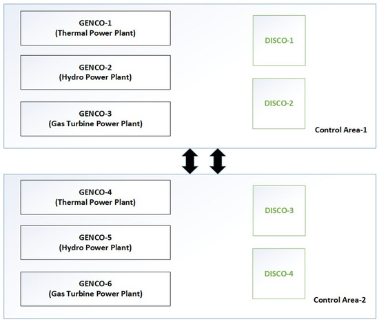
Figure 1. Pictorial representation of two-area deregulated power system.

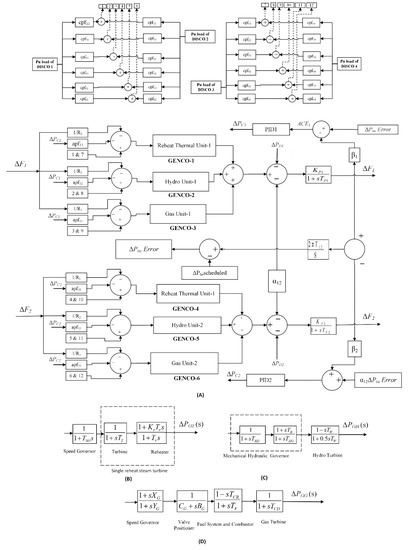
Figure 2. Restructured power system. TFM of (A) two-area multi-source restructured power system, (B) thermal system, (C) hydro system, (D) gas system.

Because each area has three GENCOs, the area control error (ACE) must be divided based on the AGC participation. Coefficients that distribute ACE to different GENCOs are termed as “ACE participation factors” (APF). We have considered APF as per the participation of respective GENCOs with the following participation factor values: apf11 = 0.6, apf12 = 0.3, apf13 = 0.1 for the first area, and apf21 = 0.6, apf22 = 0.3, apf23 = 0.1 for the second area.

In a deregulated environment, several DISCOs and GENCOs are interconnected, and each DISCO has a contract in its own area or another control area, and all these transactions have to be executed under the supervision of the ISO. The DISCO participation matrix (DPM) is a matrix that represents these various contracts. This DPM aids us in quickly identifying these contracts. As the name implies, DPM denotes DISCO’s participation in a contract with GENCO. As a result, the contract participation factor (CPF) for each ijth element of the matrix corresponds to the proportion of total load contracted by DISCO ‘$j$’ from GENCO ‘$i$’, and their total value is one, as given in Equation (1) The local demand is represented by diagonal elements in a DPM matrix, whereas the contribution from other regions is represented by off-diagonal elements. For example, CPF₁₂ means the demands of DISCO-2 from GENCO-1. The CPF can be written as follows:

$$\sum cp{f}_{ij}=1.0$$

(1)

The corresponding DPM related to three GENCOs along with two DISCOs in area-1 and three GENCOs along with two DISCOs in area-2 is shown in Equation (2):

$$DPM=\left[\begin{array}{c}cp{f}_{11} cp{f}_{12} cp{f}_{13} cp{f}_{14}\\ cp{f}_{21} cp{f}_{22} cp{f}_{23} cp{f}_{24}\\ cp{f}_{31} cp{f}_{32} cp{f}_{33} cp{f}_{34}\\ cp{f}_{41} cp{f}_{42} cp{f}_{43} cp{f}_{44}\\ cp{f}_{51} cp{f}_{52} cp{f}_{53} cp{f}_{54}\\ cp{f}_{61} cp{f}_{62} cp{f}_{63} cp{f}_{64}\end{array}\right]$$

(2)

If a DISCO’s load changes, it appears as a local load in the area to which it belongs, shown in Equation (3):

$$\mathsf{\Delta }{P}_{D1}=\mathsf{\Delta }{P}_{L1}+\mathsf{\Delta }{P}_{L2}, \mathsf{\Delta }{P}_{D2}=\mathsf{\Delta }{P}_{L3}+\mathsf{\Delta }{P}_{L4}$$

(3)

where $∆P_{D1}$ and $∆P_{D2}$ are the local loads of area-1 and area-2, respectively, and the values of $\mathsf{\Delta }{P}_{L1}, \mathsf{\Delta }{P}_{L2}, \mathsf{\Delta }{P}_{L3,} and \mathsf{\Delta }{P}_{L4}$ are the load values of DISCO-1, DISCO-2, DISCO-3, and DISCO-4, respectively.

The scheduled steady state tie-line power flow ($\mathsf{\Delta }{P}_{tie1-2,scheduled}$), $\mathsf{\Delta }{P}_{tie1-2,scheduled}$ = (Demand of DISCOs in area-2 from GENCOs in area-1) $-$ (Demand of DISCOs in area-1 from GENCOs in area-2), can be shown in Equation (4):

$$\mathsf{\Delta }{P}_{tie1-2,scheduled}={\displaystyle \sum }_{i=1}^3{\displaystyle \sum }_{j=3}^{4}cp{f}_{ij}\mathsf{\Delta }{P}_{Lj}-{\displaystyle \sum }_{i=4}^6{\displaystyle \sum }_{j=1}^{2}cp{f}_{ij}\mathsf{\Delta }{P}_{Lj}$$

(4)

The steady-state actual power ($\mathsf{\Delta }{P}_{tie1-2,actual}$) flowing through the tie line can be expressed as in Equation (5),

$$\mathsf{\Delta }{P}_{tie1-2,actual}=\frac{2\Pi T_{12}}{s}\left(\mathsf{\Delta }{F}_1-\mathsf{\Delta }{F}_2\right)$$

(5)

where $T_{12}$ is the tie-line synchronizing coefficient. The value of tie-line power error (ΔP_{tie1 − 2,} error) is shown in Equations (6) and (8):

$$\mathsf{\Delta }{P}_{tie1-2,error}=\mathsf{\Delta }{P}_{tie1-2,actual}-\mathsf{\Delta }{P}_{tie1-2,scheduled}$$

(6)

With the help of this tie-line power error we generate ACE signal, as shown in Equations (7) and (9):

$$e_1\left(t\right)=AC{E}_1={\beta }_1\mathsf{\Delta }{F}_1+\mathsf{\Delta }{P}_{tie1-2,error}, e_2\left(t\right)=AC{E}_2={\beta }_2\mathsf{\Delta }{F}_2+\mathsf{\Delta }{P}_{tie2-1,error}$$

(7)

$$\mathsf{\Delta }{P}_{tie2-1,error}={\alpha }_{12}\mathsf{\Delta }{P}_{tie1-2,error}$$

(8)

where${\alpha }_{12}=-\frac{p_{r1}}{p_{r2}}$, and $P_{r1}$ and $P_{r2}$ are the rated power of the respective areas.

Therefore,

$$AC{E}_2={\beta }_2\mathsf{\Delta }{F}_2+{\alpha }_{12}\mathsf{\Delta }{P}_{tie1-2,error}$$

(9)

where β₁ and β₂ represent the frequency biasing in area-1 and area-2, and ΔF₁ and ΔF₂ are the frequency deviations in area-1 and area-2, respectively. The TFM values and rated values of considered system are mentioned in Appendix A.

3. Proposed IGSA-BPSO Algorithm

The new improved gravitational search algorithm (IGSA) combines the features of a binary version of PSO with GSA. Hybrid intelligent optimization techniques include the specific quality of two well-known optimization techniques, such as GSA and binary version of PSO. Here, possible candidate solutions are termed as ‘objects’ and the position of each object is changed after each iteration depending on the properties of GSA and BPSO. GSA technique is inspired by gravitational law, and the performance of each candidate solution is based on the mass of each agent. Particle swarm optimization is used to update the particle’s position depending upon the particle’s velocity, and it is decided by the current particles best position and particles global best position.

The IGSA includes all the best properties of GSA and PSO for updating the values of each object after each iteration.

Let there be ‘N’ number of objects in ‘m’ dimensions, and the position of each object ‘$i$’ is denoted as Equation (10):

$$x_i=\left(x_i^1,.....x_i^d,......x_i^m\right)\mathrm{for}\mathrm{i}=1,2,\dots \mathrm{N}$$

(10)

Here, $x_i^d$ refers to the $i\mathrm{th}$ agent positioned in dth dimension. The updated position of the object is shown in Equation (11):

$$x_i{}^d\left(t+1\right)=x_i{}^d\left(t\right)+a_i^d\left(t\right)+v_i^d\left(t+1\right)+\alpha \epsilon$$

(11)

Here, $x_i{}^d\left(t\right)$ is the current position of object for iteration ‘$t$’ shown in Equation (11).

The second term of Equation (11) shows the change of the object’s position to the new value with the effect of gravitational law (GSA). Acceleration of the object can be calculated by Equation (12):

$$a_i^d\left(t\right)=\frac{F_i^d\left(t\right)}{M_{ii}\left(t\right)}$$

(12)

where $F_i^d$ is the force on a single object ‘$i$’, $a_i^d\left(t\right)$ is acceleration of the object ‘i’, and M_ii is the mass of the ith object; see Equation (13).

$$F_i^d\left(t\right)={\displaystyle \sum }_{j=1,j\ne i}^{N}ran{d}_j{F}_{ij}^d\left(t\right)$$

(13)

The force acting on mass $‘i’$ due to mass ‘j’, is given in Equation (14)

$$F_{ij}^d\left(t\right)=G\left(t\right)\frac{M_{pi}\left(t\right)\ast M_{aj}\left(t\right)}{R_{ij}\left(t\right)+\epsilon }\left(x_j^d\left(t\right)-x_i^d\left(t\right)\right)$$

(14)

Here, $M_{pi}$ is the passive gravitational mass related to the ith agent, $M_{aj}$ is the active gravitational mass of the jth agent (14), $\epsilon$ is a small constant, $G\left(t\right)$ is the gravitational constant, and $R_{ij}$ is the Euclidian distance between agent $i$ and agent $j$, as given in Equation (15):

$$G\left(t\right)=G\left(G_0,t\right), R_{ij}\left(t\right)=|\left|X_i\left(t\right),X_j\left(t\right)\right|{|}_2$$

(15)

Masses of each agent are updated by Equation (16):

$$m_i\left(t\right)=\frac{fi{t}_i\left(t\right)-worst\left(t\right)}{best\left(t\right)-worst\left(t\right)};M_i\left(t\right)=\frac{m_i\left(t\right)}{{{\displaystyle \sum }}_{j=1}^N{m}_j\left(t\right)}$$

(16)

The third term of Equation (11) shows the velocity of each object updated based on PSO optimization techniques, where:

$$v_{id}{}^{t+1}=v_{id}{}^t+r1c1\left(pbes{t}^t-x_{id}{}^t\right)+r2c2\left(gbes{t}^t-x_{id}{}^t\right)$$

(17)

The variable S is the sigmoid function, as shown in Equation (18):

$$S\left(v_{id}{}^t\right)=\frac{1}{1+exp(-v_{id}{}^t)}$$

(18)

$$x_{id}^t=\left\{\begin{array}{c}1, \mathrm{if}\mathrm{rand}<\mathrm{S}\left(v_{id}{}^t\right)\\ 0,\mathrm{otherwise}\end{array}\right.$$

(19)

The variable $pbest$ is personal best of agent $i$, $gbest$ is global best, $r1$ and $r2$ are random numbers in [0, 1], $c1$ and $c2$ are acceleration coefficients, $x_{id}$ is position of the ith agent in dimension $d$, and $v_{id}{}^t$ is the velocity of the ith agent in dimension $d$ for iteration $t$, shown in Equation (19). The final term depicts the random movement of object to explore the new possible solutions.

4. Proposed Control Approach Methodology

A brief description related to the objective function, PID controller, and implementation of the proposed technique are presented in this section.

4.1. PID Controller

The most popular type of feedback controller in the industrial sector is PID controllers. There are so many benefits related to PID control, such as it has wide range of applications, is reliable, easy to understand, and easy to tune, but it has some limitations, such as process dynamics and time delay. PID is a single input and single output system. The PID controller’s output can be written as shown in Equation (20):

$$u\left(t\right)=K_{pr}e\left(t\right)+K_i\int e\left(t\right)dt+K_d\frac{de\left(t\right)}{dt}$$

(20)

where$K_i$, and $K_d$ are the proportional, integral, and derivative components belonging to the PID controller.

4.2. Objective Function

An IGSA-BPSO tuned PID controller is used for the performance analysis of the considered model. For an objective function, ITAE is taken into consideration, as shown in Equation (21).

$$J=ITAE={{\displaystyle \int }}_0^{t_{sim}}(\left|∆F_1\right|+\left|∆F_2\right|+\left|∆P_{tie}\right|)tdt$$

(21)

where ‘$t_{sim}$’ is the simulation time in (21) and has been set to 60 s. As shown in Equation (21), the tuning parameters of PID controllers are determined by minimizing the objective function.

4.3. Implementation of Proposed Concept

The proposed research work on an LFC for two-area multiple sources is presented in Figure 3. The detailed modeling is given in Section 2. In this paper, a robust PID controller is designed using a hybrid improved IGSA-BPSO algorithm proposed for optimally designing the suggested controller. In the optimization process, ITAE has been implemented as an objective function for improving optimal parameter selection of the proposed controller.

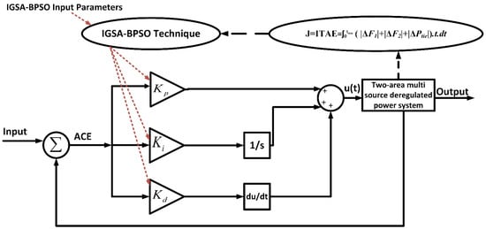
Figure 3. Schematic of proposed control scheme for the whole combined structure.

Several optimization techniques are used to determine the parameters for a PID controller. Each of these values $(K_p ,K_i$, and $K_d)$ is generated within the allowed range, as in Equation (22).

$$K_p^{min}\le K_p\le K_p^{max}, K_i^{min}\le K_i\le K_i^{max}, K_d^{min}\le K_d\le K_d^{max}$$

(22)

The PID controller’s value is kept within the range from 0.01 to 10. The parameters of different optimization techniques are kept as follows: the number of particles is 25 and the maximum iteration is 30. The flowchart of the detailed procedure is given in Figure 4.

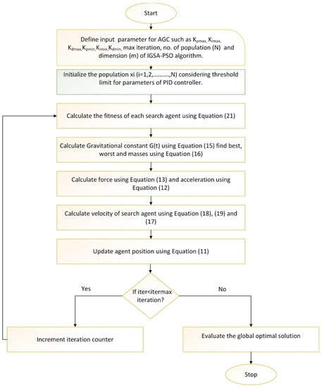
Figure 4. IGSA-BPSO flowchart of the detailed procedure.

5. Results and Discussion

In this section, simulation results are investigated for the aforementioned system. The deregulated system is studied for different possible contract agreements. For the performance analysis, simulations are performed in the MATLAB/Simulink environment.

To simulate all three cases of PBT, BBT, and CVT in a deregulated environment, the optimal regulators are designed in the present work are shown below:

5.1. Poolco Based Transaction (PBT)

For the PBT part of the deregulated power system, we assume that load changes only in area-1. Consequently, only the DISCO of area-1 demands the load. Therefore, CPFs in the DPM matrix for DISCO-3 and DISCO-4 are zero, because these DISCOs do not demand any load from GENCOs. For this case, we assume that DISCO-1 and DISCO-2 demand a load of 0.005 p.u. MW. The DPM can be summarized as follows:

$$\mathrm{DPM}=\left[\begin{array}{c}0.3333 0.3333 0 0\hfill \\ 0.3333 0.3333 0 0\hfill \\ 0.3333 0.3333 0 0\hfill \\ 0 0 0 0\\ 0 0 0 0\\ 0 0 0 0\end{array}\right]$$

(23)

In general cases, the desired power generated by each GENCOs in p.u. MW is explained as

$$∆P_{GENCO-i}=cp{f}_{i1}∆P_{L1}+cp{f}_{i2}∆P_{L12}+cp{f}_{i3}∆P_{L3}+cp{f}_{i4}∆P_{L4}$$

(24)

With the help of the aforementioned equation, we get the mathematical values of power generated by each GENCO under the steady state condition for the PBT case:

$$∆P_{GENCO-1}=0.3333\times 0.005+0.3333\times 0.005+0\times 0+0\times 0=0.003333 p.u.MW$$

(25)

Similarly,

ΔP_GENCO-2 = ΔP_GENCO-3 = 0.003333 p.u.MW & ΔP_GENCO-4 = ΔP_GENCO-5 = ΔP_GENCO-6 = 0 p.u. MW

When simulations are carried out, PID controller gains are optimized using GSA, PSO, and the suggested IGSA-BPSO algorithms, as illustrated in Table 1. Settling time and overshoot values of ΔF₁, ΔF₂, and ΔP_tie for GSA tuned PID, PSO tuned PID, and IGSA-BPSO tuned PID controllers are given in Table 2 and Table 3, respectively. Settling time value is showing better results as compare to the other two techniques. ITAE value of GSA tuned PID, PSO tuned PID, and IGSA-BPSO tuned PID are 0.0625, 0.0634, and 0.0445, respectively. The best ITAE value is with the recommended hybrid IGSA-BPSO tuned PID controllers, as shown in Table 1. The responses in Figure 5a–f established that the proposed controller performs better than GSA-PID and PSO-PID in terms of settling time.

Table 1. PID Parameters tuning for hybrid test system and ITAE values: PBT.

S.no	Gain	GSA_PID	PSO_PID	IGSA-BPSO_PID
1	Kp1	1.6945	2.5173	3.8121
2	Ki1	6.5164	4.0844	10.0000
3	Kd1	1.8420	3.7709	3.0016
4	Kp2	0.0100	0.3234	0.1000
5	Ki2	5.2595	0.1000	7.9759
6	Kd2	5.1371	1.2636	5.5663
ITAE		0.0625	0.0634	0.0445

Table 2. Settling time values(s) for different optimization techniques (O.T.)–PBT.

S.no	State Variables	GSA_PID	PSO_PID	IGSA-BPSO_PID
1	ΔF1	3.9716	5.8498	3.8680
2	ΔF2	9.0694	9.5832	7.8890
3	ΔPtie	7.4691	14.2268	6.6363
4	ΔPg1	40.6566	37.2204	36.9693
5	ΔPg2	39.4633	37.3227	36.7012
6	ΔPg3	19.5268	21.7294	17.9643

Table 3. Overshoot values(s) for different optimization techniques (O.T.)–PBT.

S.no	State Variables	GSA_PID (p.u.)	PSO_PID (p.u.)	IGSA-BPSO_PID (p.u.)
1	ΔF1	−0.015622	−0.014892	−0.015120
2	ΔF2	−0.006726	−0.004628	−0.005288
3	ΔPtie	−0.019728	−0.014282	−0.014126
4	ΔPg1	0.009276	0.012000	0.012000
5	ΔPg2	0.004277	0.006228	0.006240
6	ΔPg3	0.007624	0.007224	0.007120

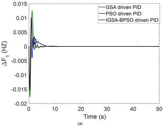
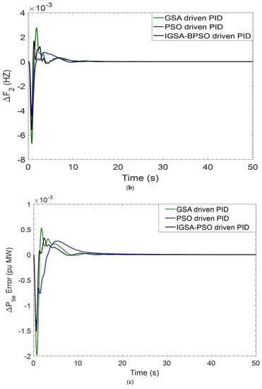
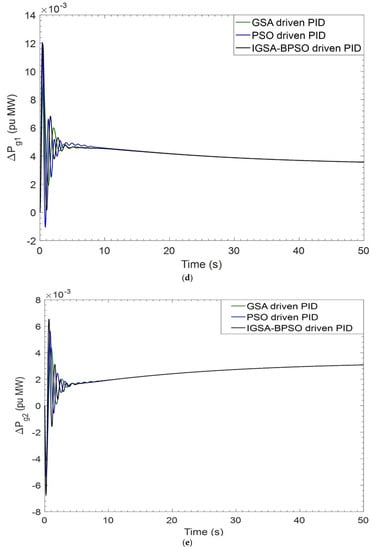
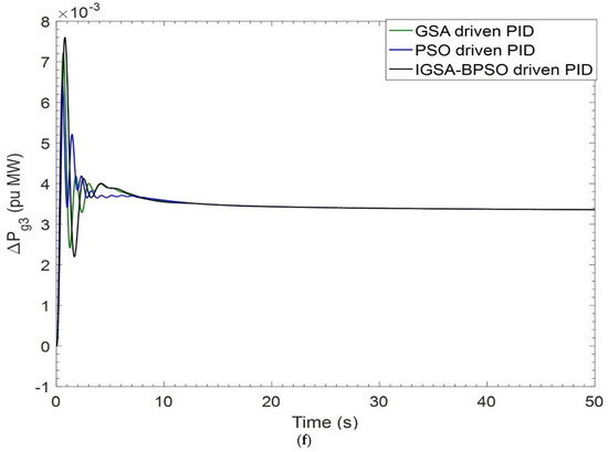
Figure 5. (a) Deviation in frequency ΔF₁ for PBT case; (b) deviation in frequency ΔF₂ for PBT case; (c) deviation in tie-line power ΔP_tie for PBT case; (d) deviation in power related to GENCO—1 for PBT case; (e) deviation in power related to GENCO—2 for PBT case; (f) deviation in power related to GENCO—3 for PBT case.

5.2. Bilateral Based Transaction (BBT)

This contract allows a DISCO to buy power for GENCOs in their own area and purchase power from GENCOs in other areas. In this case, we assume that a load deviation of 0.01 p.u. MW occurred in both areas. Therefore, each DISCO demanded 0.005 p.u. MW. The CPFs related to the BBT case are shown in the following DPM matrix.

$$\mathrm{DPM}=\left[\begin{array}{c}0.2 0.1 0.3 0.0000\\ 0.2 0.2 0.1 0.1666\\ 0.1 0.3 0.1 0.1666\\ 0.2 0.1 0.1 0.3336\\ 0.2 0.2 0.2 0.1666\\ 0.1 0.1 0.2 0.1666\end{array}\right]$$

(26)

The power outputs related to every GENCO may be written as follows:

$$∆P_{GENCO-i}=cp{f}_{i1}\mathsf{\Delta }{P}_{L1}+cp{f}_{i2}\mathsf{\Delta }{P}_{L12}+cp{f}_{i3}\mathsf{\Delta }{P}_{L3}+cp{f}_{i4}\mathsf{\Delta }{P}_{L4}$$

(27)

where

$$\begin{array}{c}∆P_{GENCO-1}=0.2\times 0.005+0.1\times 0.005+0.3\times 0.005+0\times 0.005=0.0033p.u.MW\\ ∆P_{GENCO-2}=0.2\times 0.005+0.2\times 0.005+0.1\times 0.005+0.1666\times 0.005=0.00333p.u.MW\\ ∆P_{GENCO-3}=0.1\times 0.005+0.3\times 0.005+0.1\times 0.005+0.1666\times 0.005=0.00333p.u.MW\\ ∆P_{GENCO-4}=0.2\times 0.005+0.1\times 0.005+0.1\times 0.005+0.3336\times 0.005=0.003668p.u.MW\\ ∆P_{GENCO-5}=0.2\times 0.005+0.2\times 0.005+0.2\times 0.005+0.1666\times 0.005=0.003833p.u.MW\\ ∆P_{GENCO-6}=0.1\times 0.005+0.1\times 0.005+0.2\times 0.005+0.1666\times 0.005=0.00283p.u.MW\end{array}$$

When simulations are carried out, PID controller gains are optimized using GSA, PSO, and the suggested IGSA-BPSO algorithms, as illustrated in Table 4. Settling time and overshoot values of ΔF₁, ΔF₂, and ΔP_tie for GSA tuned PID, PSO tuned PID, and IGSA-BPSO tuned PID controllers are given in Table 5 and Table 6, respectively. The settling time is showing better results as compared to the other two techniques. ITAE values of GSA tuned PID, PSO tuned PID, and IGSA-BPSO tuned PID are 0.1491, 0.0789, and 0.0626, respectively. The ITAE has the lowest value with the recommended hybrid IGSA-BPSO tuned PID controllers, as shown in Table 4. The dynamic responses obtained in Figure 6a–i show that the proposed controller outperforms GSA_PID and PSO_PID in settling time.

Table 4. PID parameters tuning for hybrid test system and ITAE values: BBT.

S.no	Gain	GSA_PID	PSO_PID	IGSA-BPSO_PID
1	Kp1	1.2849	3.8659	4.4134
2	Ki1	5.6178	9.9224	10.0000
3	Kd1	2.5133	2.7400	3.7194
4	Kp2	0.0100	2.9729	4.5451
5	Ki2	4.0319	8.5635	9.9999
6	Kd2	4.4431	4.4094	3.6438
ITAE		0.1491	0.0789	0.0626

Table 5. Settling time values (s) for different optimization techniques (O.T.)—BBT.

S.no	State Variables	GSA_PID	PSO_PID	IGSA-BPSO_PID
1	ΔF1	8.1157	4.8904	3.0674
2	ΔF2	5.7913	4.5854	3.5205
3	ΔPtie	16.2146	7.3113	5.4959
4	ΔPg1	40.5425	37.6034	36.3051
5	ΔPg2	39.1134	38.0370	36.7099
6	ΔPg3	19.4106	17.3827	15.2442
7	ΔPg4	39.8280	38.2706	38.1125
8	ΔPg5	37.6308	37.6084	37.0393
9	ΔPg6	21.2714	23.3137	21.2218

Table 6. Overshoot values (s) for different optimization techniques (O.T.)–BBT.

S.no	State Variables	GSA_PID	PSO_PID	IGSA-BPSO_PID
1	ΔF1	−0.019233	−0.015560	−0.149832
2	ΔF2	−0.009236	0.008232	−0.015200
3	ΔPtie	−0.014821	−0.014221	−0.015122
4	ΔPg1	0.009000	0.011623	0.012242
5	ΔPg2	−0.004822	0.006000	−0.006322
6	ΔPg3	0.007412	0.007822	0.007010
7	ΔPg4	0.011227	0.013271	0.012748
8	ΔPg5	−0.006621	−0.007242	−0.006427
9	ΔPg6	0.006421	0.006124	0.006824

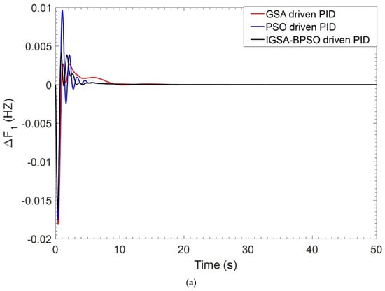
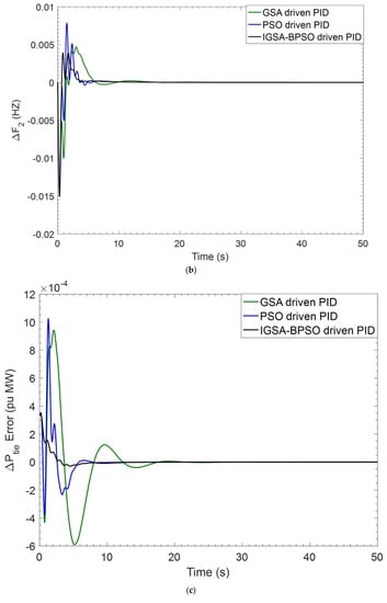
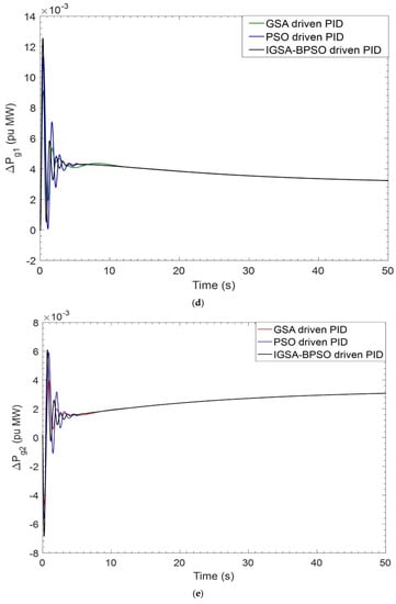
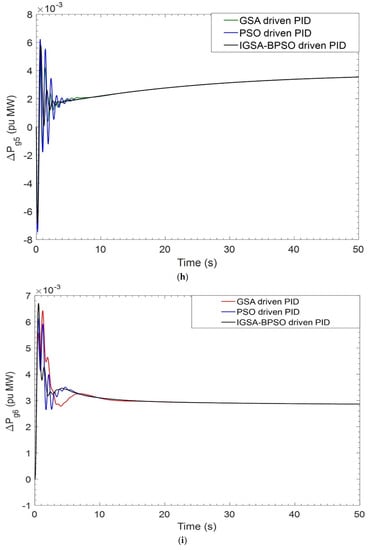
Figure 6. (a) Dynamic response of ΔF₁ for BBT case; (b) dynamic response of ΔF₂ for BBT case; (c) dynamic response of ΔP_tie for BBT case; (d) perturbation response of GENCO–1 for BBT case; (e) perturbation response of GENCO-2 for BBT case; (f) perturbation response of GENCO-3 for BBT case; (g) perturbation response of GENCO-4 for BBT case; (h) perturbation response of GENCO-5 for BBT case; (i) perturbation response of GENCO-6 for BBT case.

5.3. Contract Violation Based Transaction (CVBT)

DISCOs sometimes demand more excess power than the contract agreement specifies. The excess power should not be shown as contracted demands but should be replicated as local load of that area and supplied by GENCOs of the same area. For this special case of deregulation contracts violation, we consider DISCO-1 demand 0.003 p.u. extra un-contracted power demand. As there are load changes only in area one, the corresponding GENCOs change and there are no GENCOs corresponding to area two, as no load changes in area two. Values of respective APFs in area-1 decides involvement of un-contracted load amongst GENCOs in that area.

Therefore, the local load of area-1 = (Contracted load of DISCO-1 $+$ Contracted load of DISCO-2 $+$ uncontracted_load) = (0.005$+$0.005$+$0.003) = 0.013 p.u. M.W.

The total load in area-2 = (Contracted load of DISCO-3 $+$ Contracted load of DISCO-4 $+$ uncontracted_load) = (0.005 + 0.005 + 0) = 0.01 p.u.M.W.

$$\begin{array}{c}∆P_{GENCO-i}=\left(cp{f}_{i1}∆P_{L1}+cp{f}_{i2}∆P_{L12}+cp{f}_{i3}∆P_{L3}+cp{f}_{i4}∆P_{L4}\right)+\left(ap{f}_{respective}\times uncontracte{d}_{demand}\right)\\ ∆P_{GENCO-1}=\left(0.2\times 0.005+0.1\times 0.005+0.3\times 0.005+0\times 0.005\right)+\left(0.6\times 0.003\right)=0.0048p.u.MW\\ ∆P_{GENCO-2}=\left(0.2\times 0.005+0.2\times 0.005+0.1\times 0.005+0.1666\times 0.005\right)+\left(0.3\times 0.003\right)=0.00423p.u.MW\\ ∆P_{GENCO-3}=\left(0.1\times 0.005+0.3\times 0.005+0.1\times 0.005+0.1666\times 0.005\right)+\left(0.1\times 0.003\right)=0.00363p.u.MW\end{array}$$

(28)

The un-contracted load demanded by DISCO-1 and DISCO-2 does not affect the GENCOs of area two. The dynamic responses in Figure 7a–f indicate better performance of the proposed controller as compared with GSA: PID and PSO: PID in settling time. ITAE values of GSA tuned PID, PSO tuned PID, and IGSA-BPSO tuned PID are 0.0792, 0.2749, and 0.0750, respectively. When simulation is carried out, PID controller gains are optimized using GSA, PSO, and the suggested IGSA-BPSO algorithms, as illustrated in Table 7. The settling time and overshoot values of ΔF₁, ΔF₂, and ΔP_tie for GSA tuned PID, PSO tuned PID, and IGSA-BPSO tuned PID controllers are given in Table 8 and Table 9, respectively.

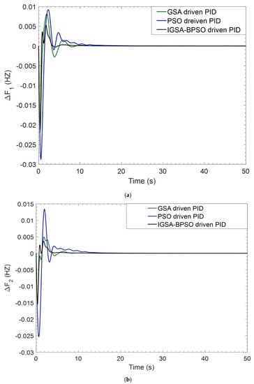
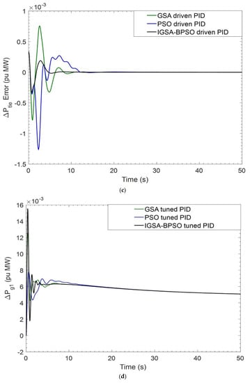
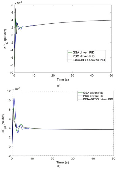
Figure 7. (a) Dynamic response of ΔF₁ for CVT case; (b) dynamic response of ΔF₂ for CVT case; (c) dynamic response of ΔP_tie for BBT case; (d) perturbation response of GENCO-1 for CVT case; (e) perturbation response of GENCO-2 for CVT case; (f) perturbation response of GENCO-3 for CVT case.

Table 7. PID parameters tuning for hybrid test system and ITAE values: CVT.

S.no	Gain	GSA_PID	PSO_PID	IGSA-BPSO_PID
1	Kp1	4.5030	0.0100	3.1433
2	Ki1	8.9505	2.2039	9.7678
3	Kd1	3.1348	1.2636	3.6908
4	Kp2	3.5816	0.0100	4.7799
5	Ki2	7.5926	2.5565	10.0000
6	Kd2	3.3556	0.8327	3.5958
ITAE		0.0792	0.2749	0.0750

Table 8. Settling time values (s) for different optimization techniques (O.T.)–CVT.

S.no	State Variables	GSA_PID	PSO_PID	IGSA-BPSO_PID
1	ΔF1	5.3970	9.1038	3.0820
2	ΔF2	5.9101	10.5107	3.7475
3	ΔPtie	8.4441	11.6452	6.6799
4	ΔPg1	37.2376	43.0116	37.2357
5	ΔPg2	37.0082	40.9731	36.5868
6	ΔPg3	17.6353	19.0666	10.4262

Table 9. Overshoot values (s) for different optimization techniques (O.T.) on system state variables–CVT.

S.no	State Variables	GSA_PID	PSO_PID	IGSA-BPSO_PID
1	ΔF1	−0.023172	−0.021271	−0.028718
2	ΔF2	−0.015252	−0.025000	−0.014176
3	ΔPtie	0.003812	−0.001278	−0.000321
4	ΔPg1	0.015827	0.007827	0.015728
5	ΔPg2	0.007892	−0.003426	−0.008178
6	ΔPg3	0.009237	0.010268	0.008523

All three techniques are also compared based on their convergence characteristics. The convergence characteristics of all three techniques are shown in Figure 8.

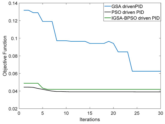
Figure 8. Convergence characteristics for different techniques.

6. Different Cases Related to Uncertainties and Dynamic Changes

6.1. Sensitivity Analysis

In this paper, sensitivity analysis is performed to test the proposed system’s robustness against small changes in system parameters. As the parameter changes over time as a result of system wear and tear, and also due to inaccurate system modelling, the designed controller must be robust to sustain the variation in parameters such as (T_SG) thermal speed governor time constant, (T_RH) hydro turbine speed governor time constant, and (X_G) lead time constant of gas turbine speed governor, which are deviated ±25% from nominal values. The results indicate that the values of settling time and overshoot change with the change of parameters, but still they remain within the noted limits, as shown in Figure 9a–c.

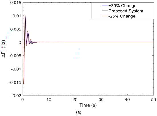
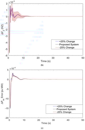
Figure 9. (a) Perturbation response of frequency (ΔF₁) with ±25 change in T_SG parameter; (b) perturbation response of frequency (ΔF₂) with ±25 change in T_RH parameter; (c) perturbation response of tie-line power (ΔP_tie) with ±25 change in X_G parameter.

6.2. Nonlinearities

In the second case, we have incorporated nonlinearities such as GRC and TD in the proposed system, and the simulation results are compared to the system having no nonlinearities. In the non-appearance of GRC, generators are expected to follow large momentary disturbances. Consequently, GRC should be considered in any realistic AGC study. For the thermal system, we have taken a GRC of 10% per minute (0.0017 p.u. MW/s) for falling and rising in this unit. For the hydro unit, we have assumed a GRC of 270% per minute (0.045 p.u. MW/s) for falling and 360% per minute (0.06 p.u. MW/s) for rising in this unit [49].

As in the restructured scenario of an interconnected power system, AGC performance analysis becomes challenging due to delays in communication channels, as it causes system instability. Based on the above, a time delay of 0.03 s is taken into account for the system to evaluate the sensitivity of nonlinearities [50].

The system dynamics results related to nonlinearities added to the system are shown in Figure 10a–f. The investigation of simulation results after the addition of nonlinearities witnessed no sign of instability.

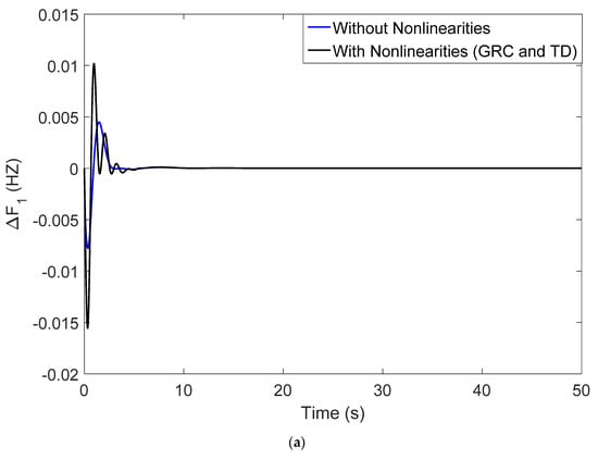
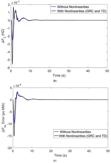
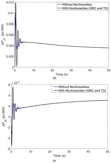
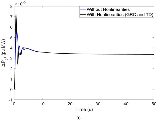
Figure 10. (a) Perturbation response (ΔF₁) with and without (GRC and TD); (b) perturbation response (ΔF₂) with and without (GRC and TD); (c) perturbation response (ΔP_tie) with and without (GRC and TD); (d) perturbation response (ΔP_g1) with and without (GRC and TD); (e) perturbation response (ΔP_g2) with and without (GRC and TD); (f) perturbation response (ΔP_g3) with and without (GRC and TD).

6.3. Dynamic Load Changes

In the third case, we added the variable load changes condition. For this part, at the initial time, DISCO-1 of area one demands 0.005 p.u. MW; at the 20th second, it demands 0.004 p.u. MW; and at the 40th second, it demands 0.006 p.u. MW. For the overall DISCOs of area-1, at initial time, they demand 0.01 p.u. MW; at the 20th second, they demand 0.009 p.u. MW; and at the 40th second, they demand 0.011 p.u. MW. These results can be seen in Figure 11a,b. All three optimization techniques compare for the PBT case, and the system shows stable conditions even after the changes of load at the different time schedules.

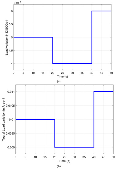
Figure 11. (a) Dynamic load changes for DISCO-1; (b) dynamic load changes for area-1.

The proposed system’s adaptability has been addressed by altering the load in DISCO-1 and area-1 after a 20 s interval. Whenever we change load in DISCO-1, it directly effects area-1. In this part of the dynamic load variation, our consideration is related to area-1. The proposed concept for handling the LFC problem improves the system dynamics, reliability, and flexibility of the power system to accommodate dynamical changes in the load at regular intervals, as shown in Figure 12a–f.

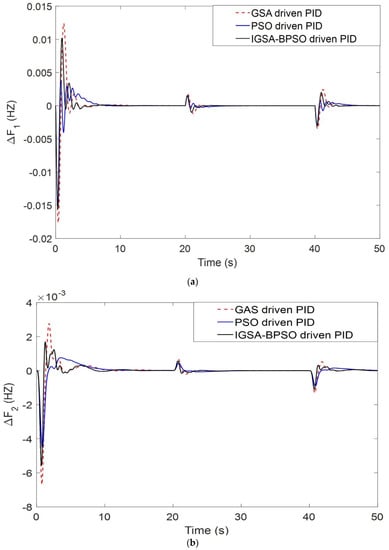
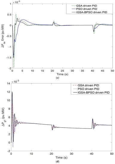
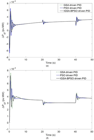
Figure 12. (a) Dynamic load changes variation for ΔF₁ related to PBT case; (b) dynamic load changes variation for ΔF₂ related to PBT case; (c) dynamic load changes variation for ΔP_tie related to PBT case; (d) dynamic response ΔP_g1 for PBT case; (e) dynamic response ΔP_g2 for PBT case; (f) dynamic response ΔP_g3 for PBT case.

Even after the changing of load demand of any of the DISCOs at any time, the proposed system showed a stability condition. Responses are shown in Figure 12a–f. In this part, we change the dynamic load condition for DISCO–1 of area one for the poolco based transaction, and the results are compared for all three techniques. The proposed technique shows lower settling time compared to the other two techniques [51].

6.4. AC-DC Tie-Line Analysis

The AC transmission lines are used for transferring electrical power from one power station to different load centers, but at high voltage level, they experienced many problems. Figure 13 depicts the modelling of the AC-DC tie line for a two-area power system. The firing angles of the rectifier and inverter must be equal for transfer of equal power from both sides of the DC tie line [52,53]. An AC-DC parallel link helped the tie-line power exchange, and it also helped in controlling the power transfer. Responses of AC-DC tie-line impact are shown in Figure 14a–f. All cases are considered for PBT.

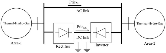
Figure 13. AC-DC parallel links for the considered system.

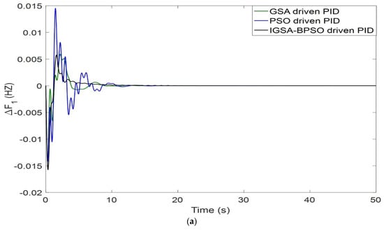
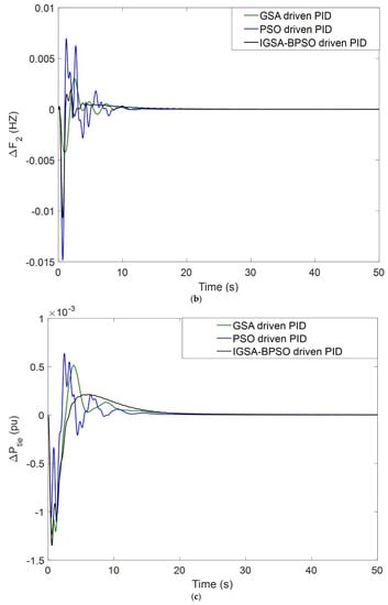
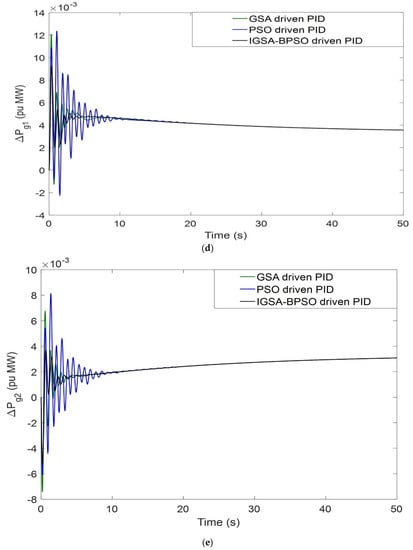
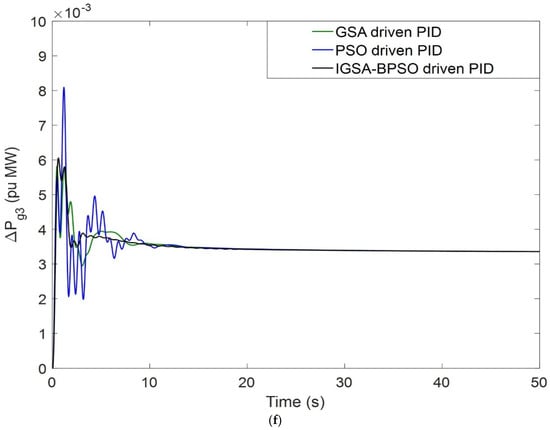
Figure 14. (a) Dynamic responses of ΔF₁ under addition of AC-DC tie line; (b) dynamic responses of ΔF₂ under addition of AC-DC tie line; (c) dynamic responses of ΔP_tie under addition of AC-DC tie line; (d) dynamic responses of ΔP_g1 under addition of AC-DC tie line; (e) dynamic responses of ΔP_g2 under addition of AC-DC tie line; (f) dynamic responses of ΔP_g3 under addition of AC-DC tie line.

The above mentioned four different cases are mentioned in Table 10. The variation in different parameters corresponding changes of all the parameters are summarized and their results are also discussed in Table 10.

Table 10. Summary results for different cases related to uncertainties and dynamic changes.

No.	Different Cases	Variation in Different Parameters	Results
1	Sensitivity analysis	(TSG), (TRH) and (XG) parameters of gas unit-1 and gas unit-2, which deviate ±25% from nominal values.	Value of settling time and overshoot changes with the change of the parameters; however, it remains within limits.
2	Nonlinearities	(i) GRC of ±10% per minute for the thermal unit. The hydro unit GRC of 270% per minute (0.045 p.u. MW/s) for falling and 360% per minute (0.06 p.u. MW/s) for rising in this unit. (ii) TD of 0.03 s.	A realistic view of the power system is shown by considering different nonlinearities such as GRC and TD.
3	Dynamic load changes	DISCOs of area-1 at initial time demanding 0.01 p.u. MW, at 20th second demanding 0.009 p.u. MW, and at 40th second demanding 0.011 p.u. MW.	The system shows stable condition even after changing the load at different scheduled times.
4	AC-DC tie-line analysis	Parallel AC-DC tie link in place of AC tie line.	AC-DC parallel link help in tie-line power exchange, and it also helps in controlling the power transfer.

7. Conclusions

This article proposes a novel IGSA-BPSO-driven PID controller concept for LFC of multi-area multi-sources test under the deregulated regime. A hybrid two-area system includes thermal, hydro, and gas turbine power plants. The proposed IGSA-BPSO technique is used to optimize the PID controller parameters by minimizing ITAE as the objective function. Different system nonlinearities such as GRC and TD are considered to have a realistic approach. A modified test system with a parallel AC-DC tie line to increase the power transfer capability and quick power modulation are considered and analyzed with the proposed concept. To analyze the robustness of the concept, dynamic load change with respect to time is considered for different deregulated power transactions, such as PBT, BBT, and CVT. The results have been studied and analyzed compared to PSO and GSA-driven PID controllers. The proposed IGSA-BPSO-driven PID controller shows the superiority to the other two techniques in settling time, overshoot, and convergence time. In the case of adding nonlinearities (GRC-TD), the simulation results showed no sign of instability, making the overall controller more economical compared to the other controllers. In the case of dynamic load changes, the proposed controller shows a stable system. This proposed algorithm mainly applies to the small perturbation in the load demand resulting in frequency and tie-line power deviations. If there are significant changes in load or a large disturbance, as in the case of fault, the proposed technique is not applicable because of the linear modeling of the system. The linear structure of classical PID controllers makes them ineffective for higher-order time delay systems. This can be eliminated by using advanced controllers tuned with intelligent meta-heuristic optimization techniques.

References

- Kundur, P. Power System Stability and Control; Balu, N.J., Lauby, M.G., Eds.; McGraw-Hill Education: New York, NY, USA, 1994; Chapter 4.2. [Google Scholar]
- Ibraheem; Kumar, P.; Kothari, D.P. Recent philosophies of automatic generation control strategies in power systems. IEEE Trans. Power Syst. 2005, 20, 346–357. [Google Scholar] [CrossRef]
- Shah, R.; Sanchez, J.C.; Preece, R.; Barnes, M. Stability and control of mixed AC–DC systems with VSC-HVDC: A review. IET Gener. Transm. Distrib. 2018, 12, 2207–2219. [Google Scholar] [CrossRef]
- Gupta, D.K.; Jha, A.; Appasani, B.; Srinivasulu, A.; Bizon, N.; Thounthong, P. Load Frequency Control Using Hybrid Intelligent Optimization Technique for Multi-Source Power Systems. Energies 2021, 14, 1581. [Google Scholar] [CrossRef]
- Kumari, S.; Shankar, G. Novel application of integral-tilt-derivative controller for performance evaluation of load frequency control of interconnected power system. IET Gener. Transm. Distrib. 2018, 12, 3550–3560. [Google Scholar] [CrossRef]
- Ma, M.; Liu, X.; Zhang, C. LFC for multi-area interconnected power system concerning wind turbines based on DMPC. IET Gener. Transm. Distrib. 2017, 11, 2689–2696. [Google Scholar] [CrossRef]
- Shankar, R.; Pradhan, S.; Chatterjee, K.; Mandal, R. A comprehensive state of the art literature survey on LFC mechanism for power system. Renew. Sustain. Energy Rev. 2017, 76, 1185–1207. [Google Scholar] [CrossRef]
- Das, A.; Dawn, S.; Gope, S.; Ustun, T.S. A Strategy for System Risk Mitigation Using FACTS Devices in a Wind Incorporated Competitive Power System. Sustainability 2022, 14, 8069. [Google Scholar] [CrossRef]
- Chinmoy, L.; Iniyan, S.; Goic, R. Modeling wind power investments, policies and social benefits for deregulated electricity market—A review. Appl. Energy 2019, 242, 364–377. [Google Scholar] [CrossRef]
- Mishra, R.N.; Chaturvedi, D.K.; Kumar, P. Recent philosophies of AGC techniques in deregulated power environment. J. Inst. Eng. Ser. B 2020, 101, 417–433. [Google Scholar] [CrossRef]
- Teresa, D.; Krishnarayalu, M.S. On deregulated power system AGC with solar power. Int. J. Comput. Appl. 2019, 45, 0975–8887. [Google Scholar] [CrossRef]
- Sannigrahi, S.; Ghatak, S.R.; Basu, D.; Acharjee, P. Optimal placement of DSTATCOM, DG and their performance analysis in deregulated power system. Int. J. Power Energy Convers. 2019, 10, 105–128. [Google Scholar] [CrossRef]
- Donde, V.; Pai, M.A.; Hiskens, I.A. Simulation and optimization in an AGC system after deregulation. IEEE Trans. Power Syst. 2001, 16, 481–489. [Google Scholar] [CrossRef]
- Parmar, K.P.; Singh, S.M.; Kothari, D.P. LFC of an interconnected power system with multi-source power generation in deregulated power environment. Int. J. Electr. Power Energy Syst. 2014, 57, 277–286. [Google Scholar] [CrossRef]
- Hota, P.K.; Mohanty, B. Automatic generation control of multi source power generation under deregulated environment. Int. J. Electr. Power Energy Syst. 2016, 75, 205–214. [Google Scholar] [CrossRef]
- Sekhar, G.T.C.; Sahu, R.K.; Baliarsingh, A.; Panda, S. Load frequency control of power system under deregulated environment using optimal firefly algorithm. Int. J. Electr. Power Energy Syst. 2016, 74, 195–211. [Google Scholar] [CrossRef]
- Kumar, R.; Sharma, V.K. Whale optimization controller for load frequency control of a two-area multi-source deregulated power system. Int. J. Fuzzy Syst. 2020, 22, 122–137. [Google Scholar] [CrossRef]
- Das, M.K.; Bera, P.; Sarkar, P.P. PID-RLNN controllers for discrete mode LFC of a three-area hydrothermal hybrid distributed generation deregulated power system. Int. Trans. Electr. Energy Syst. 2021, 31, e12837. [Google Scholar] [CrossRef]
- Selvaraju, R.K.; Somaskandan, G. Impact of energy storage units on load frequency control of deregulated power systems. Energy 2016, 97, 214–228. [Google Scholar] [CrossRef]
- Konar, G.; Mandal, K.K.; Chakraborty, N. Two area load frequency control using GA tuned PID controller in deregulated environment. In Proceedings of the International MultiConference of Engineers and Computer Scientists, Hong Kong, China, 12–14 March 2014; IAENG: Hong Kong, China, 2014; Volume 2. [Google Scholar]
- Arya, Y.; Kumar, N. AGC of a multi-area multi-source hydrothermal power system interconnected via AC/DC parallel links under deregulated environment. Int. J. Electr. Power Energy Syst. 2016, 75, 127–138. [Google Scholar] [CrossRef]
- Ma, M.; Zhang, C.; Liu, X.; Chen, H. Distributed model predictive load frequency control of the multi-area power system after deregulation. IEEE Trans. Ind. Electron. 2017, 64, 5129–5139. [Google Scholar] [CrossRef]
- Nayak, N.; Mishra, S.; Sharma, D.; Sahu, B.K. Application of modified sine cosine algorithm to optimally design PID/fuzzy-PID controllers to deal with AGC issues in deregulated power system. IET Gener. Trans. Distrib. 2019, 13, 2474–2487. [Google Scholar] [CrossRef]
- Kouba, N.E.Y.; Menaa, M.; Hasni, M.; Boussahoua, B.; Boudour, M. Optimal Load Frequency Control in Interconnected Power System Using PID Controller Based on Particle Swarm Optimization. In Proceedings of the 2014 International Conference on Electrical Sciences and Technologies in Maghreb (CISTEM), Tunis, Tunisia, 3–6 November 2014; IEEE: Piscataway, NJ, USA, 2014. [Google Scholar]
- Jha, A.V.; Gupta, D.K.; Appasani, B. The PI Controllers and Its Optimal Tuning for Load Frequency Control (LFC) of Hybrid Hydro-Thermal Power Systems. In Proceedings of the 2019 International Conference on Communication and Electronics Systems (ICCES), Coimbatore, India, 17–19 July 2019; IEEE: Piscataway, NJ, USA, 2019. [Google Scholar]
- Kumar, A.; Gupta, D.K.; Ghatak, S.R. GSA Based PID Controller for Load Frequency Control of Multi-Area Hybrid Power System. In Proceedings of the 2021 International Conference on Emerging Techniques in Computational Intelligence (ICETCI), Hyderabad, India, 25–27 August 2021; IEEE: Piscataway, NJ, USA, 2021. [Google Scholar]
- Latif, A.; Das, D.C.; Ranjan, S.; Hussain, I. Integrated Demand Side Management and Generation Control for Frequency Control of a Microgrid Using PSO and FA Based Controller. Int. J. Renew. Energy Res. 2018, 8, 188–199. [Google Scholar]
- Razmjooy, N.; Ramezani, M. Training wavelet neural networks using hybrid particle swarm optimization and gravitational search algorithm for system identification. Int. J. Mechatron. Electr. Comput. Technol. 2016, 6, 2987–2997. [Google Scholar]
- Chen, G.; Li, Z.; Zhang, Z.; Li, S. An improved ACO algorithm optimized fuzzy PID controller for load frequency control in multi area interconnected power systems. IEEE Access 2019, 8, 6429–6447. [Google Scholar] [CrossRef]
- Kouba, N.E.Y.; Menaa, M.; Hasni, M.; Boudour, M. Design of intelligent load frequency control strategy using optimal fuzzy-PID controller. Int. J. Process Syst. Eng. 2016, 4, 41–64. [Google Scholar] [CrossRef]
- Ramjug-Ballgobin, R.; Ramlukon, C. A hybrid metaheuristic optimisation technique for load frequency control. SN Appl. Sci. 2021, 3, 547. [Google Scholar] [CrossRef]
- Kumar, B.; Adhikari, S.; Datta, S.; Sinha, N. Real time simulation for load frequency control of multisource microgrid system using grey wolf optimization based modified bias coefficient diagram method (GWO-MBCDM) controller. J. Electr. Eng. Technol. 2021, 16, 205–221. [Google Scholar] [CrossRef]
- Veerasamy, V.; Wahab, N.I.A.; Ramachandran, R.; Vinayagam, A.; Othman, M.L.; Hizam, H.; Satheeshkumar, J. Automatic load frequency control of a multi-area dynamic interconnected power system using a hybrid PSO-GSA-tuned PID controller. Sustainability 2019, 11, 6908. [Google Scholar] [CrossRef]
- Sundararaju, N.; Vinayagam, A.; Veerasamy, V.; Subramaniam, G. A Chaotic Search-Based Hybrid Optimization Technique for Automatic Load Frequency Control of a Renewable Energy Integrated Power System. Sustainability 2022, 14, 5668. [Google Scholar] [CrossRef]
- Wang, S.; Phillips, P.; Yang, J.; Sun, P.; Zhang, Y. Magnetic resonance brain classification by a novel binary particle swarm optimization with mutation and time-varying acceleration coefficients. Biomed. Eng. Biomed. Tech. 2016, 61, 431–441. [Google Scholar] [CrossRef]
- Veerasamy, V.; Wahab, N.I.A.; Ramachandran, R.; Othman, M.L.; Hizam, H.; Irudayaraj, A.X.R.; Guerrero, J.M.; Kumar, S.J. A Hankel matrix based reduced order model for stability analysis of hybrid power system using PSO-GSA optimized cascade PI-PD controller for automatic load frequency control. IEEE Access 2020, 8, 71422–71446. [Google Scholar] [CrossRef]
- Munisamy, V.; Sundarajan, R.S. Hybrid technique for load frequency control of renewable energy sources with unified power flow controller and energy storage integration. Int. J. Energy Res. 2021, 45, 17834–17857. [Google Scholar] [CrossRef]
- Zain, I.F.M.; Shin, S.Y. Distributed Localization for Wireless Sensor Networks Using Binary Particle Swarm Optimization (BPSO). In Proceedings of the 2014 IEEE 79th Vehicular Technology Conference (VTC Spring), Seoul, Korea, 18–21 May 2014; IEEE: Piscataway, NJ, USA, 2014; pp. 1–5. [Google Scholar]
- Golpira, H.; Bevrani, H. Application of GA optimization for automatic generation control design in an interconnected power system. Energy Convers. Manag. 2011, 52, 2247–2255. [Google Scholar] [CrossRef]
- Arya, Y.; Kumar, N.; Gupta, S.K. Optimal automatic generation control of two-area power systems with energy storage units under deregulated environment. J. Renew. Sustain. Energy 2017, 9, 064105. [Google Scholar] [CrossRef]
- Chathoth, I.; Ramdas, S.K.; Krishnan, S.T. Fractional-order proportional-integral-derivative-based automatic generation control in deregulated power systems. Electr. Power Compon. Syst. 2015, 43, 1931–1945. [Google Scholar] [CrossRef]
- Ghasemi-Marzbali, A. Multi-area multi-source automatic generation control in deregulated power system. Energy 2020, 201, 117667. [Google Scholar] [CrossRef]
- Prajapati, Y.R.; Kamat, V.N.; Patel, J. Load frequency control under restructured power system using electrical vehicle as distributed energy source. J. Inst. Eng. Ser. B 2020, 101, 379–387. [Google Scholar] [CrossRef]
- Oladipo, S.; Sun, Y.; Wang, Y. Application of a new fusion of flower pollinated with pathfinder algorithm for AGC of multi-source interconnected power system. IEEE Access 2021, 9, 94149–94168. [Google Scholar] [CrossRef]
- Mohanty, B.; Hota, P.K. Comparative performance analysis of fruit fly optimisation algorithm for multi-area multi-source automatic generation control under deregulated environment. IET Gener. Transm. Distrib. 2015, 9, 1845–1855. [Google Scholar] [CrossRef]
- Wang, X.; Wang, Y.; Liu, Y. Dynamic load frequency control for high-penetration wind power considering wind turbine fatigue load. Int. J. Electr. Power Energy Syst. 2020, 117, 105696. [Google Scholar] [CrossRef]
- Nagarjuna, N.; Shankar, G. Load Frequency Control of Two Area Power System with AC-DC Tie Line Using PSO Optimized Controller. In Proceedings of the 2015 International Conference on Power and Advanced Control Engineering (ICPACE), Bengaluru, India, 12–14 August 2015; IEEE: Piscataway, NJ, USA, 2015. [Google Scholar]
- Prakash, A.; Kumar, K.; Parida, S.K. PIDF(1+FOD) controller for load frequency control with SSSC and AC–DC tie-line in deregulated environment. IET Gener. Transm. Distrib. 2020, 14, 2751–2762. [Google Scholar] [CrossRef]
- Morsali, J.; Zare, K.; Hagh, M.T. MGSO optimised TID-based GCSC damping controller in coordination with AGC for diverse-GENCOs multi-DISCOs power system with considering GDB and GRC non-linearity effects. IET Gener. Transm. Distrib. 2017, 11, 193–208. [Google Scholar] [CrossRef]
- Dutta, A.; Debbarma, S. Frequency regulation in deregulated market using vehicle-to-grid services in residential distribution network. IEEE Syst. J. 2017, 12, 2812–2820. [Google Scholar] [CrossRef]
- Parmar, K.S.; Majhi, S.; Kothari, D.P. Load frequency control of a realistic power system with multi-source power generation. Int. J. Electr. Power Energy Syst. 2012, 42, 426–433. [Google Scholar] [CrossRef]
- Arya, Y.; Kumar, N. AGC of a two-area multi-source power system interconnected via AC/DC parallel links under restructured power environment. Optim. Control. Appl. Methods 2016, 37, 590–607. [Google Scholar] [CrossRef]
- Prakash, A.; Murali, S.; Shankar, R.; Bhushan, R. HVDC tie-link modeling for restructured AGC using a novel fractional order cascade controller. Electr. Power Syst. Res. 2019, 170, 244–258. [Google Scholar] [CrossRef]
- Saha, D.; Saikia, L.C. Performance of FACTS and energy storage devices in a multi area wind-hydro-thermal system employed with SFS optimized I-PDF controller. J. Renew. Sustain. Energy 2017, 9, 024103. [Google Scholar] [CrossRef]
Publisher’s Note: MDPI stays neutral with regard to jurisdictional claims in published maps and institutional affiliations. |
© 2022 by the authors. Licensee MDPI, Basel, Switzerland. This article is an open access article distributed under the terms and conditions of the Creative Commons Attribution (CC BY) license (https://creativecommons.org/licenses/by/4.0/).