Adaptive Control for Narrow Bandwidth Input and Output Disturbance Rejection for a Non-Isothermal CSTR System

Abstract

This paper presents an adaptive control scheme to face the challenge of rejecting input and output disturbances. The research is put on a layer of the design and start-up of chemical plants. The emphasis is on handling disturbances appearing in a narrow band of frequencies, which illustrates standard forms of disturbances in the alluded kind of systems. The controller is made up of a central RS structure that stabilizes the closed-loop plant. A second layer boosts the control law performance by adding the Youla–Kucera (YK) filter or Q parametrization and taking advantage of the internal model principle (IMP). This practice aids in modeling unknown disturbances with online control adjustment. We probe the resultant compensator for three non-isothermal continuous stirred tank reactors connected in series. The plant should conduct a first-order exothermic reaction consuming reactant A, while an isothermal operation stays and the outlet concentration is close to its nominal value. The primary concerns are open-loop instability and steady-state multiplicity in the plant’s first unit. The control objective is to reject input and output disturbances in a band of frequencies of $0.0002\mathrm{Hz}$ to $0.007\mathrm{Hz}$, whether there are variants or not in time. We test the controller with input signals depicting both variations in the auxiliary services and abrupt changes. We then compare the executions of the resultant control law with a model-based predictive control (MPC). We find comparable responses to multiple disturbances. However, the adaptive control offers an effortless control input. We also conclude that the adaptive controller responds well to reference changes, while the MPC fails due to input constraints.

1. Introduction

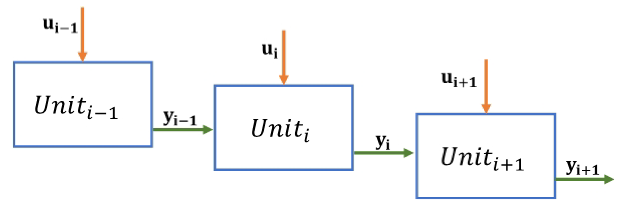
Industrial chemical plants are made up of interconnected units. Changes in the feed stream make the outputs of a unit fluctuate and disturb the units downstream. Thus, the connections between processing units that share streams mean losing degrees of freedom. The nature and source of input disturbances in these systems are varied. These can be small and slow fluctuations, such as alterations in environmental conditions. At other times, imperceptible changes degrade the plant performance gradually, for instance, due to equipment fouling. Then, random or periodic fluctuations in pressure, flow, or temperature in the fed streams occur, for example, by transients in the auxiliary services. Such disturbances yield inputs with a type of behavior that can be represented by a sum of periodic signals and can be treated as signals falling within a reduced frequency range. Otherwise, sharp and severe changes may occur due to unexpected operation of the plant in unstable or critically stable regions. Reference changes represent alike substantial transition. The inputs are abrupt and also within a narrow frequency band in the last two examples. The disturbance model accompanying the control design proposed here integrates a Dirac pulse as excitation. As a result, we ensure that this type of disturbance can be shaped. In a broad sense, the disturbances are endogenous and exogenous. The first class consists of unmeasured, uncertain, or unknown internal dynamics. The second class includes external sources, such as environmental changes and unit interactions. The control law synthesis can deal with several performance specs, but one of the main features is to assess its potential for disturbance rejection. In a closed-loop simulation, the described disturbances are input signals, such as positive or negative small-amplitude steps, slow ramp-type changes, or oscillations built up by weighted sums of sinusoidal signals of varied frequencies in short intervals. These input changes can be continuous or shift with different time spans and may co-occur. The parametric uncertainty and the non-modeled phenomena can be accounted for as disturbances. However, the closed-loop system can cope with these other dynamics because the controller is based on a robust design that meets the robustness margins.

An overview of the literature on process control is given with a focus on disturbance rejection schemes. One of the most practiced approaches to address this problem is the active disturbance rejection control (ADRC). This technique’s core is the real-time estimation of a generalized disturbance that couples transients induced by endogenous and exogenous disturbances [1,2,3,4]. As the PID control, the ADRC is an error-driven control scheme rather than a model-driven scheme. It uses extended state observers (ESO) to estimate the global disturbance online. The generalized disturbance is assumed to be unstructured and depends on input and output signals in an unknown way. Then, the feedback control action achieves the rejection of the generalized disturbance. A review of the main features of the ADRC technique is given in [5,6].

The ADRC, thought initially for nonlinear systems, needs nonlinear ESOs and addressing other common issues in studying nonlinear systems. Gao [7] and later [8] introduced the linear active disturbance rejection control (LADRC) for controller scaling of a larger plant class. It is based on a simple parameterization with linear gains bandwidth tuning. For simplicity, the same bandwidth is rated for both the observer and control; the larger the bandwidth, the better the rejection of disturbances. The linear approach makes it easier to analyze system stability and frequency response compared to the nonlinear one. With a different perspective, Liu et al. [9] proposed to obtain model information in a frequency-based LADRC. This last scheme was proved to control a complex chemical process with two structures; only one receives online information from a system model. As a result, the LADRC with the model knowledge had a faster response, better overall performance, and a greater capacity to reject disturbances. Meng et al. [10] implemented in a four-tank system both non-linear and linear ADRC schemes, calling it L/ADRC, and obtained as a result an observation and compensation of the disturbance, as well as the transition process for reference input and achieved good position control.

With a distinct approach, Wang et al. [11] extended the ADRC structure into an internal model control (IMC) framework. This theory lies on the standard open-loop frequency-domain analysis. Lastly, the ADRC control performance grows by tuning an integral gain. At the same time, Carreno-Zagarra et al. [12] proposed a scheme that meets the PI control and the linear ADRC. It uses generalized proportional–integral (GPI) observers, an ESO class. This scheme was used to obtain a robust output feedback control to regulate the pH in a photobioreactor. Wei et al. [13] deduced that a PD controller is not good enough to eliminate disturbances and, besides, the pure high-order integrator is challenging to stabilize. Instead, they proposed to obtain a robust control for the active disturbance rejection of the U model (explained as the conversion in the closed-loop of a plant to be G(s) = y(s)/u(s) = 1, by designing a control law based on an inverse model of the plant). The desired closed-loop behavior is fixed to deal with the system needs. The scheme integrates the control of the U model and the Glover–McFarlane control (a control design that resolves system performance and robustness). A newer algorithm was given by Ren et al. [14]. In this strategy, the PD in the ADRC was replaced with a proportional integral type generalized predictive control (PI-GPC) to track the reference and reject disturbances. This scheme was applied to control a distillation column with a long delay. Further research works where the ADCR is used were reported by Buche et al. [15,16], who used an adaptive disturbance compensation filter to handle significant plant modeling uncertainties. According to the survey, for chemical processes, the ADCR is one of the control schemes most widely used for disturbance rejection.

A related approach also uses observers to estimate a global disturbance. It was proposed by An et al., 2016 [17]. They designed a disturbance observer-based anti-windup feedback control scheme. The control objective was to regulate velocity and altitude in an air-breathing hypersonic vehicle with input saturation. The control challenge was to model the global or lumped disturbance, which, like the ADRC approach, carries the overall influence of potential uncertainties and disturbances. The control scheme addressed stability robustness and steady-state error. Then, the control performance was enhanced by considering an anti-windup property to deal with input constraints. As a result, the reference tracking was achieved with smooth control inputs.

Adaptive regulation is another of the most recognized strategies for disturbance rejection. In this case, typical applications are for mechanical, electrical, and electromechanical systems. The adaptive scheme leads to an asymptotic attenuation of the effects due to unknown or time-varying disturbances. One specifies a dynamic model of these in the closed-loop system as the primary measure to settle the problem. In this scheme, the internal model principle (IMP) aids in performing an indirect adaptive control as done by Chen and Tomizuka [18]. Once a disturbance model is met, the parameters can be tuned. Hu and Pota [19] estimated a narrow-band noise perturbation via the IMP. They then devised a disturbance observer (DOB) using a band-pass filter with multiple narrow bands. The resulting perturbation model gives robust stabilization for the convergent parameters. Wang et al. [20] used the IMP to solve the issue of trajectory tracking coupled with perturbation rejection in random systems. This control with mixed feedforward and feedback structure was conceived by assigning poles to form an augmented system. The tunable parameters made the following error small and the random system stable.

Youla–Kucera parameterization enables the entry of the internal model of disturbance into the controller by updating the parameters of the Q polynomial (YK filter). In the presence of unknown disturbances, it is likely to build a direct control scheme where the parameters of Q are set so that we do not need to calculate the controller further. The estimation of the polynomial Q is subject to the denominator of the perturbation model [21]. A close algorithm for direct adaptive regulation was presented by Valentinotti et al. [22]. Their technique was well suited for rejecting unstable perturbations in batch fermentation with Saccharomyces cervisiae. The operational objective was to maximize biomass production while keeping the substrate concentration at a critical point in the reactor. As a result, the control law kept constant the ethanol concentration. On the other hand, the substrate cell’s consumption was modeled as an exponential growing perturbation that the control was intended to cancel. A direct adaptive control law was computed based on linear models, YK parameterization, and the IMP. It is worthy to note that this method needs to estimate the Q polynomial online (for the study case, only one parameter has been estimated, which specifies the cell growth rate).

We found that the outlined adaptive control strategy for disturbance rejection has already been tested in different systems. However, we mainly revisited control techniques for systems exposed to narrow-band disturbances. In this context, we refer first to the control problem of an active suspension. Prepared for this system, Landau [23] launched a benchmark to treat multiple unknown perturbations in a small range of frequencies, assumed along with time variants. The challenge was attenuating one, two, and three sinusoidal disturbances in the range of 50 to 95 Hz. The control objective was to obtain an attenuation of 40 dB. The controllers submitted to the benchmark used models from a YK factorization with a proper choice of polynomials. Then, a feedback structure produced perturbation attenuation (at least asymptotically) through an adaptive approach that accounts for a model of unknown perturbations. Airimi et al. [24], and Castellanos Silva et al. [25] illustrated direct adaptive regulation schemes that couple YK and IMP parameterization. Castellanos Silva et al. [25] made a thorough selection of the assigned closed-loop poles for computing a central controller. Later, Castellanos et al. [26] suggested an ameliorated scheme involving an adaptive Youla–Kučera IIR filter, called the $\rho$-notch structure (i.e., the poles of the disturbance model are roots on the unit circle). Another proposal to deal with narrow-band disturbances was for noise cancellation in an acoustic duct. In [27], a control scheme founded on the YKP and IMP worked out this issue. The experiment involved exciting the loudspeaker with a single sinusoidal signal tone and running the adaptive controller to cancel the noise in a high-performance microphone. This control scheme performed well for the presumed narrow range of frequencies.

Still, on the same topic, Landau et al. [28] carried out practical research on damping multiple narrow-band disturbances. At this time, the work cared for different frequency regions. The idea was to quantify the interference arising when leading with close frequencies. A robust control was the preferred technique, which used the knowledge of how the disturbance frequencies vary. Then, a direct adaptive control algorithm also grounded on the IMP, and the YK parameterization improved the basic control scheme. As a result, the control law faced multiple disturbances better. Other research works about noise damping in an acoustic duct are those by Landau and Meléndez [29], Landau et al. [30] and Airimitoaie et al. [31]. These imply two adaptive designs commonly built for active noise compensation and viewed as vibration control. The first was with an FIR compensator structure, and the second was YK parameterization of the feedforward noise compensator. The second approach of [31] allows to contrast two points: stabilize the internal positive feedback loop and attenuate the residual noise. Vau and Landau [32] developed a controller with dual YK parameterization for the adaptation of controller parameters to deal with modeling uncertainties; this methodology was tested in simulations and and implemented in an active noise control system.

There are other relevant adaptive control approaches, whose designs introduce different features and performance that could eventually be extrapolated to process applications. The following research is described as an example. An adaptive control was proposed for the electric system, but at this time, observers perform the disturbance estimate. It was reported by Shen et al., 2021 [33], who synthesized an adaptive second-order sliding mode control. The scheme was conceived with a twofold objective: to regulate the voltage in a three-level neutral-point-clamped converter and to track the instantaneous power. The nonlinear system was subject to parameter variation and external disturbances. Then, a switched high-gain observer was used to estimate the disturbance. In contrast to a classic observer design, the new one reduced the performance degradation caused by measurement noise. A distinctive feature of this approach is that the control scheme does not need knowledge of the disturbance boundaries as it usually is. Adaptive control has also been combined with neural network-based structures. Wu et al., 2017 [34], presented a fuzzy adaptive feedback control for networked control systems (NCSs). The NCSs use digital communication networks to distribute their components in different geographical locations rather than point-to-point communication. Their scheme reached unknown nonlinear behavior in SISO NCSs. The challenge was to deal with intermittent and stochastic data loss in the transmission process, which was inferred as a delay in the controller design. A Pade approximation dealt with the delay. This fuzzy adaptive scheme preserved stability and the desired closed-loop behavior in nonlinear and delayed systems with data loss.

In what follows, the search is more focused on our physical system. An operating CSTR may move away from the nominal region due to interactions between variables, interchanges with other units, disturbances, or properties changing over time. These perturbations accentuate the impact of the plant’s nonlinearities and natural frequencies on the outputs and stability of the system. It is worth noting that classical linear control is insufficient for the regulation and tracking tasks in CSTR systems ([35]). As a result, a wide range of advanced control techniques has been reported to address a number of challenges imposed by the inherent complex behaviors in CSTR. The literature in this field is extensive. In a broad sense, one of the most applied techniques has been robust control. It handles nonlinearities, uncertainty, interactions, and disturbances via coupled or decoupled schemes. As an example, we cite the work of Prokop et al., 2019 [35]. They designed a 2-degrees-of-freedom compensator with feedback and feedforward parts. Their control objective was to regulate and track an uncertain CSTR. Their control synthesis needed an uncertain linear model, including a family of all feasible plants modeled by the ring of stable rational functions. A robust stability analysis was stated through a graphical method. The method used the value set concept and the zero exclusion condition. Then, an algebraic approach led to a Diophantine equation, which was solved to obtain all stabilizing feedback controllers dealing with disturbance rejection. A second Diophantine equation gave the condition for reference tracking.

There are many robust approaches. We cite another work testing and improving one of them. Li et al., 2021 [36], studied a sliding control enhanced with an event-triggered approach. The given asynchronous strategy regulated a CSTR subject to temperature fluctuations. A Markov model described the perturbed system by replicating a multi-mode switching behavior. Then, an asynchronous state observer estimated the unmeasured states. In order to resolve whether the current data should be released in the switching mode, an event-triggered approach dealt with packet loss, transmission delay, and random disturbance. As an outcome, the control law reduced computation effort. The controller was built to gain stability and finite time reachability of the sliding dynamics. Then, introducing an adaptive part in a robust control is also an effective practice. In [37], two neural networks (NNs)-based robust adaptive controllers were designed to face input nonlinearities and unknown disturbances in CSTRs. The first NN overcame an unknown input dead zone, whereas the second treated the issue of actuator saturation.

One way to approach the control of a nonlinear system is through global transformations to move from the original nonlinear model to an exact linear model with a different set of variables. In [38], an adaptive scheme with intelligent control is given for an uncertain CSTR. This work tested two transformations in a robust control for some duties. Other standard and advanced techniques can be improved indeed by modern optimization methods. Khanduja and Bhushan, 2019 [39], submitted a hybrid control for a CSTR which offers a stable convergence. A PID was improved by the tuning procedure based on firefly and biogeography optimization.

In this paper, we assumed that the disturbances into the system fall within a narrow band of frequencies. Thus, we adapted the earlier mapped control structure based on the disturbance model to control a chemical plant effectively. In summary, this paper addresses disturbance rejection in three continuous stirred tank reactors linked in series by adaptive control. In contrast to similar controllers for other types of systems, our approach characterizes the input and output disturbances as signals in a narrow frequency band. We looked for a twofold objective, regulation of the operating point and disturbance rejection. Our scheme consists of a robust RST control enhanced by the YK filter and the IMP. The design follows the dynamics of unknown perturbations that continuously alter the input and output of the plant. We synthesized an adaptive control scheme. Later on, we assessed its performance for different sorts of disturbances. As an outcome, we demonstrated that the control law guarantees the disturbances rejection. A better performance was observed in contrast with that obtained by an MPC, a well-established control technique.

The remainder of this paper is organized as follows. Section 2 introduces the plant and the temperature sensor model. In Section 3, the adaptive controller design is explained. Section 4 describes the control synthesis of the temperature control. In Section 5, the controller performance trials are given. Finally, we conclude in Section 6.

2. Plant Description

An irreversible exothermic first-order reaction $A\stackrel{k}{\to }B$ occurs in three continuous stirred tank reactors (CSTR) connected in series. The feed stream ($F_{R_{in},1}$, $T_{R_{in},1}$ and $C_{A_{in},1}$) enters $R_1$, and the flow moving out of $R_3$ ($C_{A,3}$, $T_{R,3}$ and $F_{R,3}$) carries the process product. A cooling jacket surrounds each CSTR to remove the heat produced by the reaction. The cooling fluid fed at $T_{J_{in},i}$ (with i the unit number) circulates in the jacket with a volumetric flow $F_{J,i}$. A diagram of the system is shown in Figure 1, and Figure 2 shows relationships of the system variables for the three CSTR reactors in series as they are within the controller.

To operate the units in series is a common form of process intensification because the total volume of the reactors can be efficiently reduced. Moreover, to look for homogeneity of temperature, concentration, and liquid properties in the reactors results in being more manageable. On the other hand, interactions between units are indeed settled. It means that disturbances in one process unit influence the dynamics of the subsequent. The ongoing reaction can lead the configuration in series to unstable operation. These issues lead to a further challenging control problem as opposed to the single-reactor control problem. From a control point of view, the three reactors can be represented in Figure 2, where $u_i$ is the manipulated variable and $y_i$ represents the flow output of unit i. The output of unit i is the input of unit $i+1$.

2.1. Non-Linear Model

The behavior of an CSTR is dictated by the conservation equations derived for the reactor and the cooling jacket under the assumptions of perfect mixing, negligible heat losses, constant volume of the reactor (i.e., ideal level control), and non-isothermal operation. The model of unit i ($i=1,\dots ,N_u$, where $N_u$ is the number of units) is a set of three nonlinear differential equations that reproduce the dynamic evolution of the concentration of the reactant A, $C_{A,i}$ and the temperatures of the reactor $T_{R,i}$ and the cooling jacket $T_{J,i}$. The global process is represented by a 9th order model (1). A study of the equilibrium states and static stability predicted by the non-linear model, mainly for $R1$ is given in the next section for the numerical example outlined in that part. The idea is to give insight into the control challenges.

$$\begin{array}{cccc}\mathrm{Global}\mathrm{material}\mathrm{balance}\hfill & F_{R,i}\hfill & =\hfill & F_{R_{in},i}\hfill \\ \hfill & \hfill & \\ \mathrm{Component}\mathrm{material}\mathrm{balance}\hfill & \frac{d{C}_{A,i}}{dt}\hfill & =\hfill & \frac{F_{R,i}}{V_{R,i}}\left(C_{A_{in},i}-C_{A,i}\right)-k_i{C}_{A,i}\hfill \\ \hfill & \hfill & \\ \mathrm{Energy}\mathrm{balance}\mathrm{in}\mathrm{the}\mathrm{reactor}\hfill & \frac{d{T}_{R,i}}{dt}\hfill & =\hfill & \frac{F_{R,i}}{V_{R,i}}\left(T_{R_{in},i}-T_{R,i}\right)-\frac{\lambda k_i{C}_{A,i}}{{\rho }_R{C}_{P_R}}-\frac{U{A}_{H,i}}{{\rho }_R{C}_{P_R}{V}_{R,i}}\left(T_{R,i}-T_{J,i}\right)\hfill \\ \hfill & \hfill & \\ \mathrm{Energy}\mathrm{balance}\mathrm{in}\mathrm{the}\mathrm{cooling}\mathrm{jacket}\hfill & \frac{d{T}_{J_i}}{dt}\hfill & =\hfill & \frac{F_{J_i}}{V_{J,i}}\left(T_{J_{in},i}-T_{J,i}\right)+\frac{U{A}_H}{{\rho }_J{C}_{P_J}{V}_{J,i}}(T_{R,i}-T_{J,i})\hfill \\ \hfill & \hfill & \\ \mathrm{Kinetic}\mathrm{equilibrium}\left(\mathrm{Arrhenius}\mathrm{equation}\right)\hfill & k_i\hfill & =\hfill & \alpha {exp}^{\frac{-E_A}{R_g{T}_{R,i}}}\hfill \end{array}$$

(1)

In the standard form, the nonlinear model becomes

$$\begin{array}{ccc}\hfill {\dot{\mathbf{x}}}_i& =& {\mathcal{A}}_i\left({\mathbf{u}}_i,{\mathbf{k}}_i\left({\mathbf{x}}_i\right)\right){\mathbf{x}}_i+{\mathcal{B}}_i\left({\mathbf{u}}_i\right){\mathbf{u}}_i\hfill \end{array}$$

(2)

$$\begin{array}{ccc}\hfill {\mathbf{y}}_i& =& {\mathcal{C}}_i{\mathbf{x}}_i\hfill \end{array}$$

(3)

The states (${\mathbf{x}}_i$), inputs (${\mathbf{u}}_i$), and outputs (${\mathbf{y}}_i$) for each unit of the serial process are given as follows:

$${\dot{\mathbf{x}}}_i=\left[\begin{array}{c}{\dot{x}}_{i,j}\end{array}\right]=\left[\begin{array}{c}{\dot{x}}_{i,1}\\ {\dot{x}}_{i,2}\\ {\dot{x}}_{i,3}\end{array}\right]=\left[\begin{array}{c}\frac{d{C}_{A,i}}{dt}\\ \frac{d{T}_{R,i}}{dt}\\ \frac{d{T}_{J,i}}{dt}\end{array}\right],{\mathbf{u}}_i=\left[\begin{array}{c}{u}_{i,j}\end{array}\right]=\left[\begin{array}{c}{u}_{i,1}\\ u_{i,2}\\ u_{i,3}\\ u_{i,4}\\ u_{i,5}\end{array}\right]=\left[\begin{array}{c}{F}_{R_{in},i}\\ C_{A_{in},i}\\ T_{R_{in,i}}\\ T_{J_{in},i}\\ F_{J,i}\end{array}\right],{\mathbf{y}}_i=\left[\begin{array}{c}{y}_{i,j}\end{array}\right]=\left[\begin{array}{c}{y}_{i,1}\\ y_{i,2}\end{array}\right]=\left[\begin{array}{c}{C}_{A,i}\\ T_{R,i}\end{array}\right],{\mathbf{k}}_i=\left[\begin{array}{c}\alpha {exp}^{-\frac{E_A}{R_g{x}_{i,2}}}\end{array}\right]$$

(4)

The subscripts i and j stand for the unit process and the vector component, respectively. The matrices ${\mathcal{A}}_i$, ${\mathcal{B}}_i$, and ${\mathcal{C}}_i$ of the nonlinear system are given in Appendix A.1.

2.2. Linear Model

We linearize Equations (2) and (3) around an operating point. From now on, we distinguish between input variables (${\mathbf{u}}_i$) and disturbances (${\mathbf{d}}_i$).

$$\frac{d{\mathbf{x}}_{\mathrm{dv},i}}{dt}={\mathbf{A}}_i{\mathbf{x}}_{\mathrm{dv},i}+{\mathbf{B}}_i{\mathbf{u}}_{\mathrm{dv},i}+{\mathbf{E}}_i{\mathbf{d}}_{\mathrm{dv},i}i=1,2,3.$$

(5)

where ${\mathbf{A}}_i$, ${\mathbf{B}}_i$, and ${\mathbf{E}}_i$ are Jacobian matrices evaluated at the nominal operating point. The model is expressed in terms of deviation variables, denoted by the subscript $dv$.

$${\mathbf{x}}_{\mathrm{dv},i}=\left[\begin{array}{c}{x}_{i,j}-x_{i,j,ss}\end{array}\right]=\left[\begin{array}{c}{x}_{dv,i,1}\\ x_{dv,i,2}\\ x_{dv,i,3}\end{array}\right]=\left[\begin{array}{c}{C}_{A,i}-C_{A,i,ss}\\ T_{R,i}-T_{R,i,ss}\\ T_{J,i}-T_{J,i,ss}\end{array}\right],{\mathbf{u}}_{\mathrm{dv},i}=\left[\begin{array}{c}{u}_i-u_{i,ss}\end{array}\right]=\left[\begin{array}{c}{F}_{J,i}-F_{J,i,ss}\end{array}\right],$$

$${\mathbf{y}}_{\mathrm{dv},i}=\left[\begin{array}{c}{y}_i-y_{i,ss}\end{array}\right]=\left[\begin{array}{c}{T}_{R,i}-T_{R,i,ss}\end{array}\right],\mathrm{and}{\mathbf{d}}_{\mathrm{dv},i}=\left[\begin{array}{c}{d}_{i,j}-d_{i,j,ss}\end{array}\right]=\left[\begin{array}{c}{F}_{R,i}-F_{R,i,ss}\\ T_{J_{in},i}-T_{J_{in},i,ss}\end{array}\right].$$

(6)

The subscript $ss$ denotes steady-state variables, ${\mathbf{u}}_{\mathrm{dv},i}\in {\Re }^{m_1}$ is the vector of $m_1$ input variables, and ${\mathbf{d}}_{\mathrm{dv},i}\in {\Re }^{m_2}$ is the vector of $m_2$ disturbances variables, ${\mathbf{x}}_{\mathrm{dv},i}\in {\Re }^n$ is the vector of n state deviation variables (${\mathbf{x}}_{\mathrm{dv},i}=x_i-x_{i,ss}$ for $i=1,2,3$), and ${\mathbf{y}}_{\mathrm{dv},i}\in {\Re }^r$ is the vector of r output variables.

$${\mathbf{A}}_{i,j}=\frac{\partial f_i}{\partial x_j}{|}_{x_{dv,i}},{\mathbf{B}}_i=\frac{\partial f_i}{\partial u_i}{|}_{u_{dv,i}},{\mathbf{C}}_i=\frac{\partial f_i}{\partial x_i}{|}_{y_{dv,i}},{\mathbf{E}}_i=\frac{\partial f_i}{\partial d_i}{|}_{d_{dv,i}}$$

with $i=1,2,3$ (process unit) and j elements in the states vector. The matrices elements of the linear system ${\mathbf{A}}_i$, ${\mathbf{B}}_i$, and ${\mathbf{E}}_i$ are given explicitly in Appendix A.2.

Applying the Laplace transformation and recursively inserting variables of the upstream process unit, the transfer function of the system becomes

$$\mathbf{y}\left(s\right)=\mathbf{G}\left(s\right)u\left(s\right)+{\mathbf{G}}_d\left(s\right)\mathbf{d}\left(s\right)$$

(7)

where $\mathbf{y}\left(s\right)$ is the output vector, $\mathbf{u}\left(s\right)$ is the input vector, $\mathbf{d}\left(s\right)$ is the disturbance vector, and ${\mathbf{M}}_i={(sI-{\mathbf{A}}_{i,i})}^{-1}$.

$$\mathbf{G}\left(s\right)=\left[\begin{array}{ccc}{\mathbf{C}}_1{\mathbf{M}}_1{\mathbf{B}}_1& 0& 0\\ {\mathbf{C}}_2{\mathbf{M}}_2{A}_{2,1}{\mathbf{M}}_1{\mathbf{B}}_1& {\mathbf{C}}_2{\mathbf{M}}_2{\mathbf{B}}_2& 0\\ {\mathbf{C}}_3{\mathbf{M}}_3{A}_{3,2}{\mathbf{M}}_2{A}_{2,1}{\mathbf{M}}_1{\mathbf{B}}_1& {\mathbf{C}}_3{\mathbf{M}}_3{A}_{3,2}{\mathbf{M}}_2{\mathbf{B}}_2& {\mathbf{C}}_3{\mathbf{M}}_3{\mathbf{B}}_3\end{array}\right]=\left[\begin{array}{ccc}{\mathbf{G}}_{1,1}& 0& 0\\ {\mathbf{G}}_{2,1}& {\mathbf{G}}_{2,2}& 0\\ {\mathbf{G}}_{3,1}& {\mathbf{G}}_{3,2}& {\mathbf{G}}_{3,3}\end{array}\right].$$

(8)

The transfer function of the multivariable process is a triangular matrix. Thus, the response of a unit is influenced by the output of the previous one. However, a decoupled design of the control law is proposed here, and the interaction between the process units is assumed as a disturbance.

2.3. Temperature Sensor Simulation

We use the standard polynomial parameterization defined by the NIST ITS-90 Thermocouple Database [40] to reproduce the behavior of a thermocouple type S. The model determines the voltage across the device as a function of the temperature. This empirical equation is used along with Newton’s Equation (9) which describes the heat flow into the sensor, assuming the sensor as a finite mass with uniform temperature distribution. The simulation of the temperature sensor dynamics dictates the thermal behavior depending on the dissipation factor and the thermal time constant, and produces a small noise in the measurement of the output of the system, i.e., the reactor temperature $T_R$. For a constant temperature recording, Figure 3 shows the noisy measured signal in an open-loop simulation. The response is a signal oscillating in time with an amplitude of 0.3 K below the nominal temperature value. Since Newton’s equation is a first-order differential equation, the dynamic behavior of the sensor is also a disturbance occurring with a reduced frequency range. This signal has evidently a small amplitude with respect to the measured value and is inserted to the controller block in the closed-loop simulations.

$$Q_{T_R}=K_d{t}_c\frac{d{T}_{R,i}}{dt}$$

(9)

where $T_R$ is the temperature at port A on the thermocouple. $Q_{T_R}$ is the net heat flow to port A. $K_d$ is the value of the dissipation factor parameter. $t_c$ is the value of the thermal time constant parameter. $d{T}_R/dt$ is the rate of change of temperature.

3. Control Design

The control objective is to regulate the output composition of a disturbed and uncertain process of three CSTR in series. The goal is to keep an isothermal operation while the reaction conversion holds the nominal condition. Figure 4 shows the proposed global control scheme. The design deals with the fulfillment of the operating conditions specs by a central RS-type polynomial control law (red dashed line in Figure 4). Besides, to deal with disturbances and uncertainty at the input and output of the tanks, the control law integrates adaptive control (red line in Figure 4). The adaptive frame consists of a disturbance model, delivered in the form of a Youla–Kučera filter or Q filter, and a suitable algorithm for online parameter adaptation. Q is given as a polynomial, then added to the control scheme without effect on the performance of the central RS controller. From the design point of view, the disturbances are modeled via a known structure since a specific class of input changes is wielded. A known structure with unknown parameters is then assumed to describe the disturbance transfer function. The disturbance signal is produced by a Dirac pulse filtered with a deterministic model (disturbance transfer function). In this way, the principle of the internal model makes disturbance rejection possible [21,41,42].

The strategy to update the control law is to estimate the filter Q online. An observation vector of the disturbance is built from the measured input-output data of the plant, the filter Q being a function of $w\left(t\right)$ (Figure 4) and the chosen closed-loop poles and zeros. The structure is equivalent to a FIR filter. The adaptive control loop is based on the least mean square of the error computation and allows recalculating the polynomial $S\left(q^{-1}\right)$. Hence, the disturbance rejection is asymptotically attained [29,30].

In this section dedicated to the control design, we used the delay operator $q^{-1}$ for describing the system’s behavior in the time domain. In the next section, we describe the numerical simulation with the complex variable $z^{-1}$ for characterizing the system’s behavior in the frequency domain.

3.1. Central RS Controller

The control structure to be implemented is the local loop control, where the inputs of a unit are used to control the outputs of the same unit. The central RS controller is a polynomial controller, designed by pole placement. For three CSTR reactors connected in series, the transfer function in closed loop with local control is given by

$$\begin{array}{ccc}\hfill \mathbf{L}& =& \left[\begin{array}{ccc}{G}_{1,1}\left(q^{-1}\right)& 0& 0\\ G_{2,1}\left(q^{-1}\right)& G_{2,2}\left(q^{-1}\right)& 0\\ G_{3,1}\left(q^{-1}\right)& G_{3,2}\left(q^{-1}\right)& G_{3,3}\left(q^{-1}\right)\end{array}\right]\left[\begin{array}{ccc}{K}_{1,1}\left(q^{-1}\right)& 0& 0\\ 0& K_{2,2}\left(q^{-1}\right)& 0\\ 0& 0& K_{3,3}\left(q^{-1}\right)\end{array}\right]\hfill \\ & =& \left[\begin{array}{ccc}{G}_{1,1}\left(q^{-1}\right)K_{1,1}\left(q^{-1}\right)& 0& 0\\ 0& G_{2,2}\left(q^{-1}\right)K_{2,2\left(q^{-1}\right)}& 0\\ 0& 0& G_{3,3}\left(q^{-1}\right)K_{3,3}\left(q^{-1}\right)\end{array}\right]\hfill \end{array}$$

(10)

To obtain Equation (10), the model was linearized around an operating point by the standard approach of the Taylor’s series expansion and the knowledge of the Jacobian linearization process. Then, the Laplace transform was applied. As a serial process, it is split into sub-processes that we call units, where the states depend on the states in the same unit and the states of the previous one. Hence, the shape of the transfer matrix is a lower diagonal. For the case of simple control loops, the feedback gain is a diagonal matrix because each control affects only the unit where it is applied. For more details, see [43]. To deal with the rejection of exogenous disturbances, an adaptive block is added to the RS controller. An adaptive control as shown in Figure 4 is synthesized for each reactor (local loop control structure $u_i=K_{i,i}\left(q^{-1}\right)y_i$).

RS Robust Control

The RS robust control synthesis is obtained from the linear model of the plant in discrete time, given in (11)

$$G_{i,i}\left(q^{-1}\right)=\frac{q^{-d}B\left(q^{-1}\right)}{A\left(q^{-1}\right)}$$

(11)

where

$$\begin{array}{ccc}\hfill A\left(q^{-1}\right)& =& 1+a_1{q}^{-1}+\cdots +a_{n_A}{q}^{-n_A}\hfill \end{array}$$

(12)

$$\begin{array}{ccc}\hfill B\left(q^{-1}\right)& =& b_1{q}^{-1}+\cdots +b_{n_B}{q}^{-n_B}=q^{-1}{B}^{*}\hfill \end{array}$$

(13)

$$\begin{array}{ccc}\hfill B^{*}\left(q^{-1}\right)& =& b_1+\cdots +b_{n_B}{q}^{-n_B+1}\hfill \end{array}$$

(14)

where d is the plant time delay given as the number of sampling periods, $A\left(q^{-1}\right)$, $B\left(q^{-1}\right)$, $B^{*}\left(q^{-1}\right)$ are polynomials in the complex variable $q^{-1}$, $n_A$, $n_B$, and $n_B-1$ represent their orders. The controller $K_{i,i}$ is expressed in (15), in terms of $R\left(q^{-1}\right)$ and $S\left(q^{-1}\right)$.

$$K_{i,i}\left(q^{-1}\right)=\frac{R\left(q^{-1}\right)}{S\left(q^{-1}\right)}=\frac{r_0+r_1{q}^{-1}+\cdots +r_{n_R}{q}^{-n_R}}{1+s_1{q}^{-1}+\cdots +s_{n_S}{q}^{-n_S}}$$

(15)

The output $y\left(t\right)$ and the input $u\left(t\right)$ of the plant are, respectively,

$$\begin{array}{ccc}\hfill y\left(t\right)& =& \frac{q^{-d}B\left(q^{-1}\right)}{A\left(q^{-1}\right)}u\left(t\right)+\frac{q^{-d}B\left(q^{-1}\right)}{A\left(q^{-1}\right)}v\left(t\right)\hfill \end{array}$$

(16)

$$\begin{array}{ccc}\hfill S\left(q^{-1}\right)u\left(t\right)& =& -R\left(q^{-1}\right)y\left(t\right)\hfill \end{array}$$

(17)

where $v\left(t\right)$ is the resulting additive disturbance on the input of the system, $R\left(q^{-1}\right),S\left(q^{-1}\right)$ are polynomials in $q^{-1}$ with orders $n_R,n_S$

$$\begin{array}{ccc}\hfill R\left(q^{-1}\right)& =& r_0+r_1{q}^{-1}+\cdots +r_{n_R}{q}^{-n_R}\hfill \\ & =& R^{\prime }\left(q^{-1}\right)H_R\left(q^{-1}\right)\hfill \end{array}$$

(18)

$$\begin{array}{ccc}\hfill S\left(q^{-1}\right)& =& 1+s_1{q}^{-1}+\cdots +s_{n_S}{q}^{-n_S}\hfill \\ & =& S^{\prime }\left(q^{-1}\right)H_S\left(q^{-1}\right)\hfill \end{array}$$

(19)

where $H_R\left(q^{-1}\right)$ and $H_S\left(q^{-1}\right)$ are pre-specified and fixed parts of the controller that perform tasks such as rejecting disturbances, reducing the steady-state error ($H_S\left(q^{-1}\right)$) or opening the loop ($H_R\left(q^{-1}\right)$). The $R\left(q^{-1}\right)$ and $S\left(q^{-1}\right)$ polynomials of the control law are obtained by specifying the desired performance. The procedure is to select the closed-loop poles to generate the Bézout identity associated with the control problem. The Bézout identity gives the closed-loop poles in the form of $P\left(q^{-1}\right)$ and is written as indicated by (20), as a function of the polynomials $R\left(q^{-1}\right)$, $S\left(q^{-1}\right)$, and the open-loop plant model given by a $A\left(q^{-1}\right)$ and $B\left(q^{-1}\right)$, then it is solved for each process unit.

$$P\left(q^{-1}\right)=A\left(q^{-1}\right)S\left(q^{-1}\right)+B\left(q^{-1}\right)R\left(q^{-1}\right)$$

(20)

After pole assignment, to ensure general robustness, the design of the controller is achieved by shaping the sensitivity functions of the closed-loop system. In our design, robustness is obtained by managing both the delay margin and the modulus margin. The sensitivity functions are transfer functions that relate disturbances to the system output $S_{yp}$ as in (21) or input $S_{up}$ as in (22). The setting of the sensitivity functions $S_{yp}$ and $S_{up}$ must be performed within the allowed values of the margins [44].

$$S_{yp}\left(q^{-1}\right)=\frac{A\left(q^{-1}\right)S\left(q^{-1}\right)}{A\left(q^{-1}\right)S\left(q^{-1}\right)+B\left(q^{-1}\right)R\left(q^{-1}\right)}$$

(21)

$$S_{up}\left(q^{-1}\right)=\frac{-A\left(q^{-1}\right)R\left(q^{-1}\right)}{A\left(q^{-1}\right)S\left(q^{-1}\right)+B\left(q^{-1}\right)R\left(q^{-1}\right)}$$

(22)

For a disturbance in the plant input signal, the input–output disturbance sensitivity function is the transfer function that accounts for the effect of the input disturbance $v\left(t\right)$ on the system output. It is written as

$$S_{yv}\left(q^{-1}\right)=\frac{B\left(q^{-1}\right)S\left(q^{-1}\right)}{A\left(q^{-1}\right)S\left(q^{-1}\right)+B\left(q^{-1}\right)R\left(q^{-1}\right)}$$

(23)

3.2. Adaptive Scheme for Input and Output Disturbances Rejection

A practical approach to mitigate the effect of disturbances is to introduce the disturbance dynamics into the closed-loop system. This update is performed by applying the internal model principle [41,45].

3.2.1. Internal Model Principle

The effect of the input disturbance ($v\left(t\right)$) on the output is written as

$$y\left(t\right)=\frac{B\left(q^{-1}\right)S\left(q^{-1}\right)}{P\left(q^{-1}\right)}v\left(t\right)=S_{yv}\left(q^{-1}\right)v\left(t\right)$$

(24)

We assume that the disturbance $v\left(t\right)$ is modeled as a signal passing through a filter and is modeled by

$$v\left(t\right)=\frac{N_p\left(q^{-1}\right)}{D_p\left(q^{-1}\right)}\delta \left(t\right)$$

(25)

where $\delta \left(t\right)$ is a Dirac impulse, $N_P\left(q^{-1}\right)$ and $D_p\left(q^{-1}\right)$ are coprime polynomials, and $n_{N_P},n_{D_P}$ represent the order. This approach has been used in [32,46,47,48]. $P\left(q^{-1}\right)$ is an asymptotically stable polynomial, converges asymptotically towards zero if and only if the polynomial $S\left(q^{-1}\right)$ in the $RS$ control has the form

$$S\left(q^{-1}\right)=D_p\left(q^{-1}\right)S^{\prime }\left(q^{-1}\right)$$

(26)

$$H_S\left(q^{-1}\right)=D_p\left(q^{-1}\right)$$

This way, it becomes feasible to include disturbances in the control loop and then reject them.

3.2.2. Youla–Kučera (YK) Parameterization

Using YK parameterization or Q parameterization, the controller polynomials $R\left(q^{-1}\right)$ and $S\left(q^{-1}\right)$ obtain the form

$$\begin{array}{ccc}\hfill R\left(q^{-1}\right)& =& R_0\left(q^{-1}\right)+A\left(q^{-1}\right)Q\left(q^{-1}\right)\hfill \end{array}$$

(27)

$$\begin{array}{ccc}\hfill S\left(q^{-1}\right)& =& S_0\left(q^{-1}\right)-q^{-d}B\left(q^{-1}\right)Q\left(q^{-1}\right)\hfill \end{array}$$

(28)

The central controller $R_0\left(q^{-1}\right)$ and $S_0\left(q^{-1}\right)$ is computed by poles placement, given the plant model and the desired closed-loop performance through $P\left(q^{-1}\right)$ as in (20)

$$P\left(q^{-1}\right)=A\left(q^{-1}\right)S_0\left(q^{-1}\right)+q^{-d}B\left(q^{-1}\right)R_0\left(q^{-1}\right)$$

(29)

Equations (27) and (28) characterize the set of controllers assigning the closed-loop poles as defined by $P\left(q^{-1}\right)$, and $Q\left(q^{-1}\right)$ is a polynomial of the form

$$Q\left(q^{-1}\right)={\alpha }_0+{\alpha }_1{q}^{-1}+\cdots +{\alpha }_{n_Q}{q}^{-n_Q}$$

(30)

The internal model of the perturbation is introduced in the control synthesis by calculating $Q\left(q^{-1}\right)$ through the solution of (31).

$$S^{\prime }\left(q^{-1}\right)D_p\left(q^{-1}\right)+q^{-d}B\left(q^{-1}\right)Q\left(q^{-1}\right)=S_0\left(q^{-1}\right)$$

(31)

where $D_p\left(q^{-1}\right)$, d, $B\left(q^{-1}\right)$, and $S_0\left(q^{-1}\right)$ are known, and $S^{\prime }\left(q^{-1}\right)$ and $Q\left(q^{-1}\right)$ are unknown. Equation (31) has a unique solution for $S^{\prime }\left(q^{-1}\right)$ and $Q\left(q^{-1}\right)$ with $n_{S_0}\le n_{D_p}+n_B+d-1$, $n_{S^{\prime }}=n_B+d-1$, $n_Q=n_{D_p}-1$ which depends on the structure of the disturbance model. Q parameterization, i.e., the calculation of the polynomial $Q\left(q^{-1}\right)$, avoids the controller R-S having to be recalculated. In the proposed adaptive control scheme, the Q filter parameters are estimated online. The estimation algorithm is built based on an error equation that takes into account the difference between the optimal Q polynomial and its current value.

The system output in the presence of an input disturbance is expressed as

$$\begin{array}{ccc}\hfill y\left(t\right)& =& \frac{B\left(q^{-1}\right)\left[S_0\left(q^{-1}\right)-q^{-d}B\left(q^{-1}\right)Q\left(q^{-1}\right)\right]}{P\left(q^{-1}\right)}\times \frac{N_p\left(q^{-1}\right)}{D_p\left(q^{-1}\right)}\delta \left(t\right)\hfill \\ \hfill & =& \frac{S_0\left(q^{-1}\right)-q^{-d}B\left(q^{-1}\right)Q\left(q^{-1}\right)}{P\left(q^{-1}\right)}w\left(t\right)\hfill \end{array}$$

(32)

where

$$w\left(t\right)=\frac{B\left(q^{-1}\right)N_p\left(q^{-1}\right)}{D_p\left(q^{-1}\right)}\delta \left(t\right)$$

(33)

The a priori error, defined as ${\epsilon }^0(t+1)$ is calculated from the estimate of $Q\left(q^{-1}\right)$ at time t, i.e, $\widehat{Q}(t,q^{-1})$

$${\epsilon }^o(t+1)=\frac{S_0\left(q^{-1}\right)}{P\left(q^{-1}\right)}w(t+1)-\frac{q^{-d}{B}^{*}\left(q^{-1}\right)}{P\left(q^{-1}\right)}\widehat{Q}(t,q^{-1})w\left(t\right)$$

(34)

Afterward, we can obtain the a posteriori error (using $\widehat{Q}(t+1,q^{-1})$)

$$\epsilon (t+1)=\frac{S_0\left(q^{-1}\right)}{P\left(q^{-1}\right)}w(t+1)-\frac{q^{-d}{B}^{*}\left(q^{-1}\right)}{P\left(q^{-1}\right)}\widehat{Q}(t+1,q^{-1})w\left(t\right)$$

(35)

also considering $S_0\left(q^{-1}\right)$ from (31) we obtain

$$\epsilon (t+1)=\frac{\left[S^{\prime }\left(q^{-1}\right)D_p\left(q^{-1}\right)+q^{-d}{B}^{*}\left(q^{-1}\right)Q\left(q^{-1}\right)\right]}{P\left(q^{-1}\right)}w(t+1)-\frac{q^{-d}{B}^{*}\left(q^{-1}\right)}{P\left(q^{-1}\right)}\widehat{Q}(t+1,q^{-1})w\left(t\right)$$

(36)

$$\epsilon (t+1)=\left[Q\left(q^{-1}\right)-\widehat{Q}(t+1,q^{-1})\right]\frac{q^{-d}{B}^{*}\left(q^{-1}\right)}{P\left(q^{-1}\right)}w\left(t\right)+\eta (t+1)$$

(37)

where

$$\begin{array}{ccc}\hfill \eta \left(t\right)& =& \frac{S^{\prime }\left(q^{-1}\right)D_p\left(q^{-1}\right)}{P\left(q^{-1}\right)}w\left(t\right)\hfill \end{array}$$

(38)

$$\begin{array}{ccc}& =& \frac{S^{\prime }\left(q^{-1}\right)q^{-d}{B}^{*}\left(q^{-1}\right)N_p\left(q^{-1}\right)}{P\left(q^{-1}\right)}\delta \left(t\right)\hfill \end{array}$$

(39)

is a signal that tends asymptotically to zero due to the selection of $P\left(q^{-1}\right)$. The estimated polynomial becomes

$$\widehat{Q}(t,q^{-1})={\widehat{\alpha }}_0\left(t\right)+{\widehat{\alpha }}_1\left(t\right)q^{-1}+\cdots +{\widehat{\alpha }}_{n_Q}\left(t\right)q^{-n_Q}$$

(40)

and its corresponding vector of estimated parameters is

$$\widehat{\theta }\left(t\right)={\left[{\widehat{\alpha }}_0\left(t\right),{\widehat{\alpha }}_1\left(t\right)\cdots {\widehat{\alpha }}_{n_Q}\left(t\right)\right]}^T.$$

We define the parameters vector in accordance with the optimal polynomial Q as $\theta ={\left[{\alpha }_0,{\alpha }_1,\cdots ,{\alpha }_{n_Q}\right]}^T$, and

$$w_2\left(t\right)=\frac{q^{-d}{B}^{*}\left(q^{-1}\right)}{P\left(q^{-1}\right)}w\left(t\right)$$

(41)

then, by setting the following observation vector,

$${\varphi }^T\left(t\right)=[w_2\left(t\right),w_2(t-1)\cdots w_2(t-n_Q)]$$

(42)

from (37), the a posteriori error becomes

$$\epsilon (t+1)=\left[{\theta }^T-\widehat{\theta }(t+1)\right]\varphi \left(t\right)+\eta (t+1)$$

(43)

and from (34), the adaptation error a priori turns into

$${\epsilon }^o(t+1)=w_1(t+1)-{\widehat{\theta }}^T\left(t\right)\varphi \left(t\right)$$

(44)

with

$$\begin{array}{ccc}\hfill w_1(t+1)& =& \frac{S_0\left(q^{-1}\right)}{P\left(q^{-1}\right)}w(t+1)\hfill \end{array}$$

(45)

$$\begin{array}{ccc}\hfill w_2\left(t\right)& =& \frac{q^{-d}{B}^{*}\left(q^{-1}\right)}{P\left(q^{-1}\right)}w\left(t\right)\hfill \end{array}$$

(46)

$$\begin{array}{ccc}\hfill w(t+1)& =& A\left(q^{-1}\right)y(t+1)-q^{-d}{B}^{*}\left(q^{-1}\right)u\left(t\right)\hfill \end{array}$$

(47)

where

$$B\left(q^{-1}\right)u(t+1)=B^{*}\left(q^{-1}\right)u\left(t\right)$$

The adaptation error a posteriori is obtained from (35)

$$\epsilon (t+1)=w_1(t+1)-\widehat{\theta }(t+1)\varphi \left(t\right).$$

(48)

The following parametric adaptation algorithm seeks to minimize the error by a recursive least squares criterion in order to estimate the parameters [49]:

$$\begin{array}{ccc}\hfill \widehat{\theta }(t+1)& =& \widehat{\theta }\left(t\right)+F\left(t\right)\varphi \left(t\right)\epsilon (t+1)\hfill \end{array}$$

(49)

$$\begin{array}{ccc}\hfill \epsilon (t+1)& =& \frac{{\epsilon }^0(t+1)}{1+{\varphi }^T\left(t\right)F\left(t\right)\varphi \left(t\right)}\hfill \end{array}$$

(50)

$$\begin{array}{ccc}\hfill {\epsilon }^0(t+1)& =& w_1(t+1)-{\widehat{\theta }}^T\left(t\right)\varphi \left(t\right).\hfill \end{array}$$

(51)

The adaptive gain matrix is calculated as follows:

$$F(t+1)=\frac{1}{{\lambda }_1\left(t\right)}\left[F\left(t\right)-\frac{F\left(t\right)\varphi \left(t\right){\varphi }^T\left(t\right)F\left(t\right)}{\frac{{\lambda }_1\left(t\right)}{{\lambda }_2\left(t\right)}+{\varphi }^T\left(t\right)F\left(t\right)\varphi \left(t\right)}\right]$$

(52)

$F\left(t\right)$ is a matrix with dimension $n_R\times n_R$, where $n_R$ is the number of parameters to estimate, $F\left(0\right)$ is a diagonal matrix for which it is suggested to choice large values, as the optimal values of the parameters to be estimated are unknown. Different adaptation gain profiles for the adaptation gain $F\left(t\right)$ may be used, according to the selection of ${\lambda }_1\left(t\right)$ and ${\lambda }_2\left(t\right)$, as described in [44,50].

4. Control Synthesis for Temperature Control of a 3 CSTRs System

In this section, we present a numerical case. The purpose is to regulate the temperature in a set of 3-CSTR in series. The nominal operating conditions of the system are first defined. Then, an open-loop analysis gives insights into the dynamic nature of the system. In the end, the aim is to synthesize and test an adaptive and robust control law.

4.1. Numerical Case

Consider a process formed by the three serial CSTR shown in Figure 1. The control objective is to keep an isothermal operation of the 3-CSTR at $T_{R,i}=350\mathrm{K}$$(i=1,2,3)$. The last control goal is to prevent the concentration in the reactors from varying with input changes. The control problem concerns rejecting narrowband disturbances. In

Table 1. Nominal operating conditions and parameters.

Input conditions
$C_{A_{in},1}$	$8.01\mathrm{kmol}{\mathrm{m}}^{-3}$	$F_{R,i}$ *	$0.004377{\mathrm{m}}^3{\mathrm{s}}^{-1}$
$T_{R_{in},1}$	$294\mathrm{K}$	$T_{J,i}$ *	$294\mathrm{K}$
Steady state values
$C_{A,1}$	$2.1692\mathrm{kmol}{\mathrm{m}}^{-3}$	$F_{J,1}$	$0.452\mathrm{m}{\mathrm{s}}^{-1}$
$C_{A,2}$	$0.58\mathrm{kmol}{\mathrm{m}}^{-3}$	$F_{J,2}$	$0.0033{\mathrm{m}}^3{\mathrm{s}}^{-1}$
$C_{A,3}$	$0.16\mathrm{kmol}{\mathrm{m}}^{-3}$	$F_{J,3}$	$0.00061975{\mathrm{m}}^3{\mathrm{s}}^{-1}$
$T_{R,i}$ *	$350\mathrm{K}$	$T_{J,2}$	329 $\mathrm{K}$
$T_{J,1}$	300 $\mathrm{K}$	$T_{J,3}$	344 $\mathrm{K}$
Parameters
$\alpha$	$25.75\times {10}^6{\mathrm{s}}^{-1}$	$\lambda$	$-69.71\times {10}^6\mathrm{J}{\mathrm{kmol}}^{-1}$
E	$69.71\times {10}^6\mathrm{J}{\mathrm{kmol}}^{-1}$	U	$851\mathrm{W}{\mathrm{m}}^2{\mathrm{K}}^{-1}$
${\rho }_R$	$801\mathrm{kg}{\mathrm{m}}^{-3}$	$A_{H,i}$	$27.5{\mathrm{m}}^2$
${\rho }_J$	$1000\mathrm{kg}{\mathrm{m}}^{-3}$	$V_{J,i}$	$1.225{\mathrm{m}}^3$
$C_{P_R}$	$3137\mathrm{J}{\mathrm{kg}}^{-1}{\mathrm{K}}^{-1}$	$V_{R,i}$	$14.4{\mathrm{m}}^3$
$C_{P_J}$	$4183\mathrm{J}{\mathrm{kg}}^{-1}{\mathrm{K}}^{-1}$	R	$8314\mathrm{J}{\mathrm{kmol}}^{-1}\mathrm{K}$

* i = 1, 2, 3.

, the equilibrium point, which is the nominal condition of the process, is shown [51]. The parameters for the dynamic model and the input variables are also given.

We take advantage of the static and dynamic analysis tools to delve deeper into the behavior of a CSTR. $R1$ was found to have the most complex behavior in the series of three. Therefore, we focus on the numerical case for this unit. Phase portraits follow the evolution of a system variable over time. They are Cartesian geometric representations, usually plotted in two dimensions. Different trajectories can occur depending on initial conditions. To discern relevant dynamic regions, we obtained phase portraits of $R1$ by the simulation of model (1). With the phase portrait, we gained knowledge of the equilibrium states in the nonlinear CSTR. The details are shown in a static performance map but give insights into the system’s dynamics. In Figure 5, the reactor temperature is matched to the concentration of A in $R1$. We begin the discussion on the stable and unstable zones. The resulting patterns have revealed a stable equilibrium at high concentration and low temperature. So, a low conversion point is around $8\mathrm{kmol}{\mathrm{m}}^{-3}$ and $300\mathrm{K}$. Trajectories with initial points below $330\mathrm{K}$ and concentrations above $7\mathrm{kmol}{\mathrm{m}}^{-3}$ always converges to stable points with low conversion, whereas trajectories with initial points above $360\mathrm{K}$ exceed and may go beyond $420\mathrm{K}$, the safe limit (Figure 5a). Then, between $320\mathrm{K}$ and $360\mathrm{K}$, there is a large zone of instability seen at the points where the trajectories of the arrows indicate opposite directions. We also analyze the risk of thermal runaway. This condition is clearly observed in Figure 5b. If the initial states are placed where the arrows point to a constant gain in temperature, a thermal runaway occurs. This zone is larger for trajectories starting at high concentrations (or low conversion levels). The unit placed first in the reactor train naturally starts with a high concentration of the reactant to be consumed. Thus, it is normal that subsequent units are less likely to be unstable. The total of trajectories with initial reactor temperatures above $330\mathrm{K}$ result in the continuous growth of the reactor temperature for an open loop evolution. Additional observations were obtained by relating the reactor and jacket temperatures at a constant concentration. In Figure 5c,d, the isothermal operation states are horizontal lines, but the states conjugating arrows with opposite directions are unstable. The jacket temperature always converges to the same value for trajectories with initial reactor temperatures between $345\mathrm{K}$ and $355\mathrm{K}$. For different initial concentrations of A, the reactor behavior shifts, and the jacket temperature is no longer necessarily conserved.

To conclude, $R1$ operating at different initial conditions can effortlessly evolve to high temperatures or the stable point at low conversion. Furthermore, the region with high conversion and intermediate temperatures is unstable in an open-loop operation. The remarks given highlight the need for an efficient control design.

The Van Heerden diagram [52] is built from the steady-state conservation equations for a jacketed exothermic CSTR. The graph relates the heat of reaction $Q_G$ and the heat consumed by the cooling fluid $Q_R$ vs. the effluent temperature $T_{R,i}$. The diagram allows multiple equilibrium states to be located and the stability of the process to be probed. The stability criterion of Van Heerden [52] states that if the slope of the heat removal line $Q_R$ is greater than the slope of the heat generation curve $Q_g$, the static stability for the operating point of the CSTR is verified (Figure 6).

In the CSTR set, the behavior of the first reactor $R_1$ displays multiple steady states and evolves towards instability at the nominal operation. The referred Figure 6a shows two equilibrium states of $R_1$, where the heat of reaction $Q_G$ equals the heat removed by the cooling fluid $Q_R$. The low-temperature state (point 1) leads to low conversion and is a stable state. In contrast, the high-temperature state (point 2) gives high conversion but is unstable. In Figure 6b, the specification for the operation of $R_1$ is the high conversion state 2, for which a small change makes it evolve to the stable and unwanted low conversion.

The SISO discrete-time transfer functions match the nonlinear static performance of the plant at the operating point. Thus, the linear dynamic model allows to verify the stability features of the open-loop operation.

$$G_{1,1}\left(z^{-1}\right)=\frac{y_1\left(z^{-1}\right)}{u_1\left(z^{-1}\right)}=\frac{-0.038(1-z^{-1})(1+0.937z^{-1})}{(1-1.007z^{-1})(1+z^{-1})(1-0.8124z^{-1})}$$

(53)

A controller corrects the instability at the desired equilibrium point. The control action is essential if the reactor operates in areas close to unstable points.

In $R_2$ and $R_3$ there is no unstable behavior. The poles defining the system’s dynamics are indeed within the unit circle. The stable performance of $R_2$ and $R_3$ is then given by their linear SISO transfer functions:

$$G_{2,2}\left(z^{-1}\right)=\frac{y_2\left(z^{-1}\right)}{u_2\left(z^{-1}\right)}=\frac{-0.23(1+0.9z^{-1})(1-z^{-1})}{(1-0.962z^{-1})(1-1.996z^{-1}+0.996z^{-2})}$$

(54)

$$G_{3,3}\left(z^{-1}\right)=\frac{y_3\left(z^{-1}\right)}{u_3\left(z^{-1}\right)}=\frac{-0.1305(1-2z+z^{-2})}{(1-z^{-1})(1-0.992z^{-1})(1-0.973z^{-1})}$$

(55)

4.2. Central RS Controller

As explained in Section 3, the design of the RS controllers was supported by the knowledge of the closed-loop performance. Then, to conceive the controller of $R_1$, the dominant poles were used to ensure stability. Afterward, the choice of auxiliary poles allows to adjust the sensitivity functions, which gives robustness to the closed-loop system.

The designation of the dominant and auxiliary poles sets the desired closed-loop performance of the plant. It also allows for the building of the Bezout Equation (20). Its solution yields the polynomials R-S, which are part of the CSTR 1 central controller, as stated in (56):

$$K_{1,1}\left(z^{-1}\right)=\frac{R_1\left(z^{-1}\right)}{S_1\left(z^{-1}\right)}=\frac{-7.29+11.72z^{-1}-4.46z^{-2}}{1-0.85z^{-1}-0.19z^{-2}}$$

(56)

The polynomials R-S, which are part of the CSTR 2 central controller, are

$$K_{2,2}\left(z^{-1}\right)=\frac{R_2\left(z^{-1}\right)}{S_2\left(z^{-1}\right)}=\frac{-4.57+7.38z^{-1}-2.83z^{-2}}{1-0.32z^{-1}-0.67z^{-2}}$$

(57)

The polynomials R-S, which are part of the CSTR 3 central controller, are

$$K_{3,3}\left(z^{-1}\right)=\frac{R_3\left(z^{-1}\right)}{S_3\left(z^{-1}\right)}=\frac{-0.45+0.91z^{-1}-0.45z^{-2}}{1-1.06z^{-1}+0.061z^{-2}}$$

(58)

The closed-loop poles of the central controller were computed as in (29) by pole placement. So the Nyquist criterion is met at least for the nominal plant when specifying the closed-loop poles. The minimum distance between the Nyquist graph and the critical point defines a stability margin known as the modulus margin, which is generally related to the uncertainty of the plant model and is equal to the inverse of the modulus of $S_{yp}$ (21). Another stability margin is the delay margin. Both margins are plotted to build a template that we use to calibrate the sensitivity function $S_{yp}$. Figure 7 plots the sensitivity functions of the central controller. It is also evident that the plot respects both margins; therefore, the controller has robust stability. For more details see Section 7.2 of [53].

4.3. Adaptive Scheme for Oscillating Feed Stream Flow and Output Sensor Noise

We started the parameter adaptation algorithm under the assumption that no knowledge provides a first estimate. So the initialization was performed by giving the gains $F_1\left(0\right)=1\times {10}^4$, $F_2\left(0\right)=1\times {10}^3$, and $F_3\left(0\right)=100$ for the controller designs of $R_1$, $R_2$, and $R3$, respectively. The adaptation gain profile was Decreasing gain for CSTR 1 and CSTR 3 and Fixed forgetting factor for CSTR 2. The number of parameters to estimate depends on the type of disturbance and the judgment of the designer [50]. For the serial process, the number of estimated parameters is defined as $n_{R,i}$ (with i = 1, 2, 3). In particular, for each reactor ($R_i$), $n_{R1}=6$, $n_{R2}=2$, and $n_{R3}=2$.

5. Results and Discussion

The control objective for the case presented here is to maintain an isothermal operation in the three reactors. Indirectly, the output compositions must also stay around the nominal values. Temperature regulation provides safety, while indirect composition control keeps the product quality.

We evaluated the controller’s performance in two simulation scenarios: (i) the first calls for perturbing the system with abrupt changes (such as a reference change). (ii) The second one encompasses changes in the currents from auxiliary services. In the closed-loop simulator, the nonlinear model always gave the plant dynamics. The disturbances were signals that modify the feed stream variables over time. These were interpreted as sinusoidal, random functions with frequencies from $0.0002$ $\mathrm{Hz}$ to $0.007$ $\mathrm{Hz}$. The choice of the bandwidth range to define the disturbance frequencies was made by means of a frequency analysis of the open-loop system. In summary, we consider the natural frequency bandwidth of the plant and we added $\pm 1/4$ of this range. The system simulation also retained the temperature sensor’s dynamics. We used integral performance indices to compare the adaptive control law with a model-based multivariable predictive control.

The predictive control design relies upon a linear invariant in time plant, a quadratic cost function, and restrictions in the form of linear inequalities as reported in [54]. The prediction of the future behavior of the plant was made by a linear state-space model in discrete time (presented in Section 2.2). The tuning parameters of the MPC controller are the prediction horizon ($H_P=10T_s$), and the control horizon ($H_C=5T_S$). The constraints depend on the operating limits. These were set for (i) the control inputs $u\left(k\right)$, the flow entering to the jacket of the reactors $F_{J,i}$, and (ii) the controlled variables, i.e, the reactors temperatures $T_{R,i}$.

The performance indicators used were the integral squared error ($ISE$) to measure large errors (59), the integral absolute error ($IAE$ (60)), the integral time-weighted absolute error ($ITAE$) to measure persistent errors (61), and integral time-weighted squared error ($ITSE$ (62)). The performance indicators are defined as follows:

$$\begin{array}{ccc}\hfill ISE& =& {\int }_0^{\infty }e{\left(t\right)}^{2}dt\hfill \end{array}$$

(59)

$$\begin{array}{ccc}\hfill IAE& =& {\int }_0^{\infty }\left|\left(e\left(t\right)\right)\right|dt\hfill \end{array}$$

(60)

$$\begin{array}{ccc}\hfill ITAE& =& {\int }_0^{\infty }t\left|e\left(t\right)\right|dt\hfill \end{array}$$

(61)

$$\begin{array}{ccc}\hfill ITSE& =& {\int }_0^{\infty }t\left|e{\left(t\right)}^2\right|dt\hfill \end{array}$$

(62)

where $e\left(t\right)$ is the error, specified as the difference between the reference and the output reactor temperature, $T_{R,i}$ over time $\left(t\right)$, with $i=1,2,3$.

Comparative tests help us to assess the performance of both controllers. The error was calculated in the closed-loop dynamic tests until the response reached a steady state after input changes. The tests were run at all times, assuming the noise of the temperature sensors as output disturbances. As stated before, we assumed reference changes to mean operating outside the nominal condition. We also perturbed the system with continuous fluctuations around the nominal operating condition. These were taken as sinusoidal narrow band signals and describe the interactions, variations from previous processes or ancillary services, or non-linearities of the plant.

5.1. Abrupt Disturbance: Reference Change at First Reactor $R_1$

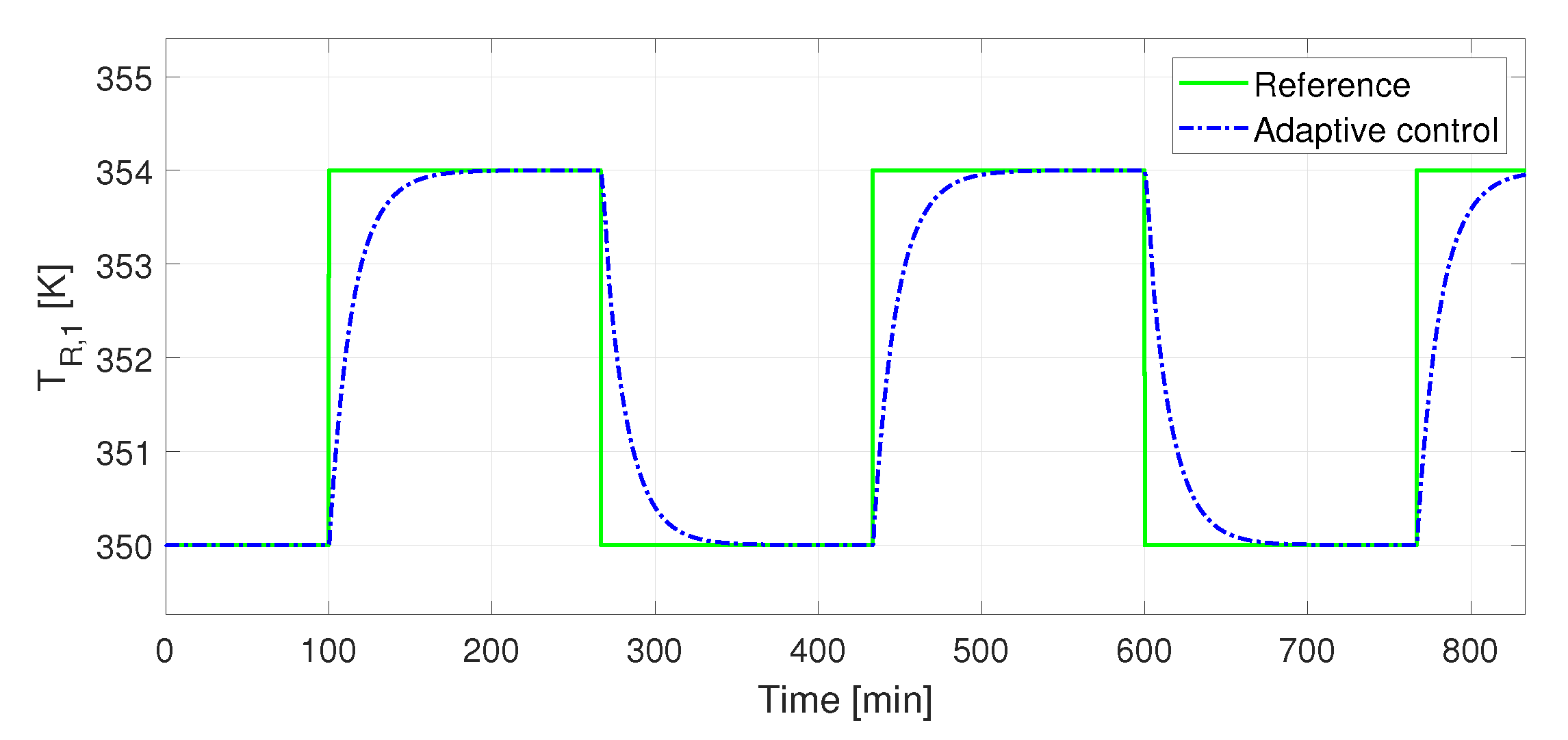
The first test scenario assesses the system response to sharp input disturbances. Thus, we simulated the closed-loop system with reference changes in $T_{R,1}$. The first shift started after $100\min$, then changes of $\pm 4\mathrm{K}$ were driven every $166\min$. The reference shift in $R_1$ alters the inlet condition of the subsequent reactor $R_2$, and the same is true for the set of second and third reactors.

For the adaptive control, we designed a polynomial $T_1\left(z^{-1}\right)$ to deal with reference tracking in the first reactor. We calculated it from $T_1\left(z^{-1}\right)=P_1\left(1\right)/B_1\left(1\right)$. In Figure 8, the reactor temperature $T_{R,1}$ is traced. The graph tracks the reference changes over time. One can observe that the reactor temperature stabilizes nearly 50 min after any change.

Temperature change in the reactors means an evolution of the concentration variables. The deviations in the input and output of $R_1$ cause indeed a fluctuation of the output concentration in $R_2$ and $R_3$. Figure 9 shows the concentration dynamics in the three reactors. On the other hand, it is worthy to note that the outlet temperature in reactors two and three are held close to the reference, which means that they, at all times, hold an isothermal operation. See in Figure 10 the temperature evolution.

The effort to manipulate the input variable to match the reference was more significant in the first reactor than it was for the downstream units. If the temperature in $R_1$ drops from a high temperature to the nominal value ($350\mathrm{K}$), the cold fluid flow steps up. In any case, in the driven test, the flow stayed within the allowable limits, which the valve features enforce (see Figure 11). For the driven tests, the control input in reactors $R_2$ and $R_3$ does not go beyond the operating limits. However, significant flow changes took place when the reference moved $\pm 4\mathrm{K}$. Given that $R_1$ operates at a higher temperature than the coming up units, the cooling jackets of reactors $R_2$ and $R_3$ carried lower down cold fluid flow (see Figure 11b,c, respectively).

The MPC control was unable to make the baseline change in the first reactor. Being a multivariable controller, added to the interaction between variables due to being a multivariable serial process, it was a difficult task to continue with the calculation of the control signals of the reactors $R_2$ and $R_3$ in such a way that a slow response was obtained, making it difficult to maintain the temperature. In reactors 2 and 3, the jacket flows $F_{J,2}$ and $F_{J,3}$ show a trend toward the maximum flow limit allowed by design and operation as shown in Figure 11b,c, respectively.

During the first 100 min of simulation, the behavior is similar to that with the adaptive control; however, after the disturbance is applied, the control effort makes a very abrupt change, from a value very close to the stable state up to the maximum flow allowed in the cooling jacket. Even so, this change is not enough to make the temperature change to the new reference. The control effort reaches the physical limits established in the design. The jacket flow signal of the first reactor saturates at the limit value of the restrictions, as can be seen in Figure 11a.

Figure 12a updates the parameters estimated in the course of the trajectory tracking in $R_1$. Likewise, Figure 12b,c update control parameters in reactors $R_2$ and $R_3$. Opposite to the $R_1$ update, the parameters estimates for reactors $R_2$ and $R_3$ fit at all times their optimal values, which correspond to the nominal point. In fact, the impact on the subsequent reactors, produced by the reference change in $R_1$, is weakened by the control loop of the first reactor.

5.2. Variations in the Auxiliary Services: Simultaneous Disturbances in $F_{J,1}$ and $T_{R_{in},1}$

Industrial plants operate, aided by services that supply heat or material streams to their units. These streams have disturbed variables that influence the processing units by random or periodic fluctuations. In the system of three reactors in series, disturbances can be sensed in the inlet temperature $T_{R_{in},i}$ of the reactors and the flow rate of their cooling jacket, $F_{J,i}$. The second test scenario evaluates the performance of the adaptive control scheme for damping input disturbances. To this end, we simulated the closed-loop system subject to simultaneous disturbances. The simulations were run with perturbations on the two input variables in $R_1$: $T_{R_{in},1}$ and $F_{J,1}$.

Now, the control objective is to reject simultaneous disturbances. We assumed that additive perturbations merge variations of the jacket flow of reactor $R_1$ and the reactor inlet temperature to simulate the system. Likewise, we suppose that the cooling fluid comes from an auxiliary service or another processing unit. Hence, the variations of the jacket flow were built as additive disturbances in the control signal, $F_{J,1}$. The input signals are periodical sinusoidal functions, applied at simulation time from $16\min$ to $810\min$. These evolved in time with distinct amplitudes and biases. The input signal is composed of a first sinusoidal wave with an amplitude of $\pm 15\%$ of the nominal $F_{J,1}$ and a frequency of $0.000955\mathrm{Hz}$, plus a bias, occurring until time $200\mathrm{s}$. The next $200\mathrm{s}$, the signal shifts to a sinusoidal wave with an amplitude of $\pm 10\%$ of the nominal $F_{J,1}$ and a frequency of $0.000795\mathrm{Hz}$. This wave train repeats itself to time $810\min$. 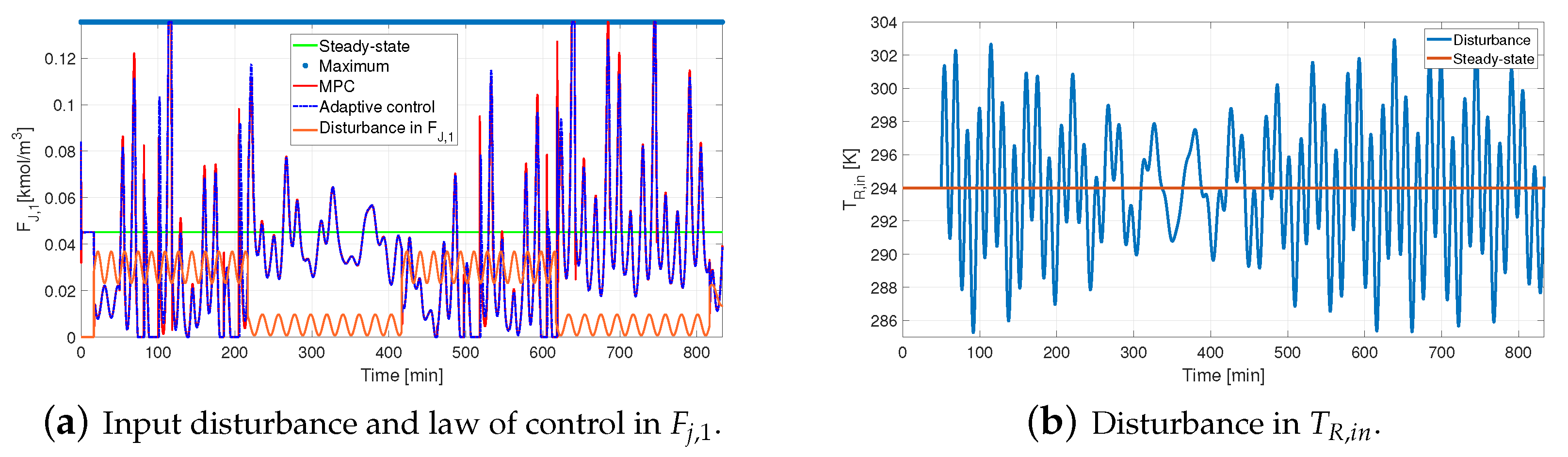In Figure 13a, the disturbance signal of the jacket flow is shown in orange.

Additionally, we ran the simulation test with disturbances in the reactor inlet temperature $T_{R_{in},1}$. Such changes in the inlet stream reproduce the impact of environmental shifts and interactions with other processes and auxiliary service equipment. The inlet temperature changed at $t=50\min$. This continuous disturbance signal was the sum of three sinusoidal functions with distinct amplitudes and frequencies (see Figure 13b). Three frequencies were chosen, $f_1=0.002\mathrm{Hz}$, $f_2=0.00698\mathrm{Hz}$, and $f_3=0.00681\mathrm{Hz}$. Their amplitude was $9\mathrm{K}$ around the nominal value.

The concurrent perturbations cause deviations of $\pm 0.6\mathrm{K}$ in the controlled variable in the first reactor (see Figure 14). The temperature of reactors $R_2$ and $R_3$ are close to their reference values. The disturbance in $R_1$ is damped, and its repercussion on the other reactors drops due to the control action in $R_1$. Figure 15 shows the concentration dynamics in the three reactors.

We handle performance indexes in

Table 2. Performance indicator of controllers simultaneous disturbance.

Performance Indicators
REACTOR	Controller	ISE	IAE × ${\mathbf{10}}^{\mathbf{3}}$	ITSE	ITAE × ${\mathbf{10}}^{\mathbf{5}}$
1	Adaptable	7.5	2.01	$2.25\times {10}^7$	1002
	MPC	351.8	1.02	$1.76\times {10}^7$	509
2	Adaptable	$6.1\times {10}^{-6}$	0.82	18.25	0.408
	MPC	0.0038	5.51	188.3	2.75
3	Adaptable	0.00013	9.52	390.04	4.76
	MPC	0.0031	10.14	157.02	5.07

to make a quantifiable test of the control performance. The ISE index helps to rate the efficacy of the adaptive control to hold on to the output variable near the reference. The substantial ITAE and ITSE point out that the signal oscillates. This result is not surprising, as the input disturbances are sinusoidal. Even if the controllers keep down their impact, slight oscillation stays over time.

Disturbance rejection is attained for both control laws in the first reactor $R_1$ with a similar control effort. See Figure 13a; in the first few minutes of the simulation, the controller counteracts the inlet temperature variation in the three reactors. On the other hand, the adaptive control does not lead to high flow feeding of the jacket. The highest effort also comes in the first few minutes of simulation for each reactor, as seen in Figure 16.

The control effort made by the MPC for the jacket flow of the third reactor has more aggressive changes and presents many oscillations during the entire simulation time compared to the jacket flow provided by the adaptive control (see Figure 16b). The expected behavior of the cooling flow of the third reactor must be “softer”, indicating the attenuation of the disturbances in the previous units.

The controller updated the parameters estimated after a disturbance in the jacket flow. The change of the parameters for reactor $R_1$ is shown Figure 17a. We also estimated online the parameters for reactors 2 and 3. Still, a minor divergence of their values was observed due to disturbance weakening by the control in the first reactor (see Figure 17b,c, respectively).

Some general remarks on the design and performance of the controller are as follows: Actuators in CSTR control loops are valves. A control valve is a device that manipulates a working fluid to compensate for disturbances and maintain the output at the set point. In this work, the control input is directly the cooling fluid flow, so we do not use a valve model to design the controller. This fact is equivalent to assuming that the valve instantaneously reaches a specific position or that the dead time and the time response are minor. We also consider that the control signal is not constrained, which means that the control design neglects the nonlinearities caused by input saturation.

For reactor tanks, the rule of thumb indicates that the flow fed through a valve can reach a value of two or up to three times the nominal value. Outside these limits, the control signal saturates, the closed-loop behavior degrades, and the system can become unstable. The designed control provides a conservative response with a smooth signal that does not exceed three times the nominal value. For this reason, the control law does not degrade. The temperature was subject to changes of up to $\pm 9\mathrm{K}$ around the nominal value for the simultaneous disturbance test. At the same time, the flow entering the jacket was perturbed with variations of up to $15\%$. Even with these significant disturbances, the control law did not exceed the possible physical limits.

Aspects of the control synthesis that aided in achieving the performance seen in the tests are as follows: the pole placement searched for a performance away from high frequencies but ensured closed-loop stability. The pole assignment gave robust stability, as the sensitivity functions fit perfectly within the robustness margins (Figure 7a). Disturbances at the inputs do not significantly influence the outputs, except in the third reactor when very low-frequency disturbances, such as a reference shift, are involved (Figure 7b). The control law provides high tolerance to disturbances at the control inputs since the input sensitivity curves are smooth curves with variations in a small range, and no rapid or large amplitude changes are shown over the entire frequency range (Figure 7c).

The control scheme has effectively regulated the concentration in the three reactors indirectly. In the first control test, the concentration oscillates (Figure 9). In any case, the conversion equals the reference or increases slightly, compared to the reference. The second test stabilizes the concentration at the reference with short pulses (Figure 15).

6. Conclusions

At the beginning of this paper, we gave an account of the most common types of disturbances in chemical plants. Inputs to such processes and disturbances were portrayed as signals within a short frequency span. Thus, we proposed an adaptive control scheme to reject narrow-bandwidth disturbances. Here, we describe the closed-loop system elements and the main outcomes.

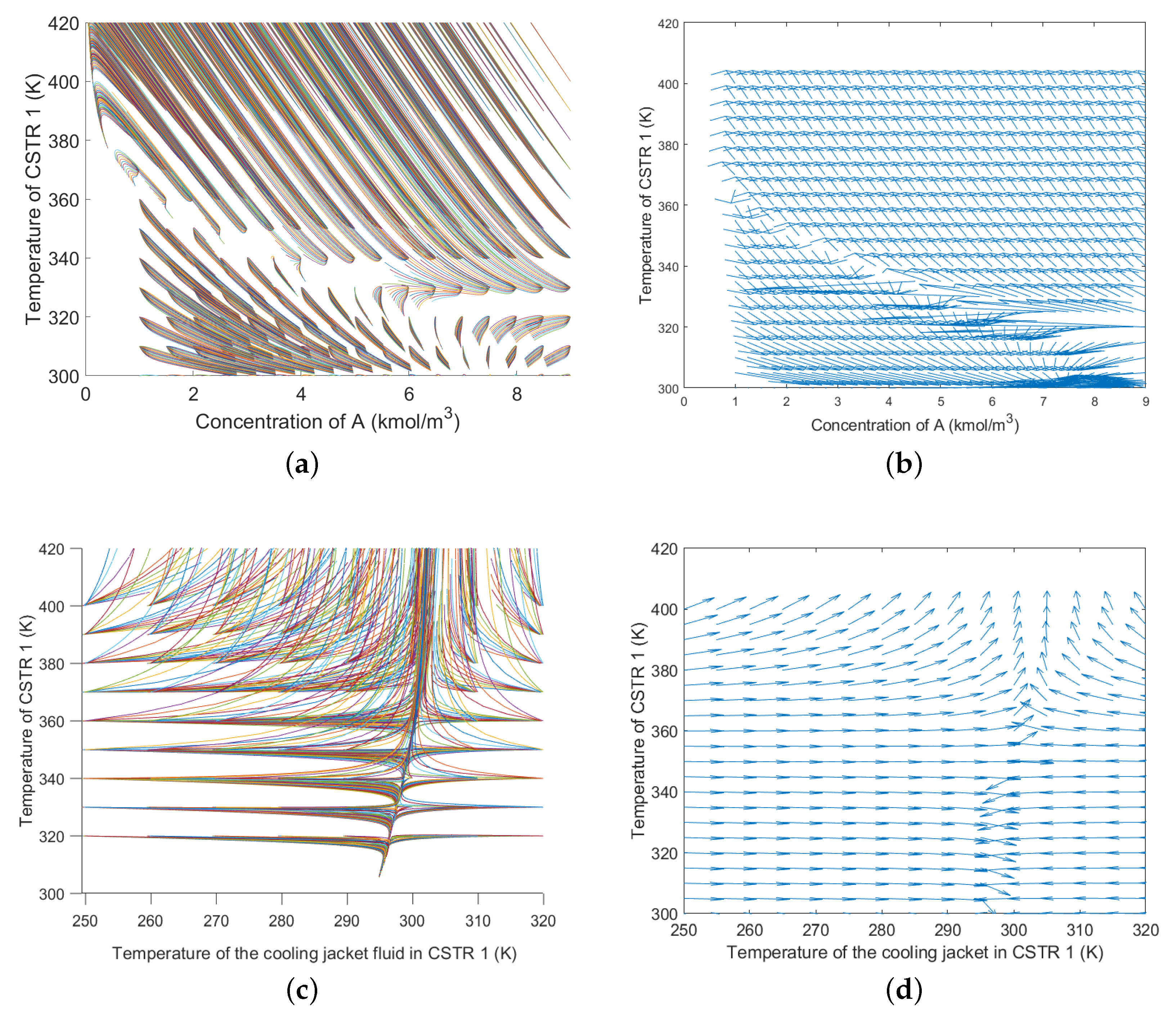
Reactors have been broadly used to investigate process control strategies because of their dynamic traits. We tested our control scheme in a 3-CSTR plant. This plant behavior is nonlinear and engages in interactions as the reactors are cascaded. The nonlinear mathematical model obeys the conservation equations and replicates these features. The reaction of A is exothermic and yields a product for which the concentration determines the product quality. The lower the concentration of A, the higher the reaction conversion. We studied the steady state behavior of $R1$ with the aid of phase portraits and the Van Heerden diagram. We concluded that $R1$ is liable to run in thermal instability regions, have multiple equilibrium points, and risk of thermal reactor runaway. Under these circumstances, temperature regulation is a better choice than direct concentration control. The first option leads to operating in safe regions and prevents the need for a state observer design to estimate a nonmeasurable variable. Because temperature strongly affects concentration, temperature control becomes an indirect composition control. The $R1$ unit effortlessly can lead to unsafe operation and low-quality products. It is indeed an intensified process that replaces a single reactor. The control in the serial process becomes more demanding than regulating a single reactor. However, the gain in safety, volume, efficiency, and cost show just cause for the control challenge.

The control scheme is composed of two parts. The first part is a fixed design, whereas the second engages an online update. The central control is an RS polynomial block structure. This compensator keeps the stability by pole placement based on a linearized model for the serial units given as a triangular matrix of transfer functions. The robust design concerned shaping the closed-loop sensitivity functions and checking the robustness margins, which engaged tolerance to non-linearities, unmodeled dynamics, output disturbances (sensor noise) and interaction between units in series. Then, a second part of the control scheme uses a recursive least square optimizing the filter Q to correct the disturbance model. Thus, adaptive control alludes to updating online the disturbance model rather than the control design. A filter estimated the input disturbance online. With this information, the closed-loop performance improved tolerance to input disturbances. An excitation injected through a Dirac delta function allowed abrupt disturbances to be modeled, then damped.

An S-type thermocouple was an element for temperature measurement in the plant simulator. This type of sensor has high accuracy and stability for applications with inert and oxidizing atmospheres. The closed-loop simulator included a dynamic thermal model of the sensor. On the other hand, the actuators were not modeled in the system. It is known that common undesired behaviors of control valves lead to closed-loop instability. Actuator saturation is one critical issue. However, our control design improved the pole placement by calibrating the sensitivity functions with compliance of robustness margins. This approach resulted in smooth control input, preventing input saturation issues for solid disturbances.

The control test consisted of two scenarios: the first one entered disturbances that mean sharp transients or reference changes. The second entered multiple input disturbances that stood for variations in the auxiliary services stream. The control goal was to hold the isothermal operation of the plant and, in an indirect form, the product concentration set point, despite the disturbances. The MPC is a well-established technique in advanced control for chemical processes. We confronted the adaptive controller effectiveness with that of an MPC. The trial of the two control schemes for the case of multiple input disturbances resulted in similar performance, but the MPC implies a more significant steady-state error. Otherwise, both control laws show low but persistent oscillations, but the control effort is more significant for the MPC, mainly in the second and third reactors. For the reference change scenario, we conclude that the effectiveness of the adaptive single input-single output control scheme surpassed that of the multivariable predictive controller, which demonstrates the control law tolerance to interactions of the multivariable plant. In brief, for the conducted tests, the controller parameters evolve significantly over time in both case studies. Thus, the tests confirmed the relevance of estimating and updating the model of unknown disturbances.