Article

Generalized Johnson Distributions and Risk Functionals

by
Christos Floros
1,
Konstantinos Gkillas
1 and
Christos Kountzakis
2,*
1
Department of Accounting and Finance, Hellenic Mediterranean University, 71004 Herakleion, Greece
2
Department of Statistics and Actuarial-Financial Mathematics, School of Sciences, University of the Aegean, Karlovassi, 83200 Samos, Greece
*
Author to whom correspondence should be addressed.
Mathematics 2022, 10(17), 3200; https://doi.org/10.3390/math10173200
Submission received: 20 July 2022 / Revised: 19 August 2022 / Accepted: 25 August 2022 / Published: 5 September 2022
(This article belongs to the Special Issue Advances in Financial Modeling)

Abstract

:
In this paper, we study the generalized Johnson distributions’ class and its applications in finance and risk theory. The recent literature on Johnson distributions displays a better gooodness of fitting for data coming from financial markets, such as portfolio returns. However, a gereral question in risk theory and finance is the following: Which class of distributions is more appropriate in order to determine the behaviour of data coming from financial markets and insurance claims? Another question is the following one: Is ther any class of distributions that is appropriate for calculations related to any kind of risk faced by financial isntitutions and insurance companies? The answer proposed to these questions is the use of generalized Johnson’s distributions. The parameters of such distributions are estimated by the order statistics of a single or more samples. Risk functionals represent a unified approach comprising every kind of risk metric. Risk functionals include value-at-risk and expected shortfall, coherent risk measures, and endpoints and thresholds. We deduce that the risk functionals sastisfy convexity—like properties with respect to finitely-mixed distributions. We also prove in detail that the empirical distribution is a reasonable way for the estimation of the above risk functionals. In the Appendix, we provide two numerical examples for fitting samples of portfolio returns under the Johnson’s transformation.

1. Introduction: Generalized Johnson Distributions and Their Use

In the present paper, we may consider ( Ω , F , P ) to be a non-atomic probability space. A random variable is some element of L 0 ( Ω , F , P ) , which is the vector space of F -measurable real-valued functions, being defined on Ω . The portfolio returns’ behavior is an initial motivation for the introduction of the class of generalized Johnson’s distributions. Such a motivation appears in the Appendix A. Specifically, the Johnson distribution with respect to the normal distribution may be used for this aim. As it is well-known, the Johnson transformation for Y with respect to the normal distribution W is as follows:
W : = Z μ σ = l o g ( Y ξ ξ + λ Y ) ,
where Z N ( μ , σ 2 ) and ξ , λ > 0 .
There are two seminal papers for the usual Johnson’s distributions, being [1,2]. The initial motivation for this section is that many data sets obtained from financial markets may be not well-fitted on some well-known distributions. Random variables that determine the behaviour of financial markets are usually called financial risk. variables. Under the Johnson transformation, these data-sets are well-fitted on a well-known distribution. In the Appendix A, we provide two examples of this. In [3], authors propose such a non-parametric approach. The goodness-of-fit testing we propose here is described below. We also prove that the generalized Johnson’s distributions and the maxima domains of attraction have the same tail behaviour. The maxima domains of attraction are usually used in order to estimate the ruin probability in life and non-life insurance. If WG, such that the moments E ( | W | ) , E ( W 2 ) are finite, then the distribution of Y is called the generalized Johnson’s distribution with respect to W. G is the cumulative distribution function of W. We may notice that the class of Cauchy distributions does not admit such a transformation since mean and variance are not well-defined in this case. Specifically, we have:
X : = W E ( W ) σ ( W ) = l o g ( Y ξ ξ + λ Y ) ,
where ξ , λ > 0 and σ ( W ) is the standard deviation of W. A random variable S : Ω R is a continuous random variable, if and only if the cardinal number of the values of X is equal to the cardinal number of R . The cumulative distribution function of Y is denoted by F Y . X corresponds to the normalization of W. W may not be normalized, and this is the case with the examples in the Appendix A at the end of the paper. Risk functionals include any real-valued function, whose domain is the cointinous distributions. For example, value at risk, expected shortfall, thresholds, and endpoints are examples of risk functionals. The endpoint and the threshold of a distribution are quite important in actuarial science because they estimate the size of a single large claim. The present paper may be compared to Ref. [4]. In the present paper, a specified distribution class is not considered. Ref. [4] also refers to the introduction of Johnson distributions, in order to achieve the “goodness-of-fit” for data coming from financial markets. The class of generalized Johnson distributions in the present paper is a non-parametric approach to this point. This is true since we require that first and second moments of G be finite. This assumption is required for the scope of “normalization” for G. A four-moments’ treatment estimation appears in [5,6] as well. In [7], the authors refer to the generalized Johnson distribution with respect to a normal distribution. Ref. [7] is important, since the authors apply the above distribution in credit risk modeling. Additionally, in [7] the assumption of the fact that both E ( | W | ) , E ( W 2 ) are not equal to infinity arises from the fact that W is normally distributed. This assumption is a little restrictive since in actuarial science and finance the distributions of claims and returns are not always normally distributed. Throughout the present paper, we assume that these moments are finite. Since in [7] is devoted to credit risk modeling, X may be a linear combination of other random variables, namely, X = i = 1 I a i C i , i = 1 , 2 , , I . C i may be either the variables used by credit rating institutions, or the more significant principal components arising form them. This approach is under examination due to the fact that some of these variables may be caterogical. Credit risk is actually the risk arising from the inablity of either a state or some other institution to pay the amount of money received by another financial institution. Finally, we have to mention that the seminal paper about coherent risk measures is [8]. In [9], the authors provide a complete review of every expected shortfall estimation method. A precise approach on estimating expected shortfall by using re-sampling methods arises in [10]. The convergence results arising in the present paper establish an estimation practice that is non-parametric, in the sense that is “distribution-free”. For a specified error bound ε > 0 , the size of the sample needed for the estimation of any risk functional is determined from the empirical cumulative distribution function. Risk management practice usually refers to a variety of risk ‘components’. The notion of risk functionals provides a unified approach of these risk components and their estimation by the notion of convergence as it arises in real analysis, together with the “convexity”-like properties, under finitely-mixed distributions. These properties are true for finitely-mixed generalized Johnson distributions since the corresponding random variables’ values are positive. Some recent literature related to thresholds and endpoints of finitely -mixed Lognormal Pereto distributions in [11,12,13]. Obviously, the risk functionals may be used in study of other sorts of risk, like liquidity risk and operational risk, which may included in the class of risk factors. The risk factors correspond to a ’holistic’ approach, including any kind of risk being faced by enterprises, banks, and insurance companny. The ’loading weights’ may be updated, relying, for example, on historical data. The distribution of such a risk factor corresponds to a time-dependent risk fuctional, which is under use for a specific kind of risk. This is the motivation for the use of finitely-mixed distributions and specifically for their risk functionals, while this expert systems’ aproach in risk management issues appears in [14,15,16]. The inequalities appearing in the last part of the section before the section related to the empirical distribution function show that, in any case, risk functionals mentioned here are very “close” to each other. Hence, for any risk factor, the same risk functional may be used for the quantification of it.

2. Parameter Estimation

As it is mentioned above, Y = ξ + ξ Q + λ Q Q + 1 = ξ + λ Q Q + 1 = ξ + λ R , where R = Q Q + 1 and Y is Q = e X and X = W E ( W ) σ ( W ) .
The parameters ξ and λ for a specific sample may be estimated by the order statistics of a sample. Let us consider a sample of m observations: ( Y 1 , Y 2 , , Y m ) and the corresponding ordered sample: ( Y ( 1 ) , Y ( 2 ) , , Y ( m ) ) . We also consider some ε , δ R , such that ξ 1 = Y ( m ) + ε > 0 and λ 1 = Y ( 1 ) + δ > 0 , such that
Y j ξ 1 > 0 ,
and
λ 1 + ξ 1 Y j > 0 ,
for any j = 1 , 2 , , m . Then, we may use the well-known Anderson–Darling test, see [17,18]. As we mentioned in the introduction, generalized Johnson distributions may be used in order to achieve a better “goodness-of-fit” for data coming from financial markets. We show it by a numerical example described at the Appendix A. After the references, we included the corresponding tables. For the data processing, we used the Minitab Software. In these examples, we suppose that ξ , λ take specific values. For this reason, we may call the Johnson transformation any transformation of the form Y = ξ + λ R , where ξ , λ are non-negative real numbers and λ > 0 . R = Q Q + 1 and Y is Q = e X , X = W E ( W ) σ ( W ) , while the cumulative distribution fuction of W is G. The “goodness-of-fit” results are quite similar both in the cases of ξ = 0 and ξ > 0 . In the first example of the Appendix A  ξ = 0 , while in the second one ξ = 1 . In both of the examples, we pose λ = 1 .

3. Thresholds and Endpoints

Definition 1.
A risk functional is any f : D R , where D is the set of cumulative distribution functions of continuous random variables.
Definition 2.
x F : = inf { x R | F ( x ) < 1 } .
If this infimum is a real number, then it is called F-threshold.
Lemma 1.
For any continuous random variable whose support is a subset of positive real numbers, x F is a real numeber.
Proof. 
If the support of F is a subset of the positive real numbers, then { x R + | F ( x ) < 1 } is a lower bounded subset of the real numbers. This set is non-empty. This is true since if we suppose that for any x R + F ( x ) 1 , this implies that for any x R + , F ( x ) = 1 . If this is true, P ( X x ) = 1 , for any x R + . This is true if X takes negative values, which is a contradiction.  □
Corollary 1.
For any Y, whose distribution is some generalized Johnson’s Distribution, x F Y is well-defined.
Proof. 
Let us suppose that for any ϵ > 0 , then F ¯ Y ( ϵ ) = 0 . This is a contradiction because it implies that P ( Y 0 ) = 1 , namely, that P ( ξ + ξ Q + λ Q Q + 1 0 ) = 1 . □
Definition 3.
x E , F : = inf { x R | F ( x ) = 1 } .
If this infimum is real number, it is called F-endpoint.
The above definition of the F-endpoint appears in [19].
If the significance level a is equal to 1, we notice that x E , F = V a R 1 ( F ) , according to the above definition.
Both thresholds and endpoints are risk functionals, and they are related to value at risk and expected shortfall. We recall the definition of value at risk V a R a , under a significance level a ( 0 , 1 ) :
V a R a ( X ) = inf { t R | F X ( t ) a } ,
or more exactly
V a R a ( F X ) = inf { t R | F X ( t ) a } .
Expected shortfall E S a under a significance level a ( 0 , 1 ) is a risk functional since any random variable X L 0 ( Ω , F , P ) corresponnds to the cumulative distribution function F X of X. Hence, E S a ( X ) = E S a ( F X ) .
Definition 4.
A finitely-mixed distribution is a distribution whose cumulative distribution function is F ( x ) = i = 1 k q i F i ( x ) , where q i > 0 and i = 1 k q i = 1 .
Theorem 1.
If the support of F i is a subset of the positive real numbers for any i = 1 , 2 , , k ,, then x F = i = 1 k q i x F i .
Proof. 
Since if x F i 0 for any i = 1 , 2 , , k ,
x F = inf { x R + | F ( x ) < 1 } =
inf { x R + | i = 1 k q i F i ( x ) < 1 } =
= inf { ( i = 1 k q i ) x R + | i = 1 k q i F i ( x ) < 1 } =
= i = 1 k q i inf { x R + | F i ( x ) < 1 } =
= i = 1 k q i x F i .
 □
The above result refers to the threshold of finitely mixed distributions. We deduce the equivalent result for the endpoint of finitely-mixed distributions:
Theorem 2.
If the support of F i is a subset of the positive real numbers for any i = 1 , 2 , , k , then x E , F = i = 1 k q i x E , F i .
Proof. 
Since if x E , F i 0 for any i = 1 , 2 , , k ,
x E , F = sup { x R + | F ( x ) = 1 } =
= sup { x R + | i = 1 k q i F i ( x ) = 1 } =
= sup { ( i = 1 k q i ) x R + | i = 1 k q i F i ( x ) = 1 } =
= i = 1 k q i sup { x R + | F i ( x ) = 1 } =
= i = 1 k q i x E , F i .
 □
Theorem 3.
If the support of F i is a subset of the positive real numbers for any i = 1 , 2 , , k , then V a R a ( F ) = i = 1 k q i V a R a ( F i ) for any a ( 0 , 1 ) .
Proof. 
Since if V a R a ( F i ) 0 for any i = 1 , 2 , , k ,
V a R a ( F ) = inf { x R + | F ( x ) a } =
inf { x R + | i = 1 k q i F i ( x ) a } =
= inf { ( i = 1 k q i ) x R + | i = 1 k q i F i ( x ) i = 1 k q i a } =
= i = 1 k q i inf { x R + | F i ( x ) a } =
= i = 1 k q i V a R a ( F i ) .
 □
Theorem 4.
If the support of F i is a subset of the positive real numbers for any i = 1 , 2 , , k and F i are cumulative distribution functions of random variables lying in L 1 ( Ω , F , P ) , then E S a ( F ) = i = 1 k q i E S a ( F i ) for any a ( 0 , 1 ) .
Proof. 
From the above theorem, by using the relation E S a ( F i ) = 1 a 0 a V a R u ( F i ) d u , for any i = 1 , , k .  □
The above results are also valid if F i , i = 1 , , k are cumulative distribution functions of generalized Johnson distributions since they actually take positive values.
Theorem 5.
If the support of F is a subset of the positive real numbers, then x F V a R a ( F ) , for any a ( 0 , 1 ) .
Proof. 
The conclusion is a consequence of the properties of real numbers. { t R + | F ( t ) a } is a subset of { t R + | F ( t ) < 1 } , for any a ( 0 , 1 ) .  □
Theorem 6.
If the support of F is a subset of the positive real numbers and F is the cumulative distribution functions of a random variables lying in L 1 ( Ω , F , P ) , then
E S a ( F ) x F ,
for any a ( 0 , 1 ) .
Proof. 
The conclusion is a consequence of the equality E S a ( F ) = 1 a 0 a V a R u ( F ) d u .  □
We may also appent to seminal literature about law-invariance of expected shortfall. Such a reference is [20]. Another risk functional related to Orlicz spaces is the entropic value at risk, which is established in [21].
Risk functionals are kinds of so-called risk factors. A linear combination of risk functionals j = 1 d a j f j , d N , a j R + , j = 1 , , d and f j , j = = 1 , , d is a risk functional defined on the same probability space mentioned initially. This probability measure is related to the information obtained by anyone of these risk factors. As we may notice, the set A + B = { c R + | c = a + b , a A , b B } if A , B are non-empty subsets of positive real numbers, while t A = { c R + | a A } if t is also a positive real number.

4. Approximation of Risk Functionals

In the previous section, we discussed the notion of risk functionals. A question regarding risk functionals is how we may estimate them, using a specific sample. We remind the defintition and the properties of empirical cumulative distribution. If we consider a sample from the distribution of some continuous random variable X, which is denoted by ( X 1 , X 2 , , X n ) , the empirical distribution of it is defined as follows:
F ^ n ( t ) = 1 n i = 1 n 1 { X n t } .
The indicator function of the event A is denoted by 1 A . The Glivenko–Cantelli theorem is the following result, concerning an empirical distribution function:
lim n F ^ n ( t ) F ( t ) = 0 .
Hence, the Glivenko–Cantelli theorem meaning is that the empirical distribution function F ^ n converges to the (cumulative) distribution function of the random variable X, under the supremum norm. Hence, the above convergence is uniform, hence it is also point-wise. The Glivenko–Cantelli theorem may be used for the approximation of both F-threshold and F-endpoint. The Glivenko–Cantelli theorem is also true, if F is replaced by the tail function F ¯ = 1 F . The empirical distribution function is replaced by the empirical tail function F ^ ¯ n = 1 F ^ n . The natural number n N in the next definitions, and the results denote the size of the sample, being used for the calculation of the empirical distribution’s values. The Glivenko–Cantelli theorem is seminally established in [22,23]. There exist two papers appeared under the same title and they were published in the same Journal in 1933. The one was written by V. Glivenko and the other one was written by F.P. Cantelli.
Definition 5.
x E , F ^ n = inf { t R | F ^ n ( t ) = 1 } is the F-empirical endpoint for any n N .
Definition 6.
V a R a ( F ^ n ) = inf { t R | F ^ n ( t ) a } is the F-empirical value-at-risk, for any a ( 0 , 1 ) and any n N .
Definition 7.
E S a ( F ^ n ) = 1 a 0 a V a R u ( F ^ n ) d u is the F-empirical expected shortfall, for any a ( 0 , 1 ) and any n N .
From the Glivenko–Cantelli theorem, we obtain the validity of the following propositions:
Proposition 1.
x E , F ^ n x E , F .
Proof. 
The uniform convergence of the empirical distribution function implies the point-wise convergence of it to the cumulative distribution function F. Moreover, x E , F ^ n are real numbers for any n N .  □
Proposition 2.
For any a ( 0 , 1 ) , V a R a ( F ^ n ) V a R a ( F ) .
Proof. 
The uniform convergence of the empirical distribution function implies the point-wise convergence of it to the cumulative distribution function F. V a R a ( F ^ n ) are real numbers for any n N .  □
Proposition 3.
For any a ( 0 , 1 ) , E S a ( F ^ n ) E S a ( F ) .
Proof. 
For the proof of the above proposition, we use the dominated convergence theorem, with respect to the Lebesgue measure on the closed interval [ 0 , 1 ] of the real numbers.  □
Definition 8.
A risk measure ρ : L 1 ( Ω , F , P ) R , is law-invariant if X = d Y , implies ρ ( X ) = ρ ( Y ) . X = d Y means that F X = F Y almost everywhere, with respect to the Lebesgue measure on R .
Remark 1.
A law-invariant risk measure is a risk functional, under the definition given in the previous sections.
Proposition 4.
For any law-invariant, coherent risk measure ρ : L 1 ( Ω , F , P ) R , ρ ( F ^ X n ) ρ ( F X ) , for any X L 1 ( Ω , F , P ) . F ^ X n is the empirical distribution function of X, as it is defined above.
Proof. 
From the above proposition and [10], where any law-invariant coherent risk measure ρ : L 1 ( Ω , F , P ) R is a convex combination of expected shortfall risk measures. Hence, the sequence of real numbers ( ρ ( F ^ X n ) , n N ) is well-defined in this case. If r i > 0 and E S a i are such that ρ = i = 1 k r i E S a i , where i = 1 k r i = 1 and a i ( 0 , 1 ) for any i = 1 , , k . Then, ρ ( X ) = ρ ( F X ) for any X L 1 ( Ω , F , P ) . ρ ( F ^ X n ) = i = 1 k r i E S a i ( F ^ X n , where F = F X for any n N .  □
Corollary 2.
For any law invariant coherent risk measure ρ : L 1 ( Ω , F , P ) R and any X L 1 ( Ω , F , P ) , then ρ ( F ^ X n ) ρ ( F X ) .
Proof. 
From the previous proposition and the propoerties of convergent real-valued sequences.  □
The above results imply the ‘intuition’ that both value-at-risk and the expected shortfall of the empirical distribution approximate both value-at-risk and expected shortfall for the distribution of any continuous random variable. We notice that such considerations hold for a random variable whose distribution is actually a generalized Johnson distribution, especially if this lies in L 1 ( Ω , F , P ) .

5. Recommendations and Conclusions

Coming back to both of the initial questions. The first one is Which class of distributions is more appropriate in order to determine the behaviour of data coming from financial markets and insurance claims. The second question is if there any class of distributions that is appropriate for calculations related to any kind of risk faced by financial isntitutions and insurance companies. We proposed that the class of Generalized Johnson Distributions is the appropriate class for both of the above questions. We also propose the notion of risk functional as a unified approach on law-invariant risk metrics. The main question for further study is how to modify an algorithmic approach for the calculations’ part. Namely, how is it possible for the risk management part of either a bank or an insurance company to accept or to reject an internal model and coonsequently the whole of quantification of a risk factor. Such an approach, where internal risk management, external risk management, and enterprise risk management are the main risk factors for an enterprise having a positive effect on any performance index of it, specifically appears in [15]. We point out that to measure these factors’ values, the specific risk functionals may be changed or may lead to a certain type of value similar to value-at-risk for some distribution of them. This separation comprises three subsignificant factors: internal models are related to forecasting the default risk, and external risk factors refer to the situation of the economy as a whole. By the word ‘economy’, we may understand either a branch of enterprise or a national economy lending money to these enterprises. Enterprise risk management may be understood as a situation of improving the balance sheet/accounting variables of an enterprise. Generalized Johnson distribution may be useful for the quantification of these risk factors.

Author Contributions

All authors have equally contributed in the published version of the manuscript’s formulation. All authors have read and agreed to the published version of the manuscript.

Funding

This research received no external funding.

Data Availability Statement

The datasets generated during and/or analyzed during the current study are available from the corresponding author on reasonable request.

Conflicts of Interest

There is not any conflict of interest concerning this paper.

Appendix A

We present two examples for goodness-of-fit, in order to deduce that generalized Johnson distributions are appropriate for this purpose. We obtained a portfolio of stocks comming from the Athens’ Stock Exchange, consisting of the “closing-of-the-date-value” per share for the stock of National Bank of Greece and the National Electricity Company of Greece. The data refer to dates between 31 March 2020 and 20 January 2021. As a return-per-date, we consider the portfolio value V ( t + 1 ) V ( t ) . Since the portfolio weights are θ 1 = 2 3 and θ 2 = 1 3 , the daily value of the portfolio is equal to
V ( t ) = θ 1 S 1 ( t ) + θ 2 S 2 ( t ) ,
where S 1 ( t ) is the closing-per-date value for one shere of the stock of National Bank of Greece and S 2 ( t ) is the closing-per-date for one share of the stock of the National Electricity Company of Greece. We tested the goodness-of-fit for the returns on the Exponential Distribution. The goodness-of-fit test being used is the Anderson–Darling test. Both the value of it and the corresponding probability plot appear after the References. We may observe that the exponential distribution is not well-fitted on it. Note that the Johnson transformation Y = Q Q + 1 , where Q = e X and X corresponds to the random variable of the returns X, which corresponds to the sample V ( t + 1 ) V ( t ) , for any t = 1 , , 200 . We apply the Anderson–Darling test on the data of coming from Y. As it appears from the corresponding value of the test and the probability plot, the greatest part of the sample is well-fitted to the normal distribution. The normal distribution arises as a consequence of the goodness-of-fit testing. We also note that both distributions are non-heavy-tailed, and the support of the exponential distibrution is unbounded. The graphs for the goodness-of-fit are at the end of the manuscript. We have to mention that Minitab Software was used for this data processing.
Another example is the following one, whose corresponding probability plots and Anderson–Darling test values appear at the last pages of the paper: we notice that the Johnson transformation Y = 1 + Q Q + 1 , where Q = e X and X corresponds to the random variable of the returns X, which corresponds to the sample V ( t + 1 ) V ( t ) , for any t = 1 , , 300 . We notice that Y is one among the random variables arising from the corresponding Johnson transformation. The portfolio of stocks comming from the Athens’ Stock Exchange consisted of the “closing-of-the-date-value” per share for the stock of Lamda Real Estate and the National Betting Company of Greece (OPAP). The data refer to dates between 8 August 2017 and 18 October 2018. As a return-per-date, we consider the portfolio value V ( t + 1 ) V ( t ) . Since the portfolio weights are θ 1 = 1 4 and θ 2 = 3 4 , the daily value of the portfolio is equal to
V ( t ) = θ 1 S 1 ( t ) + θ 2 S 2 ( t ) ,
as well. As it is noticed through the corresponding probability plots and the associated values of the Anderson–Darling test:
1.
The sample of the returns’ variable X is ’marginally’ well-fitted on any normal distribution.
2.
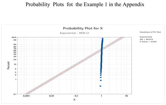
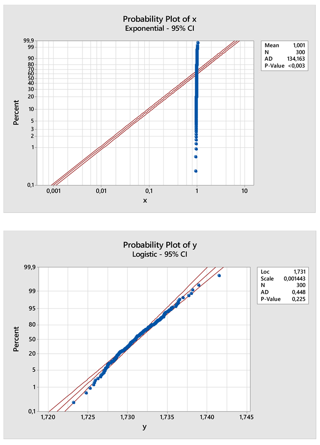
The sample of the returns’ variable X is out-of-fit, with respect to the exponential distribution.
3.
The sample of the Johnson transformation Y = 1 + Q Q + 1 , where Q = e X is well-fitted on the logistic distribution. X is the random variable of the sample above, namely, the sample of the returns’ variable.
Mathematics 10 03200 i001
Mathematics 10 03200 i002
Mathematics 10 03200 i003

References

  1. Johnson, N.L. Systems of Frequency Curves Generated by Methods of Translation. Biometrika 1949, 36, 149–176. [Google Scholar] [CrossRef] [PubMed]
  2. Johnson, N.L. Bivariate Distributions Based on Simple Translation Systems. Biometrika 1949, 36, 297–304. [Google Scholar] [CrossRef] [PubMed]
  3. Corlu, C.G.; Corlu, A. Modelling exchange rate returns: Which flexible distribution to use? Quant. Financ. 2015, 15, 1851–1864. [Google Scholar] [CrossRef]
  4. Simonato, J.G. The Performance of Johnson distributions for Computing value at risk and expected shortfall. J. Deriv. 2011, 19, 7–24. [Google Scholar] [CrossRef]
  5. Lien, D.; Stroud, C.; Ye, K. Comparing VaR Approximation Methods that Use the First Four Moments as Inputs. Commun. Stat. Simul. Comput. 2016, 45, 491–503. [Google Scholar] [CrossRef]
  6. Tuenter, H.J.H. An algorithm to determine the parameters of SU-curves in the johnson system of probabillity distributions by moment matching. J. Stat. Comput. Simul. 2001, 70, 325–347. [Google Scholar] [CrossRef]
  7. Huang, Z.; Kwok, Y.K. Efficient risk measures calculations for generalized CreditRisk+ models. Int. J. Theor. Appl. Financ. 2021, 24, 2150012. [Google Scholar] [CrossRef]
  8. Artzner, P.; Delbean, F.; Eber, J.M.; Heath, D. Coherent Measures of Risk. Math. Financ. 1999, 9, 203–228. [Google Scholar] [CrossRef]
  9. Nadarajah, S.; Zhang, B.; Chan, S. Estimation methods for expected shortfall. Quant. Financ. 2014, 14, 271–291. [Google Scholar] [CrossRef]
  10. Inui, M.L.; Kijima, M. On the significance of expected shortfall as a coherent risk measure. J. Bank. Financ. 2005, 29, 853–864. [Google Scholar] [CrossRef]
  11. Cooray, K.; Ananda, M.M.A. Modeling actuarial data with a composite LognormalPareto model. Scand. Actuar. J. 2005, 5, 321334. [Google Scholar]
  12. Pigeon, M.; Denuit, M. Composite Lognormal–Pareto model with random threshold. Scand. Actuar. J. 2011, 3, 177–192. [Google Scholar] [CrossRef]
  13. Scollnik, D.P.M. On composite Lognormal-Pareto models. Scand. Actuar. J. 2007, 1, 20–33. [Google Scholar] [CrossRef]
  14. Akatov, N.; Mingaleva, Z.; Klaĉková, I.; Galieva, G.; Shaidurova, N. Expert Technology for Risk Management in the Implementation of QRM in a High-Tech Industrial Enterprise. Manag. Syst. Prod. Eng. 2019, 27, 250–254. [Google Scholar] [CrossRef]
  15. Hanggraeni, D.; Ślusarczyk, B.; Sulung, L.A.K.; Subroto, A. The impact of internal, external and enterprise risk management on the performance of micro, small and medium enterprises. Sustainability 2019, 11, 2172. [Google Scholar] [CrossRef]
  16. Mingaleva, Z.; Akatov, N.; Butakova, M.; Akatov, N.; Butakova, M. A syndinic approach to enterprise risk management. In Lecture Notes in Networks and Systems; LNNS; Springer: Cham, Switzerland, 2022; Volume 315, pp. 293–305. [Google Scholar]
  17. Anderson, T.W.; Darling, D.A. Asymptotic theory of certain “goodness-of-fit” criteria based on stochastic processes. Ann. Math. Stat. 1952, 23, 193–212. [Google Scholar] [CrossRef]
  18. Anderson, T.W.; Darling, D.A. A Test of Goodness-of-Fit. J. Am. Stat. Assoc. 1954, 49, 765–769. [Google Scholar] [CrossRef]
  19. Resnick, S.I. Tail Equivalence and Its Applications. J. Appl. Probab. 1971, 8, 136–156. [Google Scholar] [CrossRef]
  20. Acerbi, C.; Tasche, D. On the coherence of expected shortfall. J. Bank. Financ. 2002, 26, 1487–1503. [Google Scholar] [CrossRef]
  21. Ahmadi- Javid, A. Entropic Value-at-Risk: A New Coherent Risk Measure. J. Optim. Theory Appl. 2012, 155, 1105–1123. [Google Scholar] [CrossRef]
  22. Cantelli, F.P. Sulla determinazione empirica delle leggi di probabilitá. Giorn. Ist. Ital. Attuari 1933, 4, 421–424. [Google Scholar]
  23. Glivenko, V. Sulla determinazione empirica delle leggi di probabilitá. Giorn. Ist. Ital. Attuari 1933, 4, 92–99. [Google Scholar]
Publisher’s Note: MDPI stays neutral with regard to jurisdictional claims in published maps and institutional affiliations.

