Abstract
This paper extends the conditional autoregressive range (CARR) model to the multivariate CARR (MCARR) model and further to the two-stage MCARR-return model to model and forecast volatilities, correlations and returns of multiple financial assets. The first stage model fits the scaled realised Parkinson volatility measures using individual series and their pairwise sums of indices to the MCARR model to obtain the fitted volatilities. Then covariances are calculated to construct the fitted variance–covariance matrix of returns which are imputed into the stage-two return model to capture the heteroskedasticity of assets’ returns. We investigate different choices of mean functions to describe the volatility dynamics. Empirical applications are based on the Standard and Poor 500, Dow Jones Industrial Average and Dow Jones United States Financial Service Indices. Results show that the stage-one MCARR models using asymmetric mean functions give better in-sample model fits than those based on symmetric mean functions. They also provide better out-of-sample volatility forecasts than those using CARR models based on two robust loss functions. We also find that the stage-two return models with constant means and multivariate Student-t errors give better in-sample fits than the Baba–Engle–Kraft–Kroner generalised autoregressive conditional heteroskedasticity models. The estimates and forecasts of value-at-risk (VaR) and conditional VaR based on the best MCARR-return models for each asset are provided and tested using backtests to confirm the accuracy of the VaR forecasts.
Keywords:
range-based volatility; correlation; multivariate CARR-return model; value-at-risk; conditional value-at-risk MSC:
37M10; 62H99; 62M10
1. Introduction
Financial markets can be very volatile, meaning that asset prices can change a lot in a given period. Volatility is a statistical measure of the dispersion of returns for an asset within a short time period. Market volatility is mainly reflected in the deviation of asset future value expectations. It can present significant investment risk or opportunities for astute investors. Many investors trade in portfolios which made up of individual position, each with its own volatility profile. These individual variations, when combined, create a measure of portfolio risk or volatility which can be very different from the risk or volatility of individual position, depending on how they correlate with each other. Hence, investors should align their portfolios not only with relevant expected returns but also with manageable risk level which is subject to the risk profile of the portfolio constituents.
Understanding individual risk dynamics and their cross-dependency can shed light on future returns and volatilities of the portfolio constituents and guide portfolio strategies. Besides, forecasting assets’ future returns and volatilities is also a key factor when pricing options contracts. As volatility is time-varying and unobservable, it needs to be estimated. Researchers estimate volatility mainly in two ways: fitting time series return models and measuring volatility directly using daily or intraday prices.
To model the volatility dynamics, the last few decades have seen the popularisation of many return models based on daily closing prices and their extensions to incorporate volatility measures. Generalised autoregressive conditional heteroskedasticity (GARCH) models are constructed using daily closing prices, discarding all intraday price movements and estimating volatility as a latent process in the return series [1]. The volatility dynamic for the variance is expressed as a deterministic function of the lagged squared innovations and its lagged variances. An extension of the deterministic volatility in GARCH model to stochastic volatility is the stochastic volatility (SV) model introduced by [2]. Since then, GARCH and SV become two main classes of models that describe the time-varying autocorrelated volatility process.
Instead of treating volatility as a latent process, some researchers endeavoured to measure volatility directly. Refs. [3,4,5,6] proposed different types of range-based volatility measures based on the opening, highest, lowest and closing prices. With the availability of high frequency asset price data, another approach to improve the accuracy of daily volatility measure is the realised volatility measures making use of intraday price information. Extensions of realised variance [7] to many more realised volatility measures have been introduced to improve the efficiency of the daily volatility measures [8,9]. However, these volatility measures, like returns, have random noise. Hence, they are often fitted to some models to smooth out the noise and/or provide additional source of information. In realised GARCH model [10], they are incorporated into the volatility equation via a term from a separated realised volatility model.
Alternatively, volatility models have been proposed and applied directly to the volatility measures. These models should capture features in volatility clustering, such as long-term persistence, short-term persistence and leverage effect. Ref. [11] proposed the conditional autoregressive range (CARR) model to model the volatility measures directly. Compared to the GARCH model, these volatility models model the volatility measures, not returns, as a stochastic instead of deterministic process. They can be further extended to provide volatility estimates in the return models to capture the volatility clustering in the returns. This results in the two-stage volatility and return models that fit the CARR models in the first stage and impute the fitted volatilities into the returns models to capture the heteroskedasticity of returns in the second stage [12,13]. These two-stage CARR-return models are different from the GARCH and SV models that use only the information of returns. Instead, the two-stage models use both return and volatility information and model them as two stochastic processes. Hence, the two-stage models also differ from the realised GARCH model since the latent volatility equation is omitted although the realised GARCH model also has two stochastic processes for returns and realised volatilities.
Although the univariate GARCH models are popular in financial econometrics, they neglect the contemporaneous dependency over a set of assets, stock market indices or exchange rates. These contemporaneous dependency induces return and volatility spillover between multiple assets and are important in many financial applications such as portfolio optimisation and hedging strategy formulation. Without capturing the contemporaneous dependency through covariance measures, the univariate GARCH models are limited in assessing the risk of a portfolio. Multivariate modelling and forecasting of asset returns can capture the dynamics of the covariance matrix and, hence, have prominent applications in portfolio optimisation. The increasing interaction and interconnection between financial markets have motivated the need for reliable modelling and forecasting of the contemporaneous dependencies of financial asset returns. However, the variance–covariance matrix of asset returns is not directly observable in practice. Traditional volatility models treat it either as deterministic latent quantities such as the multivariate GARCH (MGARCH) models or as stochastic latent quantities such as the multivariate SV (MSV) models [14]. These models estimate the latent variance–covariance matrix using returns.
Extending from the univariate setting, the variance–covariance matrices are, in general, modelled as a linear function of lagged observed and modelled variance–covariance matrices, multiplied to some coefficient matrices to be estimated. However, as the number of assets increase, the number of parameters in a multivariate model may explode causing problems of model and, hence, parameter instabilities. This problem is called the curse of dimensionality. Moreover, the variance–covariance matrices in the MGARCH models should be positive definite [15]. The vectorisation GARCH (VEC-GARCH) model introduced by [16] suffers from the high dimensionality and non-positive definiteness problems. Since then, various MGARCH models were developed to address the dimensionality and positive definiteness issues. The Baba–Engle–Kraft–Kroner GARCH (BEKK-GARCH) model proposed by [17] adopts quadratic long and short-term persistent matrices to ensure positive-definiteness and reduce the number of parameters. Moreover, the dynamic conditional correlation (DCC)-GARCH model [18] offers direct modelling of variances and correlation and is very appealing. Multivariate extension also applies to the SV model family. Ref. [19] proposed the MSV model, which allows the variances and covariances to evolve through time. In the model, a set of asset returns is driven by some latent factors which are specified as SV processes. The dimension of the parameter space of this model is manageable as it only increases linearly with the number of assets being modelled. Hence, the MSV model has fewer parameters than the MGARCH model.
In recent years, different range-based MGARCH models have been proposed to improve the modelling efficiency. They use different ways to incorporate the range information. Among them, [20] proposed to calculate covariance using the variance of each component and their pairwise sum so that range-based volatility measures such as Parkinson high-low [3] can be applied. Then the range-based variance–covariance matrix can be constructed. The BEKK-High-Low-GARCH model proposed by [21] adopted this range-based variance–covariance matrix as the short-term persistence matrix, replacing the product of return residual vector in the standard BEKK-GARCH model.
A similar idea applies to the DCC-GARCH model for the short-term persistence matrix in the correlation matrix equation. Ref. [22] proposed the co-range DCC-GARCH model which adopts the range-based correlation matrix standardised from the range-based variance–covariance matrix which replaces the product of standardised return residual vector in the standard DCC-GARCH model. For the univariate model, Ref. [23] proposed range-GARCH (RGARCH) model in which the squared return residual in the volatility equation is replaced by the Parkinson [3] volatility measure. Then, Ref. [24] proposed the DCC-RGARCH model which estimates the short-term persistence matrix using the product of standardised return residual vector from the RGARCH model. Another approach uses the range information to standardise return residuals. Ref. [25] estimates the short-term persistence matrix using product of return residual vector standardised by dividing each component from the mean of the univariate CARR model for that component. These models incorporate a range-based volatility measure in different ways to improve estimates of covariance or correlation matrix for returns and increase the accuracy of covariance, variance and correlation forecasts compared to MGARCH models that use only closing prices.
On the other hand, extensions of CARR models for volatility measures to multivariate settings imply the modelling of some positive definite variance–covariance matrix measures using some distributions defined for matrices. These highly sophisticated matrix distributions include the Wishart [26] and matrix-F [27] distributions. Alternatively, ref. [20] extended the CARR model to the multivariate CARR (MCARR) model to model the variances of individual asset return and their pairwise sum. Through the estimated variance of pairwise sum, the estimated covariance of the asset pair can be determined, and so, the estimated variance–covariance matrix can be similarly constructed. An obvious advantage of the MCARR model is that the modelling of covariance via the variance of pairwise sum allows the same CARR model structure to be applied. Otherwise, one needs to adopt some covariance models with a different distribution assumption for a different support. However, Ref. [20] did not provide a numerical demonstration for the application of the proposed model.
Similar to the two-stage CARR-return models of [13] the MCARR model can also be extended to a two-stage MCARR-return model. However, empirical studies using the MCARR and two-stage MCARR-return models are lacking in the literature. This paper aims to provide a practical framework for the application of these models. Our approach is similar to [21] in modelling covariance rather than correlation matrix. However, we apply the stochastic MCARR model to the vector of range-based variance of each component and their pairwise sum instead of taking the range-based variance–covariance matrix as the short-term persistence matrix in the deterministic covariance model for the GARCH model. Our approach is more interpretable and direct. To estimate the parameters of these models, we consider four popular methods, namely, the maximum likelihood (ML) [28,29], quasi ML [11,30,31], Bayesian [12,32,33] and estimating functions [34]. We choose the ML method since the likelihood function can be completely specified under the MCARR and two-stage MCARR-return models and the models can be easily implemented using the MATLAB optimisation package fmincon.
To select some best performing models, the forecast performance for volatilities can be evaluated by some loss functions. Apart from the root mean squared forecast error and the mean absolute forecast error, [35] proposed a loss function family that can be adopted to assess model predictability for both in-sample estimates and out-of-sample forecasts. The scalar parameter in the loss function family enables the loss function to cover a wide variety of shape, ranging from symmetric loss to asymmetric loss, with heavier penalty either on under-prediction or over-prediction. Ref. [35] claimed that these loss functions are robust to the choice of volatility proxy. Then the best performing two-stage MCARR-return model can be applied to provide forecast risk measures such as value-at-risk (VaR) [36] and conditional VaR (CVaR) [37], which are essential tools to measure the potential loss of an asset. The performance of VaR for returns can be assessed using some backtests based on counts of tail losses that exceed VaR [38,39].
The contribution of this paper is threefold. Firstly, we propose the MCARR model to study the dynamics of volatility and correlation of assets’ returns. We adopt asymmetric mean functions in the MCARR model to capture the leverage effects. We fit the efficient scaled realised Parkinson volatility measure of each index series and their pairwise sums of indices to the MCARR model to obtain in-sample estimates and forecasts of volatilities. The covariances and, hence, correlations of pairwise indices are calculated using the fitted volatilities of individual and pairwise sums of indices. We also investigate the performance of MCARR model with asymmetric and symmetric mean functions. The accuracy of volatility forecasts relative to the volatility proxy based on a scaled realised volatility measure is compared using two robust loss functions proposed in [35]. Secondly, we show how the volatility and covariance estimates from the MCARR models are imputed into the return models to model the variance–covariance matrix of returns in the two-stage MCARR-return model. The modelling performance of the two-stage MCARR-return model is compared with BEKK-GARCH models. Lastly, we provide forecasts of various VaR and CVaR for returns and tail quantile (TQ) and tail conditional expectation (TCE) for closing prices based on the best fitted two-stage MCARR-return models. The accuracy of these VaR forecasts is further tested using the Kupiec unconditional coverage (KUC) [38] and Christoffersen independent (CI) [39] tests.
The remainder of this paper is organised as follows. Section 2 introduces volatility measures that are used in this study. Section 3 describes MCARR and the two-stage MCARR-return models with different mean functions. Section 4 provides empirical applications to some daily index series. Performance of in-sample estimation and out-of-sample forecast of volatilities and returns are evaluated and compared with univariate CARR model and BEKK-GARCH models. The best model for each pair of indices is used to provide one-day-ahead forecasts of VaR and CVaR for returns and TQ and TCE for closing prices. Finally, Section 5 concludes the paper.
2. Realised Volatility Measures
Let be the price of an asset at day t. It follows the geometric Brownian motion
where is a drift for , is a volatility parameter and is the standard Brownian motion. The logarithmic price then satisfies
by Ito’s lemma. The logarithmic price process follows a Brownian motion with drift parameter and volatility parameter . Although (1) and (2) are defined on continuous time, they are often discretised in real applications as most asset price series are measured over discrete time points. The logarithmic return (hereafter referred to as return) of an asset price is given by
where denotes the logarithmic closing price at day t. It is also called close-to-close (CC) return. Returns can also be measured intraday (called open-to-close (CO)) as
where denotes the logarithmic opening price at day t. Compared with CC return , research shows that intraday CO return contributes more to total return. Intraday return is of particular importance for day traders, who use daytime gyrations in stocks and markets to make trading profits. Hence, we adopt intraday CO return . For volatility, the stationary process in (2) is often extended to be a time-varied process to capture the volatility clustering in returns. Ref. [3] proposed an unbiased measure for such volatility process, called Parkinson (PK) measure, which is given by
where and denote the highest and lowest logarithmic prices of day t, respectively. Using more intraday information, [9] proposed the scaled realised PK (SRPK) measure given by
where is the PK measure of day , is the realised PK (RPK) measure of day t which is given by
where and are the highest and lowest logarithmic prices in the l-th () interval of day t, and trading days (3 months) is the optimal scaling period suggested by [40]. This SRPK measure using more intraday information is more efficient and the scaling factor which is the multiple before in (4) adjusts for the downward bias due to infrequent trading. To assess the performance of SRPK measure in the empirical study, we use the scaled realised CO (SRCO) measure as a proxy to the true volatility . The SRCO measure is given by
by applying the idea of scaled realised measures to realised CO (RCO) measure defined as
is the intraday volatility measure of day and trading days (3 months) is the optimal scaling period suggested by [40].
To measure covariances, these range-based measures fail. Ref. [7] introduced the realised sample covariance between return series i and j as
where and are respectively the last and first trading logarithmic prices in the l-th () interval of day t. This realised sample covariance measure is defined in a similar way as the realised sample variance measure using high frequency data and can be used to estimate the off-diagonal entries in the variance–covariance matrix of asset returns. However, models for the covariance measures are different from models for variance measures because covariances have a real support whereas variances are always positive. To avoid modelling variance and covariance using different model structures, [20] proposed the MCARR model by using only variance measures and estimating the covariance using the variance of the pairwise sum as detailed in the next section.
3. Multivariate Volatility and Return Models
We describe the proposed two-stage MCARR-return models and compare the models with BEKK-GARCH models.
3.1. Two-Stage MCARR-Return Model
3.1.1. Stage-One MCARR Model
Suppose there are K asset returns . Let denote a K-dimensional column vector of K asset returns at day t. Their volatilities are estimated by the SRPK measures, that is,
using (4). Ref. [20] proposed the MCARR model by using only variance measures and estimating the covariance between return series and using
The new series is the sum of the returns for assets i and j at day t. The advantage of MCARR model is that it by-passes the modelling of covariance with a real support so that the same CARR model defined on can be applied to model all , and where indicates which variance that corresponds to the sum of returns of the pair. The SRPK volatility measures of the pairwise sums are given by
for and . Hence, the total number of variances to be modelled becomes . For example, when , and , that is, the third volatility measure corresponds to the sum of returns for the (2,1) pair. The and as required in in (5) and then in (4) are obtained by summing the corresponding highest and the lowest logarithmic prices of two assets, that is,
according to [41]. As l increases,
as desired. The first stage MCARR model for the SRPK volatility measure () is given by
where , is the dimensional vector of conditional expectations at day t given the information set up to day , and is the vector of errors. Equivalently, (14) can be written as
The errors are assumed to follow a multivariate log-normal (MLN) distribution, that is,
where is a dimensional vector of location of parameters. The probability density function (pdf) of is given by
We standardise the MLN distribution such that E, then the vector in (17) is eliminated by replacing for .
The mean function in (14) can be modelled by p ordered autoregressive terms, q ordered persistence terms and the presence (denoted by MCARR(p,q,1)) or absence (denoted by MCARR(p,q,0)) of leverage effect. In general, the mean function is given by:
where the coefficient vector measures the inherent uncertainty in the range-based volatility measure, the coefficient matrices and measure the short-term (autoregressive) and long-term (persistence) impacts of shocks to the range-based measure, respectively, is a scalar of one () or zero (), and the coefficient matrices in and measure the leverage effect. MCARR model is a multivariate extension of the univariate CARR model given by
where and e the scalar parameters. CARR model with and leverage effect () is denoted by CARR(1,1,1). Similarly, MCARR model with a symmetric mean function (absence of leverage effect, ) and is denoted by MCARR(1,1,0). Then (18) can be written as
where and are the parameters to be estimated for . To reduce the number of parameters, we assume symmetric autoregressive and persistence effects, that is, and for . Then (20) can be written as
Since parameter and indicate the short term and long term volatility spillover on asset j by the volatility of asset i, the symmetric persistence effect assumption, that is, and imply that the volatility spillover on asset i by the volatility of asset j is the same as the volatility spillover on asset j by the volatility of asset i.
To account for the asymmetric impact of returns on the next day conditional variance, we extend the mean function in (18) to the asymmetric mean function (when ) which is given by
where is a vector of returns of day with for . When , this model is called MCARR(1,1,1) model with leverage effect. To reduce the number of parameters, we further assume and , that is, the cross leverage effect is zero. Then (22) is given by
Similarly, we consider and for . When and, hence, , (23) is given by
The number of parameters in these mean functions is when and, hence, . It becomes 15 when dropping the leverage effect. The number of model parameters will be 6 more after counting in (16), that is, 27 and 21 respectively for the models with and without leverage effect. We also remark that parameters and indicate the short term and long term volatility spillover on asset 1 by the volatility of asset 2.
To derive the ML estimator, the log-likelihood (LL) function is given by
where is the conditional pdf of and is the vector of parameters. The conditional pdf of is obtained from in (17) after we consider standardisation with E and transformation according to (14). The LL function is given by
where . The ML estimator of is evaluated by
where represents the vector space of all parameters and can be obtained using a suitable optimisation package such as in MATLAB.
To attain the best model fit, we select models with the largest LL value and/or the smallest Akaike information criterion (AIC) given by
where is the number of parameters in the model. While LL provides guidance of the best model fit, AIC penalises complicated model with a penalty proportional to the number of parameters.
3.1.2. Stage-Two Multivariate Return Model
At the second stage, we impute the fitted values as volatility estimates in the multivariate return model. Let be a vector of returns of K assets at day t. To model , we consider return model
where is the time-varying conditional expectation at day t given the information set up to day , is a diagonal matrix of scaling factors , and are assumed to follow a multivariate Student-t (MVT) distribution with mean , scale matrix and degrees of freedom, that is, MVT with the pdf
The LL function of is given by
where is the conditional pdf of and is the vector of parameters. The conditional pdf is obtained from in (29) using transformation according to (28). The LL function is given by
The mean vector adopt a constant mean and an autoregressive of order 1 (denoted by AR(1)) mean structure, that is, , where is a dimensional coefficient matrix, or
and
Equation (28) could be written as
The scale matrix is estimated by
where are given in (21) and (24) for the first K components of MCARR(1,1,0) and MCARR(1,1,1) models, respectively, , for , is a mapping from the entry in to the entry in , and according to (10) where . For example, when so that , and where in (21) and (24) for MCARR(1,1,0) and MCARR(1,1,1) models, respectively. The vector of model parameters for the return model is . If the AR(1) term is dropped, .
3.2. BEKK-GARCH Model
We compare the performance of the two-stage MCARR-return models with BEKK-GARCH models. The asset returns follow a MGARCH process if the innovations has the representation
where is a square matrix such that and is an unobservable independent and identically distributed random error vector with . It follows that is measurable with respect to information generated up to day , denoted by . The BEKK-GARCH() specification of [17] developed a general quadratic form for the conditional scale matrix to estimate the volatilities and returns. The volatility model is given by
where is a lower triangular matrix and and are matrices. When and , the model in (35) contains parameters to be estimated and implies the following dynamic models for the elements of :
where and and the baseline coefficient matrix is assumed to be symmetric. When the coefficient matrices and are further simplified to diagonal, the number of parameters becomes 7. The scaled errors in (34) may follow multivariate normal (MVN) or MVT distributions with identity scaled matrix for the full BEKK-GARCH() (FBEKK-GARCH()) and diagonal BEKK-GARCH() (DBEKK-GARCH()) models in the empirical study.
4. Application
4.1. Data and Volatility Measures
We consider Standard and Poor’s (S&P) 500 index (), Dow Jones Industrial Average (DJIA) index (), and Dow Jones United States Financial Services Index (DJUSFI) (). These data have a sampling frequency of 1-minute and cover from 1 May 2013 to 31 May 2019 for a total of 1527 trading days. We select these three return series because they represent large and liquid markets in the United States. Hence, the data reflect market conditions in the same region, and there is no concern about the non-synchronous data collection. The return series of S&P 500 is highly correlated with DJIA () but less correlated with DJUSFI () while the correlation between DJIA and DJUSFI returns is relatively lower (). In the preliminary study, we first calculate the PK and RPK measures defined in (3) and (5) respectively for these indices and rescale them up by multiplying . We further calculate the SRPK measure defined in (4) based on these two measures. We analyse the volatility measures of the three returns series, namely, SRPK, SRPK and SRPK in (9), and their pairwise sum series, namely, SRPK, SRPK and SRPK in (11).
The summary statistics for these six volatility measures are reported in Table 1. All six measures have a high level of positive skewness and kurtosis. The large values of the Ljung–Box (LB) test statistic for all these measures provide evidence of significant autocorrelation up to 12 lags. Figure 1 displays the histogram, autocorrelation function (ACF) and time series plots of SRPK measures for these six volatility series. The histograms display heavy skewness whereas the ACFs demonstrate high autocorrelation. These high autocorrelations justify the use of MCARR model with long-term persistence. The results also agree with the large skewness and LB test statistics in Table 1. The time series plots in Figure 1 display considerable volatility clustering for all series and they are particularly volatile during the period of July to December 2015. This period covers the sharp drop in stock prices in August 2015 due to fears from the potential breakup of contagion of Eurozone because of Greece’s financial woes, the China’s slowing growth, the oil’s steep slide and the dollar’s strength. There are also concerns about the effect of the Federal Reserve’s first interest rate hike in seven years since 2008. This severe volatility of stock market indices continues until the end of the year and can be seen from the time series plots in Figure 1.

Table 1.
Summary statistics of SRPK measures from 1 May 2013 to 31 May 2019 for S&P 500, DJIA, DJUSFI and their pairwise combined indices.
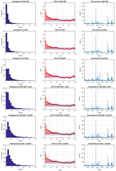
Figure 1.
Histogram, ACF and time series plots for SRPK measures from 1 May 2013 to 31 May 2019 with S&P 500, DJIA, DJUSFI and their pairwise sum indices.
4.2. Volatility Modelling and Forecast
The MCARR models can be applied to assess the pairwise dependency between the three asset returns through the modelling of variances and covariances over time. Models are implemented using fmincon in MATLAB. Since MCARR models contain many parameters, the search for starting values in running fmincon is more demanding. In general, we set parameter estimates from the univariate CARR model for each return series as the starting values and set the cross component parameters such as in (21) and in (16) to be very small. In the first stage, we model the SRPK measures using MCARR models and consider two different mean functions, denoted by MCARR(1,1,0) and MCARR(1,1,1) models, respectively. When modelling each volatility measure, the errors are assumed to follow a MLN distribution defined in (17). All models have only first order terms () to reduce the complexity of the model. The parameter estimates defined in (17), (21) and (24), the LL and AIC of each model are displayed in Table 2. The results show that the parameter estimates are mostly positive and significant. The significance of and in (21) and (24), respectively, confirms the short term and long term volatility spillover effects. The fitted volatilities of the six models in Table 2 are used to estimate in the return model for the two-stage MCARR-return model according to (33). In general, MCARR(1,1,1) model with 27 parameters outperforms MCARR(1,1,0) model with 21 parameters due to larger LL and smaller AIC values.
Table 2.
Parameter estimates, standard errors (in parentheses), model performance measures LL and AIC for in-sample estimation of the MCARR(1,1,0) and MCARR(1,1,1) models with the pairwise combined indices. Models with boldface LL and AIC are the best models.
Figure 2 displays the in-sample fits in the variance and correlation plots using MCARR(1,1,0) and MCARR(1,1,1) models. The correlation plots in the grey background are obtained from MCARR(1,1,1) model while the remaining correlation plots are obtained from MCARR(1,1,0) model. Both models are able to capture the volatilities and correlation of returns for each data pair. The fitted correlation plots of the pairwise return series show high level of correlation with averages of 0.9418, 0.8660, 0.8478 for MCARR(1,1,0) model, and 0.9412, 0.8663, 0.8478 for MCARR(1,1,1) model which agree with the average observed correlation coefficient of 0.9604, 0.8953, 0.8795, respectively.
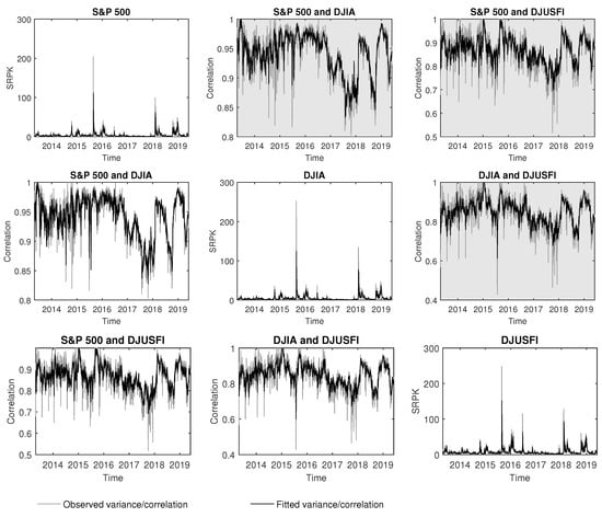
Figure 2.
Plots of in-sample fits of variance and correlation using MCARR(1,1,0) and MCARR(1,1,1) (in grey background) models with S&P 500, DJIA and DJUSFI indices.
We also compare the performance of the MCARR model with the univariate CARR models in (19), denoted by CARR(1,1,0) (symmetric mean function) and CARR(1,1,1) (asymmetric mean function), respectively, with log-normal error distribution. We perform one-day-ahead forecast from 3 June 2019 to 30 August 2019 giving a total of 64 daily variance forecasts. We assess the predictive performance of these variance estimates and forecasts by comparing them to the respective volatility proxy using SRCO measure in (6) based on the robust loss (RL) function given by
where is the forecast volatility, is the estimated volatility proxy using SRCO measure, is a scalar parameter which indicates different robust and homogeneous loss functions. The degree of homogeneity is equal to . Ref. [35] claimed that these loss functions are robust to the choice of volatility proxy and covers a wide variety of shapes, ranging from symmetric loss (; mean squared error) to asymmetric loss, with heavier penalty either on under-prediction () or over-prediction (). Moreover, the choice of corresponds to the popular quasi-likelihood (QLIKE) loss. If the loss due to under-prediction is more expensive, one may choose to set a heavier penalty for under-prediction with . We consider RL function with and . Table 3 shows that the variance estimates using CARR(1,1,1) model outperforms those using CARR(1,1,0), MCARR(1,1,0) and MCARR(1,1,1) models giving the lowest average loss with both and for the in-sample fit of all indices. This is suitable when the loss due to under-prediction is more expensive. For the out-of-sample forecasts, MCARR(1,1,1) model for S&P 500 and DJIA outperforms the rest of the models for both levels. For DJUSFI, forecasts using CARR(1,1,0) model achieve the smallest average loss when whereas forecasts using MCARR(1,1,1) model achieves the smallest average loss when . These variance estimates and forecasts for each index and pairwise sum from the MCARR model are imputed into the stage-two return models as described in the next section.
4.3. Return Model and Forecast
The summary statistics of daily returns for S&P 500, DJIA and DJUSFI indices are reported in Table 4. As kurtosis for all of the three indices are greater than three, the distributions of these indices have kurtosis higher than normal. Figure 3 graphs the histogram, ACF and time series plots for daily returns of S&P 500, DJIA and DJUSFI indices. The histograms display approximately symmetric and leptokurtic distributions and the ACF plots show weak persistence. The time series plots exhibit volatility clustering. These clustered returns give rise to higher peaks in the histograms. These peaks are much higher than the peak of normal density in red line confirming the higher than normal kurtosis for the return distributions. Hence, the results justify the use of MVT distribution with a constant mean or AR(1) mean structures to capture the high kurtosis and weak autocorrelation.
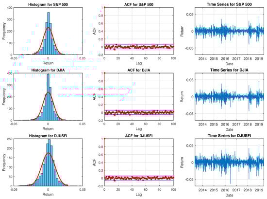
Figure 3.
Histogram, ACF and time series plots for daily returns of S&P 500, DJIA and DJUSFI indices from 1 May 2013 to 31 May 2019.
The second stage return model in (32) is fitted to the three asset returns and is estimated using the fitted from MCARR(1,1,0) and MCARR(1,1,1) models applied to SRPK volatility measures as in (21) and (24). As the results show that the AR(1) terms of stage-two return models are not significant, we provide the results of the return model with a constant mean in Table 5. Parameter estimates, LL and AIC are displayed in Table 5. The results show significance of all parameters at 5% level. The scaling parameters which adjust to be the unbiased estimator of are closed to one indicating the unbiasedness of the volatility measures for . Moreover, DJUSFI index seems to provide a higher level of returns among the other two indices (in agreement with sample mean) with larger mean estimates as indicated in Table 5. The degrees of freedom () for the MVT distribution are estimated to be around 5 to 6, indicating high kurtosis and confirming with the numerical measures and plots. Finally, models with the largest LL and the smallest AIC for each index pair as highlighted in Table 5 are selected for the return and price forecasts.
Table 3.
Robust loss functions at two asymmetric levels (b = ) for in-sample estimates and out-of-sample volatility forecasts using CARR (univariate) and MCARR (multivariate) models fitted to SRPK measures for S&P 500, DJIA and DJUSFI indices and compared to SRCO measure as the volatility proxy. The best model with the lowest average RL in each row is highlighted in boldface.
| Index | RL | CARR | MCARR | |||||||
|---|---|---|---|---|---|---|---|---|---|---|
| (1,1,0) | (1,1,1) | (1,1,0) | (1,1,1) | (1,1,0) | (1,1,1) | (1,1,0) | (1,1,1) | |||
| In-sample | S&P 500 | () | 8.0113 | 7.6172 | 8.3019 | 8.1238 | 8.0758 | 8.0154 | - | - |
| () | () | 0.2122 | 0.2036 | 0.2403 | 0.2253 | 0.2163 | 0.2137 | - | - | |
| DJIA | () | 10.556 | 10.127 | 10.780 | 10.590 | - | - | 10.605 | 10.553 | |
| () | () | 0.2201 | 0.2133 | 0.2499 | 0.2330 | - | - | 0.2241 | 0.2227 | |
| DJUSFI | () | 12.863 | 12.361 | - | - | 12.647 | 12.535 | 12.706 | 12.588 | |
| () | () | 0.1968 | 0.1907 | - | - | 0.1949 | 0.1936 | 0.1961 | 0.1945 | |
| Out-of-sample | S&P 500 | () | 1.8689 | 1.8207 | 1.9699 | 0.3699 | 1.8334 | 1.8173 | - | - |
| () | () | 0.2000 | 0.2115 | 0.2098 | 0.0601 | 0.2000 | 0.2019 | - | - | |
| DJIA | () | 1.6859 | 1.6237 | 1.7854 | 0.3438 | - | - | 1.6442 | 1.6724 | |
| () | () | 0.1662 | 0.1648 | 0.1665 | 0.0484 | - | - | 0.1648 | 0.1657 | |
| DJUSFI | () | 2.1305 | 4.4748 | - | - | 2.2588 | 2.2254 | 2.2560 | 2.2540 | |
| () | () | 0.1162 | 0.2199 | - | - | 0.1164 | 0.1157 | 0.1193 | 0.1178 | |
Remark: The subscripts ij in MCARR(1,1,0)ij and MCARR(1,1,1)ij for some i < j and i, j = 1, 2, 3 refer to i and j data pair.
Table 4.
Summary statistics of daily returns from 1 May 2013 to 31 May 2019 for S&P 500, DJIA and DJUSFI indices.
Table 4.
Summary statistics of daily returns from 1 May 2013 to 31 May 2019 for S&P 500, DJIA and DJUSFI indices.
| Summary Statistics | S&P 500 | DJIA | DJUSFI |
|---|---|---|---|
| mean | 18.702 | 18.963 | 24.545 |
| median | 45.714 | 53.483 | 93.577 |
| variance | 529,219 | 567,147 | 930,425 |
| skewness | −0.4501 | −0.3887 | −0.5750 |
| kurtosis | 4.0672 | 4.0951 | 3.6553 |
| minimum | −3947.3 | −4273.7 | −6329.2 |
| maximum | 4332.8 | 4564.1 | 4773.2 |
| LB, Q | 4.2167 | 4.7614 | 4.2159 |
| LB, Q | 7.7828 | 7.0345 | 7.6066 |
† Measures of location and dispersion are rescaled by multiplying 105.
We compare the performance of in-sample model fit of returns using the two-stage MCARR-return models, MCARR(1,1,0) and MCARR(1,1,1), with the popular BEKK-GARCH models in (35) such as FBEKK-GARCH and DBEKK-GARCH in which the coefficient matrices and are full or diagonal, respectively. We assign errors in (34) to follow MVN or MVT distributions and apply MATLAB free codes called the MFE Toolbox of Professor Kevin Sheppard to conduct parameter estimations. The models have order where the subscripts represents the three series of S&P 500, DJIA and DJUSFI and with indicates the pair of return series; hence, the models are (1,1), (1,1) and (1,1). Parameter estimates, LL and AIC are displayed in Table 6. The results are compared with those from MCARR(1,1,0) and MCARR(1,1,1) models displayed in Table 5. In general, the results show that MCARR(1,1,0) and MCARR(1,1,1) models outperform BEKK-GARCH(1,1) models with larger LL and smaller AIC values for each pair of indices.
Table 5.
Parameter estimates, standard errors (in parentheses), model performance measures LL and AIC for in-sample estimation of the return model for the two-stage MCARR-return model using volatility estimated from MCARR(1,1,0) and MCARR(1,1,1) volatility models. Models with boldface LL and AIC are the best models used in forecasting.
| S&P 500 and DJIA | S&P 500 and DJUSFI | DJIA and DJUSFI | ||||
|---|---|---|---|---|---|---|
| Return | MCARR | MCARR | MCARR | |||
| Model | (1,1,0) | (1,1,1) | (1,1,0) | (1,1,1) | (1,1,0) | (1,1,1) |
| 0.3067 | 0.3022 | 0.2891 | 0.2817 | 0.3431 | 0.3504 | |
| (0.1170) | (0.1267) | (0.1281) | (0.1194) | (0.1287) | (0.1235) | |
| 0.3084 | 0.3167 | 0.3758 | 0.4055 | 0.4806 | 0.4912 | |
| (0.1196) | (0.1314) | (0.1892) | (0.1705) | (0.1804) | (0.1708) | |
| 0.9965 | 0.9921 | 0.9270 | 0.9423 | 0.9614 | 0.9604 | |
| (0.0168) | (0.0191) | (0.0184) | (0.0172) | (0.0176) | (0.0201) | |
| 1.0120 | 1.0012 | 0.9624 | 0.9667 | 0.9691 | 0.9669 | |
| (0.0189) | (0.0194) | (0.0238) | (0.0184) | (0.0193) | (0.0222) | |
| 5.6716 | 6.0415 | 5.3052 | 5.8563 | 6.4431 | 6.2247 | |
| (0.4133) | (0.6267) | (0.3357) | (0.4734) | (0.4716) | (0.6569) | |
| LL | 12,937 | 12,936 | 11834 | 11,853 | 11,733 | 11,728 |
| AIC | −25,863 | −25,862 | −23,658 | −23,695 | −23,456 | −23,445 |
† Estimates and standard errors are rescaled by multiplying 103.
4.4. VaR and CVaR Forecasts and Risk Forecast Performance Measures
The two-stage MCARR-return model can provide forecasts of VaR and CVaR risk measures. We evaluate these risk measures for the returns in (28) using one-day-ahead forecasts and univariate marginal distributions. Specifically, the lower sided VaR forecast for K asset returns are given by
where is a vector of one, , and is the inverse distribution function of a Student-t distribution with degrees of freedom. Each component of the lower VaR is the -percentile of the marginal distribution given by
Table 6.
Parameter estimates and model performance measures LL and AIC for in-sample estimation of the DBEKK-GARCH(1,1) and FBEKK-GARCH(1,1) models. Models with boldface LL and AIC are the best for each index pair.
Table 6.
Parameter estimates and model performance measures LL and AIC for in-sample estimation of the DBEKK-GARCH(1,1) and FBEKK-GARCH(1,1) models. Models with boldface LL and AIC are the best for each index pair.
| Error Distribution | MVN | MVT | ||||||||||
|---|---|---|---|---|---|---|---|---|---|---|---|---|
| Model Type | DBEKK-GARCH | FBEKK-GARCH | DBEKK-GARCH | FBEKK-GARCH | ||||||||
| (1,1) | (1,1) | (1,1) | (1,1) | (1,1) | (1,1) | (1,1) | (1,1) | (1,1) | (1,1) | (1,1) | (1,1) | |
| 0.1828 | 0.1692 | 0.1558 | 0.1701 | 0.1978 | 0.1938 | 0.1661 | 0.1215 | 0.1210 | 0.1649 | 0.1896 | 0.1877 | |
| 0.1722 | 0.2123 | 0.1981 | 0.1539 | 0.2401 | 0.2248 | 0.1556 | 0.1593 | 0.1493 | 0.1544 | 0.2343 | 0.2201 | |
| 0.0694 | 0.1290 | 0.1340 | 0.0680 | 0.1566 | 0.1707 | 0.0670 | 0.1117 | 0.1138 | 0.0671 | 0.1559 | 0.1644 | |
| 0.4623 | 0.3480 | 0.3456 | 0.4623 | 0.4554 | 0.4575 | 0.4605 | 0.3124 | 0.3210 | 0.4605 | 0.4540 | 0.4582 | |
| - | - | - | 0.0629 | 0.0029 | 0.0104 | - | - | - | 0.0220 | −0.0083 | −0.0230 | |
| - | - | - | 0.0683 | 0.3540 | 0.0229 | - | - | - | 0.0089 | 0.1370 | 0.3910 | |
| 0.4623 | 0.3200 | 0.3167 | 0.4623 | 0.4554 | 0.4575 | 0.4605 | 0.2980 | 0.2961 | 0.4605 | 0.4540 | 0.4582 | |
| 0.8607 | 0.9008 | 0.9084 | 0.8607 | 0.8505 | 0.8517 | 0.8606 | 0.9301 | 0.9289 | 0.8606 | 0.8514 | 0.8512 | |
| - | - | - | 0.1420 | 0.0620 | 0.0210 | - | - | - | 0.0357 | −0.0180 | −0.1300 | |
| - | - | - | 0.0899 | 0.4580 | 0.3120 | - | - | - | 0.0112 | 0.1810 | 0.5760 | |
| 0.8607 | 0.9071 | 0.9113 | 0.8607 | 0.8505 | 0.8517 | 0.8606 | 0.9291 | 0.9316 | 0.8606 | 0.8514 | 0.8512 | |
| - | - | - | - | - | - | 11.100 | 6.0926 | 6.1433 | 11.100 | 11.100 | 11.100 | |
| LL | 12,804 | 11,732 | 11,597 | 12,801 | 11,716 | 11,579 | 12,921 | 11,838 | 11,708 | 12,920 | 11,805 | 11,674 |
| AIC | −25,594 | −23,452 | −23,180 | −25,580 | −23,409 | −23,136 | −25,826 | −23,661 | −23,400 | −25,818 | −23,587 | −23,324 |
† Estimates are rescaled by multiplying 102. ⋆ Estimates are rescaled by multiplying 105.
For the upper sided VaR, . The lower and upper CVaR are the conditional expected value of below and above its VaR, respectively, and they are defined as
and
respectively, where is the univariate Student-t pdf of .
The VaR forecasts of returns calculated for five confidence levels, 99%, 95%, 90%, 80% and 50% based on the multivariate return model in (28) using the two-stage MCARR-return model and SRPK volatility measures are presented in the two left panels of Figure 4. The plots in the grey background indicate the results obtained from the return model for the two-stage MCARR-return model by imputing the volatility estimates from the MCARR(1,1,1) model, whereas the rest are by imputing the volatility estimates from the MCARR(1,1,0) model. Then the asset price forecasts are transformed from the VaR return forecasts called TQ which is defined as
where . If VaR in (42) is replaced with CVaR, TCE is obtained. Figure 4 also displays the observed and fitted closing price forecasts and their 95% confidence limits of TQ and TCE for the asset closing price forecasts in the two right panels.
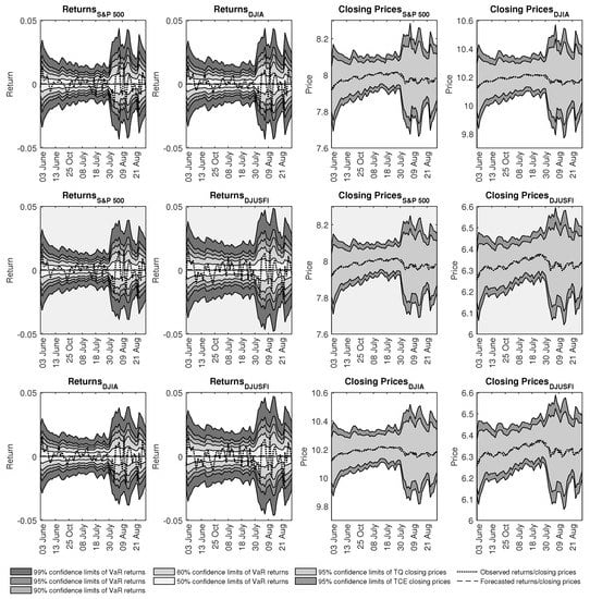
Figure 4.
One-day-ahead VaR forecasts of returns (left 2 panels) and closing prices (right 2 panels) at varying levels for return series using two-stage MCARR-return model with S&P 500, DJIA and DJUSFI indices from 3 June 2019 to 30 August 2019.
Specifically, the number of VaR violations should follow a binomial distribution with h trials and success probability . Under the null hypothesis that this binomial model is true, the observed proportion should agree with the expected proportion . The forecast performance measures for one-day-ahead VaR forecasts using the best fit models are evaluated using the KUC test of [38] with the likelihood ratio (LR) test statistic given as
which is asymptotically chi-squared () distributed with one degree of freedom. The p-value of KUC test indicates whether there is sufficient evidence to reject the null hypothesis for the risk level .
As an alternative, [39] proposed an independent (CI) test which measures the dependency between consecutive days. The LR test statistic can be expressed as
where is the number of periods that have no failures followed by a period with no failures, is the number of periods that have failures followed by a period with no failures, is the number of periods with no failures followed by a period with failures, is the number of periods with failures followed by a period with failures, is the probability of having a failure on period t, is the probability of having a failure on period t given no failure on period , and the probability of having a failure on period t given a failure on period .
The test statistics and p-values of KUC and CI tests are respectively reported in Table 7 and Table 8. The p-values of these tests show insufficient evidence to reject the null hypotheses of VaR model at 5% level confirming the accuracy of VaR forecasts.
Table 7.
Forecast performance measures of the test statistic and p-value of KUC test for one-day-ahead VaR return forecasts at the lower and upper risk levels 0.005, 0.025 and 0.05 using the best two-stage MCARR-return model with volatility forecasts from MCARR(1,1,0), MCARR(1,1,1) and MCARR(1,1,0) models for the S&P 500, DJIA and DJUSFI indices. The subscripts in MCARR(1,1,0) and MCARR(1,1,1) for some and refer to i and j data pair.
Table 8.
Forecast performance measures of the test statistic and p-value of CI test for one-day-ahead VaR return forecasts at the lower and upper risk levels 0.005, 0.025 and 0.05 using the best two-stage MCARR-return model with volatility forecasts from MCARR(1,1,0), MCARR(1,1,1) and MCARR(1,1,0) models for the S&P 500, DJIA and DJUSFI indices. The subscripts in MCARR(1,1,0) and MCARR(1,1,1) for some and refer to i and j data pair.
Table 9 displays two loss functions, root mean squared forecast error (RMSFE) and mean absolute forecast error (MAFE), for the closing price forecasts. For S&P 500 index, the univariate CARR(1,1,1) model provides the smallest RMSFE and MAFE showing independence from other indices. For DJIA and DJUSFI indices, MCARR(1,1,0) model paired with S&P 500 index gives the smallest RMSFE and MAFE showing dependency with S&P 500 and absence of leverage effect in the volatility measures.
Table 9.
RMSFE and MAFE loss functions for out-of-sample closing price forecasts using the two-stage CARR-return and MCARR-return models. Volatilities are estimated from both CARR and MCARR models for each of the S&P 500, DJIA and DJUSFI index series. The stage-two return models in the two-stage CARR-return and MCARR-return models use constant mean function and Student-t and MVT error distributions, respectively.
5. Conclusions
In this paper, we propose the two-stage MCARR-return models to study returns, volatilities and correlation of market indices. We provide details of applying the models through analysing S&P 500, DJIA and DJUSFI indices with 1-minute sampling frequency. In these empirical studies, we begin with proposing the SRPK volatility measures and applying the measures to MCARR models with MLN distributed errors for each pair of indices in the first stage. We consider two models, MCARR(1,1,0) and MCARR(1,1,1) in which the mean function has no leverage effect and leverage effect, respectively. We explore ways to simplify the coefficient matrices in the mean function to reduce the number of parameters. In the second stage, the volatility and covariance estimates or forecasts from the best performed MCARR model are imported to the multivariate return models to estimate the returns. The errors of these return models are assigned the MVT distribution. We compare the in-sample fits of volatilities and returns using LL and AIC. For returns, we compare the performances of the two-stage MCARR(1,1,0)-return and MCARR(1,1,1)-return models with MVT error distribution to BEKK-GARCH(1,1) models with MVN and MVT distributions. The results from each pair of in-sample fits show that the best two-stage MCARR-return models outperform all BEKK-GARCH models. The best two-stage MCARR-return model is the MCARR(1,1,0)-return model with a constant mean function for two pairs of indices and the MCARR(1,1,1)-return model with constant mean function for one pair of indices.
Then these best models are applied to provide one-day-ahead volatility and return forecasts for 64 days. The predictive performances of volatility forecasts are evaluated using RL functions with SRCO measure chosen to be the proxy for true volatility. The one-day-ahead VaR and CVaR forecasts of returns at lower and upper risk levels 0.005, 0.025, 0.05, and one-day-ahead TQ and TCE forecasts of closing prices at lower and upper risk levels 0.025 using the best performed model are obtained. The p-values of KUC and CI tests show insufficient evidences to reject the null hypotheses of the VaR model at 5% level across all risk levels, confirming the accuracy of the VaR forecasts. In summary, the proposed two-stage MCARR-return models can capture the persistence, volatility spillover and leverage effects of the volatility dynamics, cross dependence between asset returns, and leptokurtic return distribution. These effects are all estimated to be significant in our data.
However, there are a few limitations of our study. Firstly, intraday prices information is required to measure the variance of the sum of a pair of returns using any volatility measure such as the SRPK that we adopt. Daily prices fail to measure the variance of the sum of two returns as the maximum of the sum is not the sum of each maximum unless the sum and, hence, each return are continuously observed. Hence, the dynamics of the sum of returns process need to be estimated using realised volatility based on more intra-period observations as explained in (12) and (13). On the other hand, collecting high frequency intraday price information is possible from many platforms. Apart from SRPK, there are other more efficient volatility measures such as scaled realised Garman–Klass and scaled realised Rogers–Satchell measures since these measures apply intraday open-close apart from high-low information.
Secondly, the MCARR model models the covariance indirectly through modelling the variance of pairwise sum of returns. This is less efficient as features of covariance may be different from those in the variance of pairwise sum. For future research, one may consider modelling directly the time series of variance-covariance matrix measures using (8) as one possible measure. Then can be assigned to the conditional Wishart distribution [26] with the mean matrix adopting a structure similar to (35) for the BEKK-GARCH model which contains short-term persistence matrix and long-term persistence matrix . Then in (28) with can be estimated using . Moreover, can also adopt a structure similar to DCC-GARCH which models variance and correlation matrix simultaneously. This model adopts range information more directly than the range-based MGARCH models. The Wishart model ensures positive-definite covariance matrices without imposing parameter constraints. The model can be estimated easily using maximum likelihood method with closed-form pdf. This is an interesting field for the analysis of moderate dimensional variance-covariance matrix processes.
However, the MCARR and Wishart models cannot solve the curse of dimensionality problem. As the number of assets increases, the number of parameters may explode, causing problems of convergence and parameter instabilities. To reduce the number of parameters, we suggest to impose some constraints such as symmetric coefficient matrices for the short and long term persistence and diagonal coefficient matrices for the leverage effect. Another approach is to use factor model for time series [42]. Moreover, machine learning models can handle high dimensional data without imposing any distributional or structural assumptions. Convolutional neural network (CNN) and recurrent neural network (RNN) are the most common types of neural network in capturing image data and sequential data, respectively. Ref. [43] used GARCH and RNN models to forecast Bitcoin’s return volatility and VaR. They showed that RNN model is more sensitive and responds more quickly to volatility change than the traditional financial time series models. Ref. [44] proposed a Convolutional Long Short Term Memory neural network (CLSTM-NN) to handle the high dimensional realised covariance matrices consistently. However, although CLSTM-NN can demonstrate its excellent forecasting ability, specific features that drive the covariance process seems to be hidden in a black-box. This limitation is particularly unappealing when the dynamics of the covariance process is the focus of the model. Hence, future research can be directed to explore some hybrid statistical and neural network models that can overcome the curse of dimensionality problem and preserve some model interpretability.
Author Contributions
Conceptualization, K.H.N. and J.S.-K.C.; Methodology, S.K.T., K.H.N. and J.S.-K.C.; Software, S.K.T.; Validation, S.K.T., K.H.N. and J.S.-K.C.; Formal analysis, S.K.T.; Investigation, S.K.T., K.H.N. and J.S.-K.C.; Data curation, S.K.T.; Writing—original draft, S.K.T., K.H.N. and J.S.-K.C.; Writing—review & editing, S.K.T., K.H.N. and J.S.-K.C.; Supervision, K.H.N. and J.S.-K.C. All authors have read and agreed to the published version of the manuscript.
Funding
This research received no external funding.
Institutional Review Board Statement
Not applicable.
Informed Consent Statement
Not applicable.
Data Availability Statement
The data are based on Standard and Poor 500, Dow Jones Industrial Average and Dow Jones United States Financial Service Indices.
Acknowledgments
The authors would like to thank the editors and anonymous reviewers for their valuable and constructive comments to improve the quality of the paper.
Conflicts of Interest
The authors declare no conflict of interest.
References
- Bollerslev, T. Generalized autoregressive conditional heteroskedasticity. J. Econom. 1986, 31, 307–327. [Google Scholar] [CrossRef]
- Taylor, S.J. Modelling Financial Time Series; John Wiley & Sons: Chichester, UK, 1986. [Google Scholar]
- Parkinson, M. The extreme value method for estimating the variance of the rate of return. J. Bus. 1980, 53, 61–65. [Google Scholar] [CrossRef]
- Garman, M.B.; Klass, M.J. On the estimation of security price volatilities from historical data. J. Bus. 1980, 53, 67–78. [Google Scholar] [CrossRef]
- Rogers, L.C.G.; Satchell, S.E. Estimating variance from high, low and closing prices. Ann. Appl. Probab. 1991, 1, 504–512. [Google Scholar] [CrossRef]
- Yang, D.; Zhang, Q. Drift independent volatility estimation based on high, low, open, and close prices. J. Bus. 2000, 73, 477–492. [Google Scholar] [CrossRef]
- Andersen, T.G.; Bollerslev, T. Answering the skeptics: Yes, standard volatility models do provide accurate forecasts. Int. Econ. Rev. 1998, 39, 885–905. [Google Scholar] [CrossRef]
- Christensen, K.; Podolskij, M. Realized range-based estimation of integrated variance. J. Econom. 2007, 141, 323–349. [Google Scholar] [CrossRef]
- Martens, M.; Van Dijk, D. Measuring volatility with the realized range. J. Econom. 2007, 138, 181–207. [Google Scholar] [CrossRef]
- Gerlach, R.; Wang, C. Forecasting risk via realized GARCH, incorporating the realized range. Quant. Financ. 2016, 16, 501–511. [Google Scholar] [CrossRef]
- Chou, R.Y. Forecasting financial volatilities with extreme values: The conditional autoregressive range (CARR) model. J. Money Credit Bank. 2005, 37, 561–582. [Google Scholar] [CrossRef]
- Chan, J.S.K.; Ng, K.H.; Ragell, R. Bayesian return forecasts using realised range and asymmetric CARR model with various distribution assumptions. Int. Rev. Econ. Financ. 2019, 61, 188–212. [Google Scholar] [CrossRef]
- Tan, S.K.; Chan, J.S.K.; Ng, K.H. Modelling and forecasting stock volatility and return: A new approach based on quantile Rogers–Satchell volatility measure with asymmetric bilinear CARR model. Stud. Nonlinear Dyn. Econom. 2022, 26, 437–4774. [Google Scholar] [CrossRef]
- Bauwens, L.; Laurent, S.; Rombouts, J.V.K. Multivariate GARCH models: A survey. J. Appl. Econom. 2006, 21, 79–109. [Google Scholar] [CrossRef]
- Korkie, B. Corrections for trading frictions in multivariate returns. J. Financ. 1989, 44, 1421–1434. [Google Scholar] [CrossRef]
- Bollerslev, T.; Engle, R.F.; Wooldridge, J.M. A capital asset pricing model with time-varying covariances. J. Political Econ. 1988, 96, 116–131. [Google Scholar] [CrossRef]
- Engle, R.F.; Kroner, K.F. Multivariate simultaneous generalized ARCH. Econom. Theory 1995, 11, 122–150. [Google Scholar] [CrossRef]
- Engle, R.F. Dynamic conditional correlation: A simple class of multivariate generalized autoregressive conditional heteroskedasticity models. J. Bus. Econ. Stat. 2002, 20, 339–350. [Google Scholar] [CrossRef]
- Harvey, A.; Ruiz, E.; Shephard, N. Multivariate stochastic variance models. Rev. Econ. Stud. 1994, 61, 247–264. [Google Scholar] [CrossRef]
- Fernandes, M.; de Sá Mota, B.; Rocha, G. A multivariate conditional autoregressive range model. Econ. Lett. 2005, 86, 435–440. [Google Scholar] [CrossRef]
- Fiszeder, P. Low and high prices can improve covariance forecasts: The evidence based on currency rates. J. Forecast. 2018, 37, 641–649. [Google Scholar] [CrossRef]
- Fiszeder, P.; Fałdziński, M. Improving forecasts with the co-range dynamic conditional correlation model. J. Econ. Dyn. Control. 2019, 108, 103736. [Google Scholar] [CrossRef]
- Molnár, P. High-low range in GARCH models of stock return volatility. Appl. Econ. 2016, 48, 4977–4991. [Google Scholar] [CrossRef]
- Fiszeder, P.; Fałdziński, M.; Molnár, P. Range-based DCC models for covariance and value-at-risk forecasting. J. Empir. Financ. 2019, 54, 58–76. [Google Scholar] [CrossRef]
- Chou, R.Y.; Wu, C.C.; Liu, N. Forecasting time-varying covariance with a range-based dynamic conditional correlation model. Rev. Quant. Financ. Account. 2009, 33, 327–345. [Google Scholar] [CrossRef]
- Wishart, J. The generalised product moment distribution in samples from a normal multivariate population. Biometrika 1928, 20, 32–52. [Google Scholar] [CrossRef]
- Konno, Y. A note on estimating eigenvalues of scale matrix of the multivariate F-distribution. Ann. Inst. Stat. Math. 1991, 43, 157–165. [Google Scholar] [CrossRef]
- Kumar, D.; Maheswaran, S. A new approach to model and forecast volatility based on extreme value of asset prices. Int. Rev. Econ. Financ. 2014, 33, 128–140. [Google Scholar] [CrossRef]
- Tan, S.K.; Ng, K.H.; Chan, J.S.K.; Mohamed, I. Quantile range-based volatility measure for modelling and forecasting volatility using high frequency data. North Am. J. Econ. Financ. 2019, 47, 537–551. [Google Scholar] [CrossRef]
- Chou, R.Y.; Liu, N. The economic value of volatility timing using a range-based volatility model. J. Econ. Dyn. Control. 2010, 34, 2288–2301. [Google Scholar] [CrossRef]
- Auer, B.R. How does Germany’s green energy policy affect electricity market volatility? An application of conditional autoregressive range models. Energy Policy 2016, 98, 621–628. [Google Scholar] [CrossRef]
- Chen, C.W.S.; Gerlach, R.; Lin, E.M.H. Volatility forecasting using threshold heteroskedastic models of the intra-day range. Comput. Stat. Data Anal. 2008, 52, 2990–3010. [Google Scholar] [CrossRef]
- Chan, J.S.K.; Lam, C.P.Y.; Yu, P.L.H.; Choy, S.T.B.; Chen, C.W.S. A Bayesian conditional autoregressive geometric process model for range data. Comput. Stat. Data Anal. 2012, 56, 3006–3019. [Google Scholar] [CrossRef]
- Ng, K.H.; Peiris, S.; Chan, J.S.K.; Allen, D.; Ng, K.H. Efficient modelling and forecasting with range based volatility models and its application. North Am. J. Econ. Financ. 2017, 42, 448–460. [Google Scholar] [CrossRef]
- Patton, A.J. Volatility forecast comparison using imperfect volatility proxies. J. Econom. 2011, 160, 246–256. [Google Scholar] [CrossRef]
- Jorion, P. Risk2: Measuring the risk in value at risk. Financ. Anal. J. 1996, 52, 47–56. [Google Scholar] [CrossRef]
- Artzner, P.; Delbaen, F.; Eber, J.M.; Heath, D. Coherent measures of risk. Math. Financ. 1999, 9, 203–228. [Google Scholar] [CrossRef]
- Kupiec, P.H. Techniques for verifying the accuracy of risk measurement models. J. Deriv. 1995, 3, 73–84. [Google Scholar] [CrossRef]
- Christoffersen, P.F. Evaluating interval forecasts. Int. Econ. Rev. 1998, 39, 841–862. [Google Scholar] [CrossRef]
- Ślepaczuk, R.; Zakrzewski, G. High-Frequency and Model-Free Volatility Estimators; Working Papers No. 13/2009(23); Faculty of Economic Sciences, University of Warsaw: Warsaw, Poland, 2009. [Google Scholar]
- Christoffersen, P.F. Elements of Financial Risk Management; Academic Press: San Diego, CA, USA, 2003. [Google Scholar]
- Eichler, M.; Motta, G.; Von Sachs, R. Fitting dynamic factor models to non-stationary time series. J. Econom. 2011, 163, 51–70. [Google Scholar] [CrossRef]
- Shen, Z.; Wan, Q.; Leatham, D.J. Bitcoin return volatility forecasting: A comparative study between GARCH and RNN. J. Risk Financ. Manag. 2021, 14, 337. [Google Scholar] [CrossRef]
- Fang, Y.; Yu, P.L.; Tang, Y. CNN-based realized covariance matrix forecasting. arXiv 2021, arXiv:2107.10602. [Google Scholar]
Disclaimer/Publisher’s Note: The statements, opinions and data contained in all publications are solely those of the individual author(s) and contributor(s) and not of MDPI and/or the editor(s). MDPI and/or the editor(s) disclaim responsibility for any injury to people or property resulting from any ideas, methods, instructions or products referred to in the content. |
© 2022 by the authors. Licensee MDPI, Basel, Switzerland. This article is an open access article distributed under the terms and conditions of the Creative Commons Attribution (CC BY) license (https://creativecommons.org/licenses/by/4.0/).