Numerical Research of Dynamical Behavior in Engineering Applications by Using E–E Method

Abstract

In this research, a general numerical setting has been developed by finite volume approaching for the Eulerian–Eulerian method under OpenFOAM to provide an efficient reference for industrial bubbly flows having various geometrical characteristics under different conditions. Nine different test cases were selected from chemical, nuclear, bio-processing and metallurgical engineering. We compared the predicted results with experimental findings, and the comparison proved that our implementation is correct. The numerical result has good agreement with the experimental result in most testing cases. From the analysis, we found that turbulent dispersion and drag forces were of critical importance and had to be considered in simulations. The turbulent dispersion took into account the turbulence effect, and the drag forces considered two-way coupling and ensured the good position of the Eulerian–Eulerian equations. Wall lubrication and lift forces had to be considered to solve phase fraction accumulation near walls, especially for aspect ratio pipe flows. Under other conditions, lateral forces could be neglected without any problem.

1. Introduction

Gas-liquid flows have wide uses and can be simulated by different models, such as Eulerian–Lagrangian (E–L) and Eulerian–Eulerian (E–E) methods and the direct method, which is also called multi-phase direct numerical simulation (DNS). Each fluid phase in the E–E method [1,2,3,4,5,6,7,8,9] is assumed to be a continuum in given computational domains capable of being interpenetrated with other fluid phases. A variety of methods for averaging (including ensemble or volume averaging) were applied for obtaining basic governing equations. In the E-L approach [10,11,12,13], the continuous phase was processed in the Eulerian framework while individual bubble motions were simulated through the solution of the equation of force balance. Bubbles trajectories were calculated in control volume and the average values were reported. Navier–Stokes equations were directly applied in multi-phase DNS [14,15,16,17,18,19], and phase interface topology was established as a part of the solution. No other assumptions were considered in the modelling. For resolving wide spatial and temporal scale ranges, DNS needs high resolutions. These scale ranges depended on interface topologies, such as dispersed particle sizes, and fluid motion, such as eddies involved in turbulent motions. Solving these scales requires high computational costs in terms of both execution time and memory size. Hence, DNS is limited to low bubbles/particles and Reynolds numbers.

Thanks to computational economics, many works have used the E–E method to simulate gas-liquid flows. However, as a macroscopic method, the E–E method (1) requires constitutive models (e.g., the solid-phase stress model); (2) requires models to address the momentum and energy exchange terms (e.g., the drag model); and (3) loses the characteristic feature for those scales, which is much smaller than the mesh resolution. To obtain reasonable results, suitable sub-models and parameters should be adjusted. Moreover, the observed flow field is also different for the gas-liquid flows in different industries. For example, bubble columns are quite common in the chemical engineering industry. A bubble column liquid flow field tends to form a circulation model due to the movement of the bubbles, which is generally called “Gulf stream” or “cooling tower” flow regimes. In nuclear engineering, the phase fraction of the bubbles in a vertical upward pipe shows a wall peak due to the lateral movement of the small bubbles [20,21,22]. Without loss of generality, the ability of the E–E method to capture typical flow field information was verified. However, the amount of work needs to be studied for the sub-models, especially for the momentum interfacial exchange models.

The drag force and the buoyancy force, as the most important momentum interfacial exchange forces, determine the bubble terminal velocity and address the coupling of continuous and dispersed phases. Lift and wall lubrication forces address bubble lateral movements. It is of critical importance to correctly describe the wall and lift coefficients when modelling this transversal force. The turbulence dispersion force pushes bubbles from higher to lower phase fraction areas because of continuous phase pressure variation, which is not solved at the meso-scale. Picardi et al. [23] reported the mesh resolution is critical for the predictions by the E–E method. It has also been shown by Panicker et al. [24] and Vaidheeswaran and Lopez de Bertodano [25] that the addition of a dispersion term ensures the hyperbolicity of the partial differential equation (PDE) and prevents the non-physical instabilities in the predicted multiphase flows upon grid refinement.

Gas-liquid flows have also gained much attention from the marine engineering field since it has been found that micro-air bubbles injected into water can reduce the friction drag of marine vehicles, such as submarines and ships. Mohanarangam et al. [26] simulated the micro-bubble drag reduction on a flat plate in water based on the E–E method with a population balance model and showed a good agreement on the drag reduction between computational fluid dynamics (CFD) and model test results. Zhang et al. [27] showed a Euler-–Lagrange simulation on the bubble drag reduction on a flat plate, in which they adopted a two-coupled E-L method, and the bubble-turbulence interaction is analyzed. In Zhao et al. [28], the drag reduction of an axisymmetric body was numerically studied based on OpenFOAM, in which the effect of air flow rate and bubble size are discussed.

Despite general agreement in the literature on the requirement of incorporating drag into bubble column models, many works admit that there is still a lack of consensus on other forces to be applied at best in communities [29], which gave the motivation of this research. The purpose of the present research is to simulate a large amount of gas-liquid flows with different force closure combinations to investigate their importance. Our contribution is to provide a general numerical configuration for the E–E method, capable of providing proper results for bubbly flows in different industries.

2. Description of Models

Two Navier–Stokes equation sets in the Eulerian framework were ensemble-averaged, and inter-phase phenomena and turbulence effects were considered based on closure models. Mass conservation for phases a and b could be stated as [30]:

$$\frac{\partial \left({\alpha }_{\mathrm{a}}{\rho }_{\mathrm{a}}\right)}{\partial t}+\nabla ·\left({\alpha }_{\mathrm{a}}{\rho }_{\mathrm{a}}{\mathbf{U}}_{\mathrm{a}}\right)=0,$$

(1)

$$\frac{\partial \left({\alpha }_{\mathrm{b}}{\rho }_{\mathrm{b}}\right)}{\partial t}+\nabla ·\left({\alpha }_{\mathrm{b}}{\rho }_{\mathrm{b}}{\mathbf{U}}_{\mathrm{b}}\right)=0,$$

(2)

where ${\alpha }_{\mathrm{a}}$ and ${\alpha }_{\mathrm{b}}$ are phase fractions, ${\rho }_{\mathrm{a}}$ and ${\rho }_{\mathrm{b}}$ are densities, and ${\mathbf{U}}_{\mathrm{a}}$ and ${\mathbf{U}}_{\mathrm{b}}$ are the average velocities of phases a and b, respectively. ${\mathbf{U}}_{\mathrm{a}}$ and ${\mathbf{U}}_{\mathrm{b}}$ were obtained through the solution of corresponding phase momentum equations [30]:

$$\frac{\partial \left({\alpha }_{\mathrm{a}}{\rho }_{\mathrm{a}}{\mathbf{U}}_{\mathrm{a}}\right)}{\partial t}+\nabla ·\left({\alpha }_{\mathrm{a}}{\rho }_{\mathrm{a}}{\mathbf{U}}_{\mathrm{a}}{\mathbf{U}}_{\mathrm{a}}\right)-\nabla ·\left({\alpha }_{\mathrm{a}}{\rho }_{\mathrm{a}}{\mathbf{Ø}}_{\mathrm{a}}\right)=-{\alpha }_{\mathrm{a}}\nabla p_{\mathrm{a}}+{\alpha }_{\mathrm{a}}{\rho }_{\mathrm{a}}\mathbf{g}-\mathbf{M},$$

(3)

$$\frac{\partial \left({\alpha }_{\mathrm{b}}{\rho }_{\mathrm{b}}{\mathbf{U}}_{\mathrm{b}}\right)}{\partial t}+\nabla ·\left({\alpha }_{\mathrm{b}}{\rho }_{\mathrm{b}}{\mathbf{U}}_{\mathrm{b}}{\mathbf{U}}_{\mathrm{b}}\right)-\nabla ·\left({\alpha }_{\mathrm{b}}{\rho }_{\mathrm{b}}{\mathbf{Ø}}_{\mathrm{b}}\right)=-{\alpha }_{\mathrm{b}}\nabla p_{\mathrm{b}}+{\alpha }_{\mathrm{b}}{\rho }_{\mathrm{b}}\mathbf{g}+\mathbf{M},$$

(4)

where $p_{\mathrm{a}}$ and $p_{\mathrm{b}}$ are effective Reynolds stress tensors, ${\mathbf{Ø}}_{\mathrm{a}}$ and ${\mathbf{Ø}}_{\mathrm{b}}$ are the pressure for each phase, $\mathbf{M}$ is the interfacial force exchange term, and $\mathbf{g}$ is the vector of gravitational acceleration. $\mathbf{M}$ can be divided into axial drag force ${\mathbf{M}}_{\mathrm{drag}}$, the wall lubrication force ${\mathbf{M}}_{\mathrm{wall}}$ driving bubbles away from walls [31], the lateral lift force ${\mathbf{M}}_{\mathrm{lift}}$ acting perpendicular to the relative motion directions of two phases [32], and the turbulent dispersion force ${\mathbf{M}}_{\mathrm{turb}}$ resulting from liquid velocity turbulent fluctuations [33]. Specially, drag force was obtained as below:

$${\mathbf{M}}_{\mathrm{drag}}=\frac{3}{4}{\alpha }_{\mathrm{a}}{\rho }_{\mathrm{b}}{C}_{\mathrm{D}}\frac{1}{d_{\mathrm{a}}}\left|{\mathbf{U}}_{\mathrm{b}}-{\mathbf{U}}_{\mathrm{a}}\right|\left({\mathbf{U}}_{\mathrm{b}}-{\mathbf{U}}_{\mathrm{a}}\right),$$

(5)

where $d_{\mathrm{a}}$ is the phase a diameter and $C_{\mathrm{D}}$ is drag force coefficient. Lift force was obtained as [34]:

$${\mathbf{M}}_{\mathrm{lift}}={\alpha }_{\mathrm{b}}{C}_{\mathrm{L}}{\rho }_{\mathrm{a}}{\mathbf{U}}_{\mathrm{r}}\times \left(\nabla \times {\mathbf{U}}_{\mathrm{b}}\right),$$

(6)

where ${\mathbf{U}}_{\mathrm{r}}$ is the relative velocity calculated as ${\mathbf{U}}_{\mathrm{b}}-{\mathbf{U}}_{\mathrm{a}}$, and $C_{\mathrm{L}}$ is the lift force coefficient. The wall lubrication force was obtained as [31]:

$${\mathbf{M}}_{\mathrm{wall}}=C_{\mathrm{wall}}{\rho }_{\mathrm{b}}{\alpha }_{\mathrm{a}}{\left|{\mathbf{U}}_{\mathrm{r}}\right|}^2·\mathbf{n},$$

(7)

where $C_{\mathrm{wall}}$ is the force coefficient of wall lubrication. Turbulence dispersion force was obtained as [33]:

$${\mathbf{M}}_{\mathrm{turb}}=C_{\mathrm{T}}{\rho }_{\mathrm{b}}{k}_{\mathrm{b}}\nabla {\alpha }_{\mathrm{a}},$$

(8)

where $C_{\mathrm{T}}$ is the turbulence dispersion force coefficient. A comprehensive discussion of the E–E method is available in [35,36]. Readers are referred to our previous work [37] and the Appendix A for the finite volume discretization of the E–E method.

In the E–E method, liquid phase-bubble interactions are modelled by the momentum interfacial exchange forces in gas and liquid phase momentum equations. No general consensus has been obtained in scientific communities on the closures to be applied at best. Physically, the effect of these forces is reported in Figure 1. In a quiescent environment, the buoyancy force pushes the bubbles upward. On the other hand, the drag force tends to exert itself in the opposite direction of the bubble movement. The drag force direction is equivalent to that of relative velocity. In simplest cases, these two forces can reach a balance, and the velocity of the terminal bubble can be obtained.

Lift force is created because of shear in the liquid phase acting perpendicular to the direction of bubble rise. Its direction depends on the value of the sign of $C_{\mathrm{L}}$. Different models can be used, such as the constant lift coefficient model and the model developed by Tomiyama [32]. Experiments show that the movement of small and large bubbles is opposite, especially in pesudo-steady-state pipe flows. It can only be predicted by employing a non-constant lift coefficient. Thus, the lift force coefficient developed by Tomiyama is more reasonable. Moreover, the largest shear exists not only in the vicinity of no-slip walls, it may be also large when one phase was injected into another phase with high velocity. The wall lubrication force exists only near solid objects. It drives the bubbles away from walls, avoiding bubble accumulation, which is not observed in the experiments. It should be noted that this force exists only near the walls. Thus, the distance between the nearest wall and bubble should be calculated in the wall force model. A turbulent dispersion force acts on the phase fraction gradient. It can be seen as diffusion, and it accounts for the random bubble movement in turbulent flows. It was found in many works that prediction results obtained from the E–E method are highly mesh-dependent, and this was due to the mathematical characteristic of the E-E equations [24,25]. Including the turbulent dispersion force avoids the ill-posed problems and improves the stability of the E-E model.

A large number of force models were developed in the literature, and it is not possible to compare all of them with all tests conducted in this study. Therefore, unless stated intentionally, we employ the lift force model by Tomiyama et al. [32], classic drag model by Zuber and Ishii [38], wall force by Antal et al. [31] and the turbulent dispersion force by Loptez De Bertodano [33] in our simulations. The working flowchart is shown in Figure 2 and includes geometry preparation, mesh generation, simulation setup, run simulation, and post-processing. Since we focus on the validation between numerical results and experiments, readers are suggested to see the Appendix A for the discretization of the governing equations.

3. Test Cases

As mentioned before, due to the lack of ideal experimental methods with proper global and local measurement mixtures under various operational conditions required for comprehensive model validation, we considered several test cases with different geometries. Only by using a large number of test cases can we find general numerical settings. These test cases were selected from different works. The schematic representation of these test cases is reported in Figure 3. All of them were investigated by experiments which imply they are suitable benchmark test cases for numerical investigations. Moreover, they were observed with different features as listed as follows:

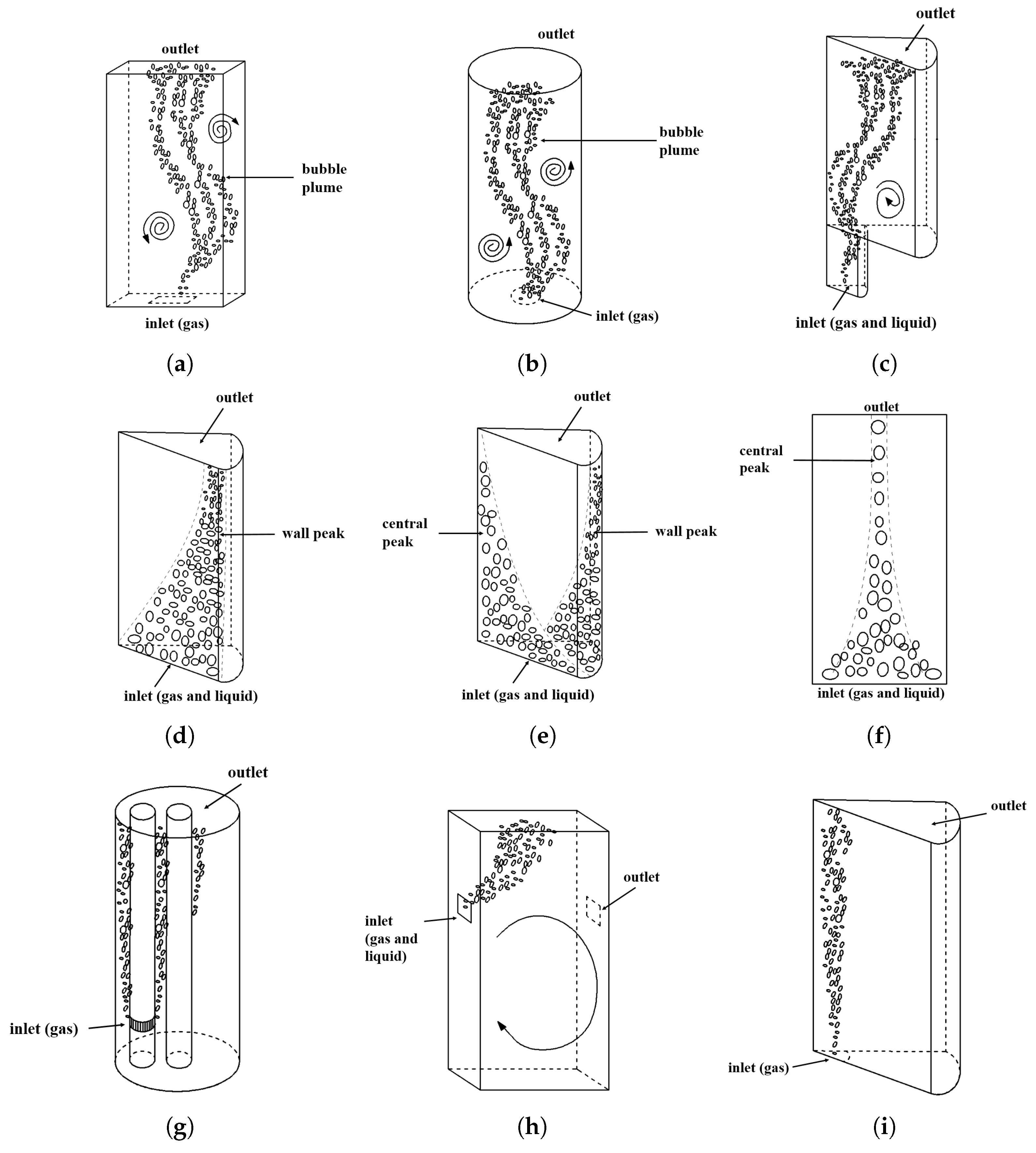
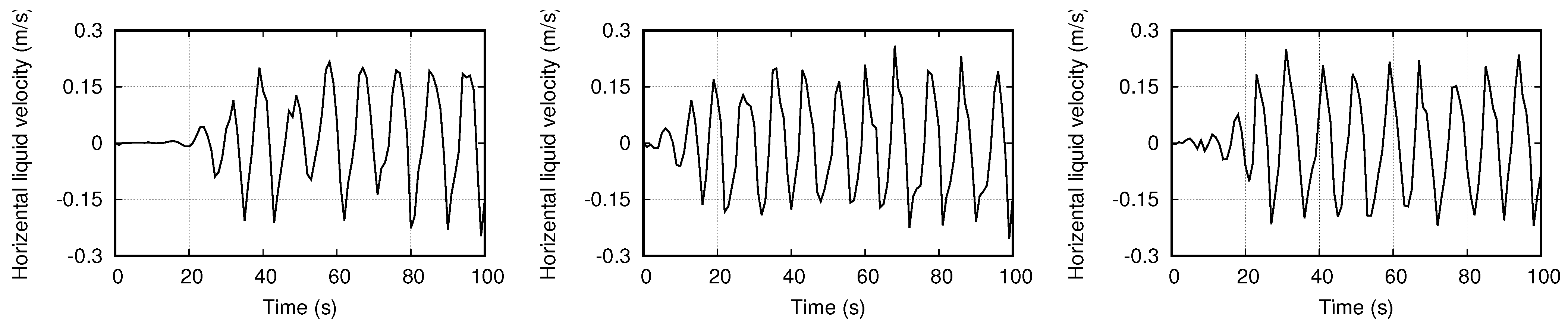
• Test case A.1: investigation of bubble plumes in a bubble column with rectangular shape developed by Díaz et al. [39]. The test setup consisted of a partially aerated bubble column with a width of 0.2 m, height of 1.8 m and depth of 0.04 m filled with tap water to 0.45 m under atmospheric pressure and room temperature while the air was fed through a sparger with eight concentric holes with a diameter of 1 mm and pitch 6 mm. This was a very interesting test case since liquid vortices created by bubble plumes were desirable for mixing and, consequently, accelerating all transport phenomena [40]. In addition, flow structures with unsteady liquid recirculations were typical phenomena of industrial bubble columns.
• Test case A.2: investigation of gas-liquid flows in an industrial bubble column proposed by McClure et al. [41], which was a partially aerated bubble column with a cylindrical shape of 0.19 m in diameter filled with water up to 1 m equipped with a multi-point sparger. The aspect ratio ($L/D$) was about 5. In the bio-processing industry, the bubble column height-to-diameter ratio typically ranges from 2 to 5 and is usually operated in the heterogeneous flow regime to speed up mass and heat transfer.
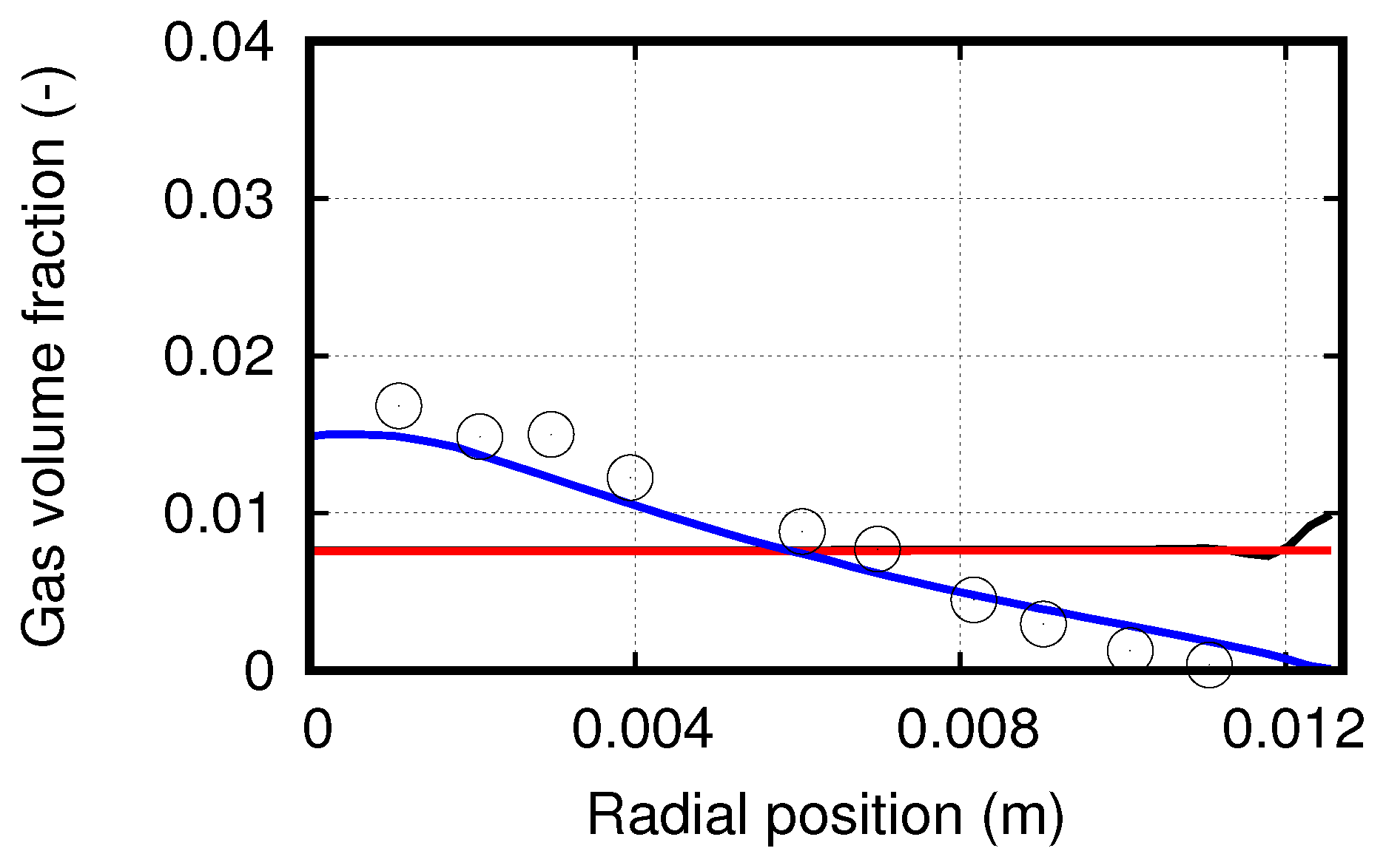
• Test case A.3: the test case investigated in this work was a bubbly air/water upward flow in a pipe with a sudden enlargement. The two sections of the pipe were 50 and 100 mm in diameter. The inlet phase fraction was known to have a wall peak. The main characteristic of this test was a large separation zone at the pipe bottom. This has been extensively applied for the verification and implimenttion of the E–E method [42,43,44,45].
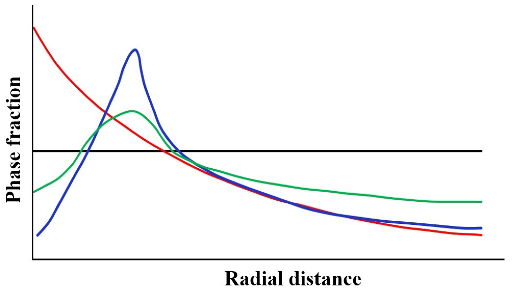
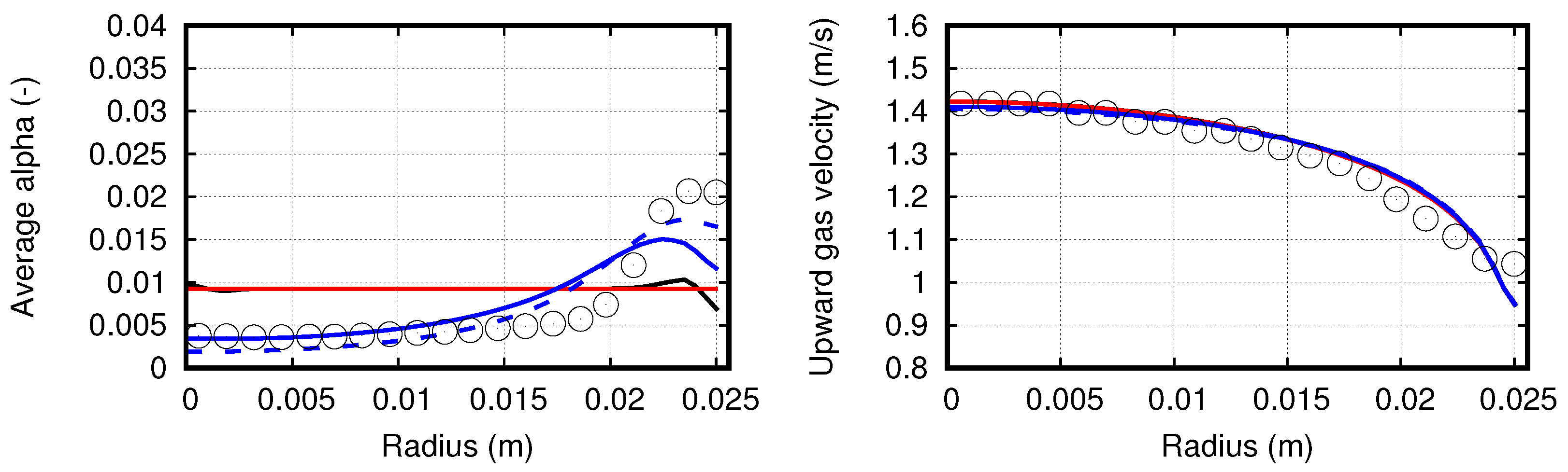
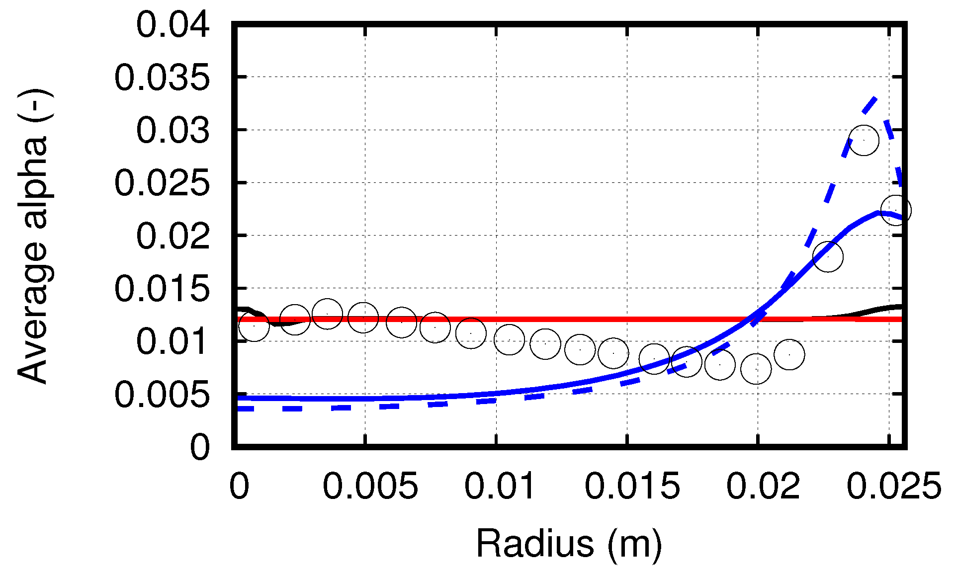
• Test case B.1: investigation of bubbly flow in a cylindrical pipe of Lucas et al. [46]. The mixture of the gas and liquid was injected from the bottom pipe of 0.0256 m in diameter and 3.53 m in height. In vertical upward flows, small bubbles moved towards the wall. A wall peak for gas phase fraction occurred at high $L/D$. Tomiyama et al. witnessed this phenomenon for individual bubbles [47]. For vertical co-current pipe flows, radial flow fields had symmetric stability over a long distance. Hence, this flow type is well investigated in terms of non-drag forces.
• Test case B.2: investigation of bubbly flows in a circular pipe developed by Banowski et al. [48]. The experiment comprised a vertical pipe with an inner diameter of 54.8 mm and a length of 6 m. The gas and liquid mixture was injected from the bottom. It was similar to the test case B.2. However, besides the typical wall peak formed due to the smaller bubbles’ movement, a double peak of the phase fraction can also be observed due to the existence of large bubbles since large bubbles tend to the centre.
• Test case B.3: investigation of bubbly flows in a rectangle pipe developed by Žun [49]. This test case was similar to test case B.3 with a slight difference of geometry. The mixture of the gas and liquid was injected from the bottom of a rectangle channel of 0.0254 m in length and 2 m in height. Only the central peak of the gas phase was witnessed.
• Test case B.4: investigation of the bubbly flow of Besagni et al. [50]. The gas-liquid flows in bubble columns with annular gaps and two non-regular internal pipes were investigated. It consisted of a non-pressurized vertical column with an inner diameter of 0.24 m and height of 5.3 m. It consisted of a non-pressurized vertical column with an inner diameter of 0.24 m and a height of 5.3 m. In the simulation domain, the height was limited to 5 m. Two internal pipes were arranged within the column: one positioned asymmetrically (0.075 m in external diameter) and the other positioned centrally (0.06 m in external diameter). The sparger was assumed to be a uniform surface with a cylindrical shape of 0.01 m in height located on the lateral inner pipe at a vertical position of 0.3 m from the domain bottom. The aspect ratio of the geometry was small. Due to the existence of the non-irregular components, the gas phase fraction distribution developed to be quite flattened, and no wall peak was observed in the experiments, even though it could be seen as a pipe flow.
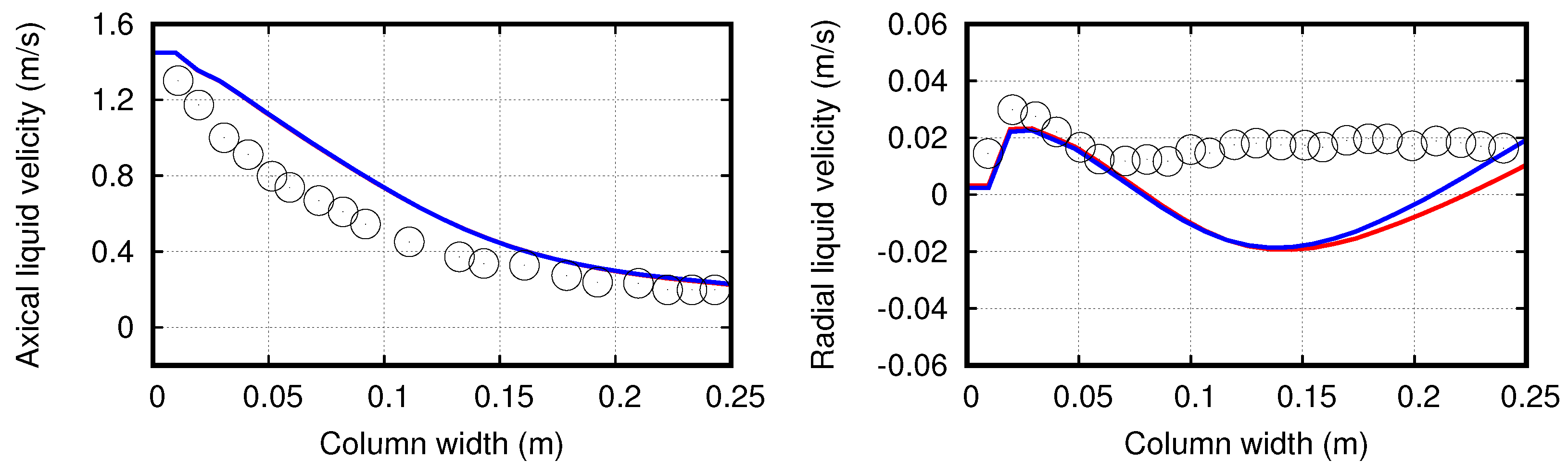
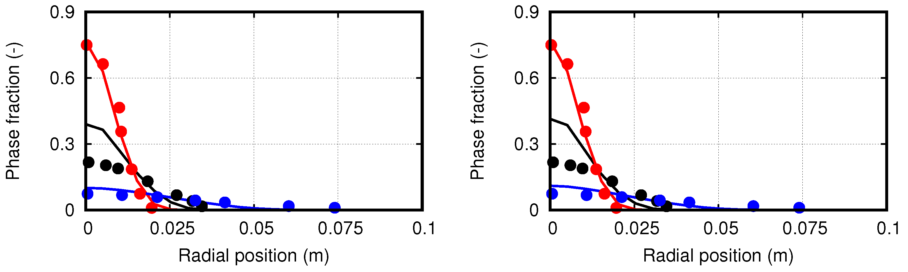
• Test case C.1: investigation of gas-liquid flows in a continuous casting mould of Iguchi and Kasai [51]. The geometry employed in this test case was quite different from previous ones. The gas and liquid were injected into a rectangular vessel of 0.3 m in length and 0.15 m in width. In the experiments, it was observed that larger bubbles were lifted towards the liquid surface because of buoyancy forces exerted on them, while smaller bubbles were pushed deep. Such a phenomenon is also known as phase segregation or poly-dispersity in other works, which was proven as a tough work for the E–E method.
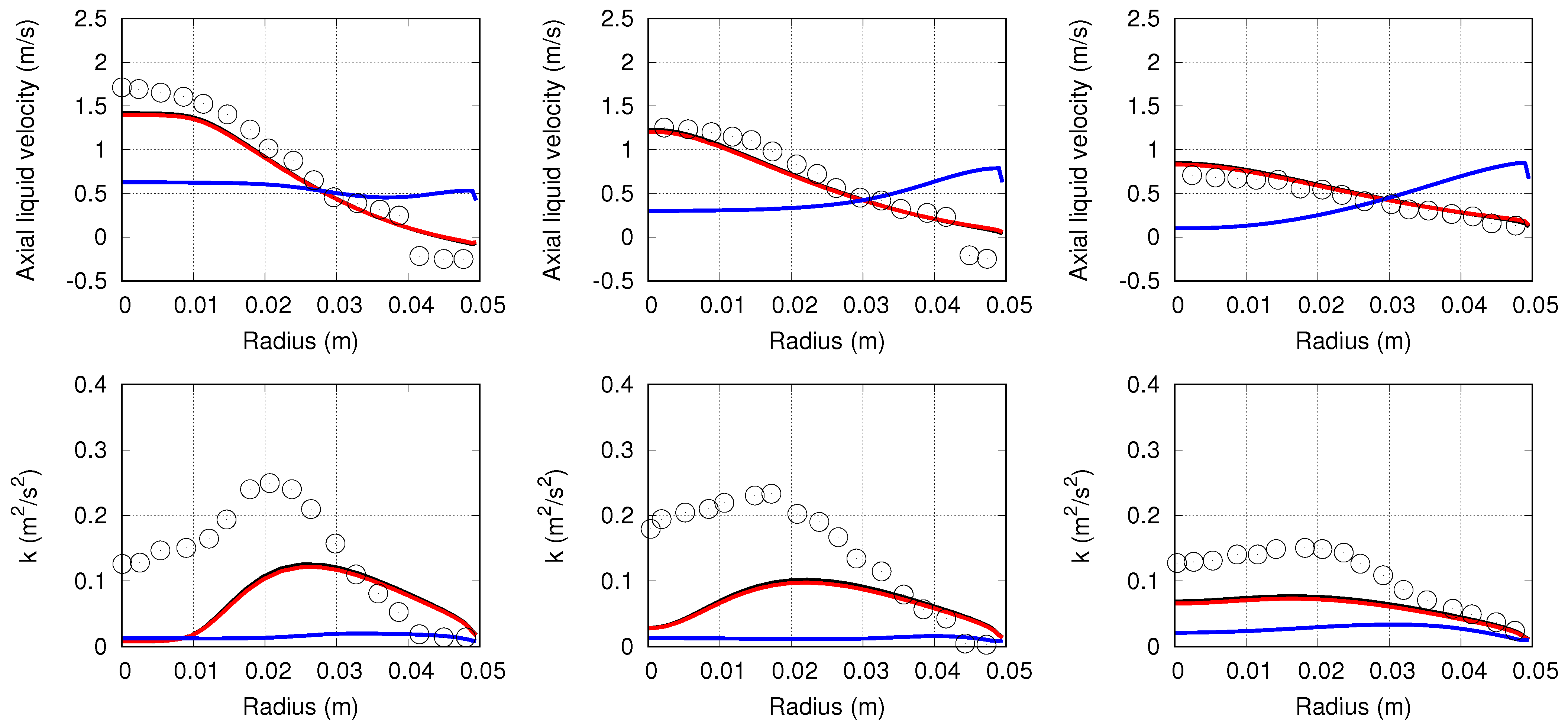
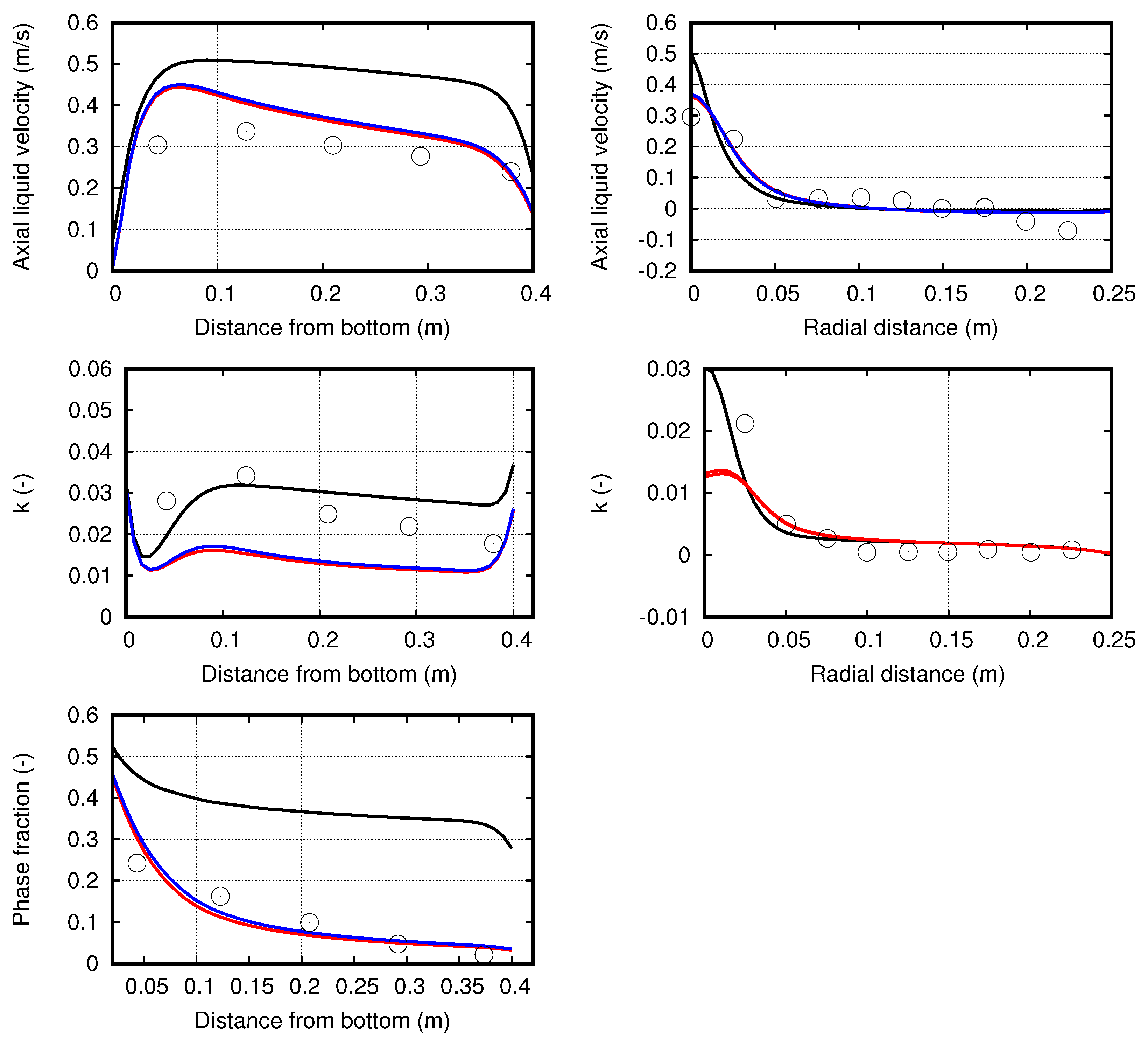
• Test case C.2: investigation of gas-liquid flows in a continuous casting mould of Sheng and Irons [52]. The gas phase was injected from the bottom of a vessel with a height of 0.76 m and a diameter of 0.5 m. In this test case, measured gas phase fraction distributions, turbulence fields, and velocities of gas/liquid in plume zones were employed for the validation of different turbulence models. It was observed to be a suitable test case to validate the multi-phase turbulence model against experimental data.

The reader may find these test cases are sorted by different groups. The bubble columns investigated in test cases A.1–A.3 are mainly encountered in chemical and bio-processing engineering. The aspect ratio of their geometry is small. They are usually used to speed up mixing and heat/mass transfer and are typically operated at a medium or high superficial velocity. A strong coupling between continuous and dispersed phases can be observed. The local phase fraction may be high. Meanwhile, the liquid flow in these bubble columns may be highly transient and full of chaos with large-scale vortices. The pipe flow investigated in test cases B.1–B.4 are mainly encountered in the nuclear engineering process. The aspect ratio of these pipes is relatively large. Different flow types exist depending on the gas flow rate. Dilute bubbly flows are found when operated at a low gas superficial velocity. In bubbly flows, the liquid flow is rather stable, and a steady state can be achieved. The shape of the phase fraction distribution develops gradually to a stable distribution along the pipe axial direction since the aspect ratio is quite large, which implies the gas phase has enough time to develop. The bubbly flows investigated in test cases C.1–C.2 are mainly encountered in metallurgical engineering. The scale of the gas-liquid reactor is the same as that employed in chemical engineering. The aspect ratio is also small. However, non-irregular design is quite common and the flow field is complex due to the existence of the complex geometry. Meanwhile, the small bubbles in the liquid phase, due to the phase segregation movement, are usually seen as impurities which need to be removed. At last, it should be stressed that although these test cases coming from different industries are full of different features, the core problem lies in gas-liquid flow investigations by the numerical method.

The computational grids employed in these test cases are shown in Figure 4. Here, 3D hexahedral cells were generated for test cases A.1, A.2 and C.1. Then, 2.5D axis-symmetric wedge cells were employed in test cases A.3, B.1, B.2 and C.2. Furthermore, 2D hexahedral cells were employed for test case B.3. Non-regular gambit-paving meshes were employed in test case B.4 because of the existence of non-regular geometries. Our grid independence investigation, though not shown herein for brevity, suggested that prediction results were insensitive to grid resolution. The base setup for these test cases is listed in

Table 1. Numerical configurations employed in test cases: $\psi$ is a generic variable, ${\nabla }^{\perp }$ is surface-normal gradient, and ${(\dots )}_f$ is the face interpolation operator. The number “1” indicates the compliance of the scheme with the definition of TVD scheme.

Term	Configuration
$\partial /\partial t$	Euler implicit
$\nabla \psi$	Gauss linear
$\nabla p$	Gauss linear
$\nabla ·\left(\psi \mathbf{U}\mathbf{U}\right)$	Gauss limitedLinearV 1;
$\nabla ·\left(\mathbf{U}\psi \right)$	Gauss limitedLinear 1
$\nabla ·\tau$	Gauss linear
${\nabla }^2\psi$	Gauss linear uncorrected
${\nabla }^{\perp }\psi$	Uncorrected
${\psi }_f$	Linear

and

Table 2. Solvers and related settings used in the test cases.

	Solver	Preconditioner	Rel. Tol.	Final Tol.
p	PCG	DIC	0.01	1 × 10${}^{-7}$
k	PBiCGStab	DILU	-	1 × 10${}^{-7}$
$\epsilon$	PBiCGStab	DILU	-	1 × 10${}^{-7}$

. In our preliminary investigations, such a numerical setup compromised stability and accuracy. Therefore, the remainder of the simulations in this study will utilize this base setup. The main boundary conditions are listed in

Table 3. Main boundary conditions adopted in the simulations.

Test Case	Operating Conditions
A.1	Superficial gas velocity: 0.0024 m/s Inlet liquid velocity: 0 m/s Bubble diameter: 0.00505 m
A.2	Superficial gas velocity: 0.16 m/s Inlet liquid velocity: 0 m/s Bubble diameter: 0.008 m
A.3	Inlet gas velocity: 1.87 m/s Inlet liquid velocity: 1.57 m/s Bubble diameter: 0.002 m
B.1	Superficial gas velocity: 0.0115 m/s Superficial liquid velocity: 1.0167 m/s Bubble diameter: 0.0048 m
B.2	Superficial gas velocity: 0.0151 m/s Superficial liquid velocity: 1.017 m/s Bubble diameter: 0.0046 m
B.3	Superficial gas velocity: 0.005 m/s Superficial liquid velocity: 0.43 m/s Bubble diameter: 0.006 m
B.4	Inlet gas velocity: 0.0087 m/s Inlet liquid velocity: 0 m/s Bubble diameter: 0.0042 m
C.1	Inlet gas velocity: 4 cm3/s Inlet liquid velocity: 5 L/s Bubble diameter: 0.005 m
C.2	Inlet gas velocity: 50 mL/s Inlet liquid velocity: 0 m/s Bubble diameter: 0.006 m
Gas velocity at walls: slip. Liquid velocity at walls: no-slip. k and $\epsilon$ at walls: wall function. Outlet: zero-gradient.

. Since many test cases were employed in this work, it is not possible to document all the settings for brevity. Readers are referred to the source code of the test cases for further details.

All the test cases were simulated by three basic settings. The first one only consisted of the drag force. The second one comprised turbulence dispersion and drag forces. The third one consisted of turbulence dispersion, drag, lift and wall forces. Our aim was to verify which force closure combination is able to provide the most universal settings.

4. Results and Discussion

4.1. Test Case A.1–A.3

In this section, the numerically predicted results for test cases A.1 to A.3 are investigated. The available experimental data and features are listed in

Table 4. Available experimental data and features of test cases A.1 to A.3.

Test Case	Exp. Data	Features	Pseudo-Steady-State
A.1	Plume oscillating period Gas holdup	Periodic flow field	No
A.2	Phase frac. distri.	High phase fraction	No
A.3	Upward liquid vel. Turb. kinetic energy	Stagnant vortex	Yes

. These test cases are common in chemical and bio-processing engineering. In test case 4, the gas phase was injected into the column at a relatively small superficial velocity. A “cooling tower” flow regime was formed due to the existence of a periodic large vortex. In test case A.2, the gas phase was injected into the cylinder column at high superficial velocities. The flow fields were highly transient and full of vortexes. In test case A.3, the gas phase was injected into a sudden enlargement pipe, and a steady-state stagnant vortex was formed at the pipe bottom. In experiments, the turbulence kinetic energy was monitored, which can be used to validate the turbulence model employed in the E–E method.

Figure 5 show the horizontal liquid velocity predicted by different force closure combination for test case A.1. It can be seen that all the force closure combinations can predict the periodic “Gulf-stream” phenomenon, which proves that the periodical vortex in the bubble column is not sensitive to the forced closure.

Table 5. Comparison of the gas holdup and POP predicted by different force closure combinations with experimental data for test case A.1.

	Drag Force	Drag & Dispersion Forces	Drag & Dispersion & Lift and Wall Forces	Exp.
Gas holdup	0.00613	0.0065	0.0075	0.0069
Gas holdup rel. error	−11%	−6%	+8%	-
POP	9.37	8.87	8.98	11.38
POP rel. error	−17%	−22%	−21%	-

shows the predicted gas holdup and the plume oscillation period (POP). Compared to experimental findings, POP predicted by all these force closure combinations was under-estimated. Findings could be improved by adjusting the turbulence model and yhe inclusion of the bubble-induced turbulence, as was shown in our previous work [37]. On the other hand, all these three force closure combinations can predict good results of gas holdup with errors smaller than 11%. When the turbulence dispersion force and wall forces were taken into account, gas holdup prediction was slightly improved. However, the addition of wall forces and turbulence dispersion forces cannot improve the results of POP. This could be due to the fact that the phase shear rate in this test case is too small to present differences, and the occurrence of POP (or the periodical vortex) is mainly because of the drag.

Figure 6 presents the averaged phase fractions predicted by different computational grids (left) and force closure combinations for test case A.2. It was witnessed that the phase fraction was highly dependent on the grid size and employed force models, and the difference is quite large. If only drag force was taken into account, the predicted phase fraction was accumulated at the center of the column since no lateral forces and diffusion force were used. If the turbulence dispersion force was included, the bubbles at the center of the column were diffused along the gradient of the phase fraction, and the bubble-accumulating problem was prevented. Although the predicted phase fraction was flattened, it was much better than the predicted results when only drag force was considered. Moreover, flattened phase fraction can be handled by using smaller turbulence dispersion force coefficients. The addition of the wall forces cannot improve the results. Instead, the wall forces predict a peak in the vicinity of the wall, which was not observed in the experiments.

Figure 7 presents predicted mean axial liquid velocities and the turbulent kinetic energy for test case A.3. It can be seen from the experimental data that the mean axial liquid velocities gradually decrease along the radius, and the distribution trend of TKE along the radius is to increase first and then decrease, reaching a peak at a radius of 0.02 m. It was observed that predicting the axial liquid velocity agrees well with experiments in both trend and magnitude when the turbulence dispersion and drag forces were considered. However, including wall forces cannot predict reasonable results. It was observed that predicting the axial liquid velocity agree well with experiments in both trend and magnitude when the turbulence dispersion and drag forces were considered. However, including wall forces cannot predict reasonable results. Meanwhile, accurately predicting turbulent kinetic energy was proven to be quite difficult in both trend and amplitude. Although the combination of turbulence dispersion and drag forces improves the results compared with that predicted by addition of the wall forces, the predicted turbulent kinetic energy was under-estimated. Further research is needed to quantify these errors and possibly employ a bubble-induced turbulence model to correct the deficiencies [53].

4.2. Test Case B.1–B.4

In this section, the numerical predicted results for test cases B.1 to B.4 were investigated. The available experimental data and features are listed in

Table 6. Available experimental data and features of test cases B.1 to B.4.

Test Case	Exp. Data	Features	Pseudo-Steady-State
B.1	Phase frac. distri. Upward gas vel.	Wall peak	Yes
B.2	Phase frac. distri.	Double peak	Yes
B.3	Phase frac. distri.	Central peak	Yes
B.4	Global gas holdup	Non-regular components	No

. These test cases are common in nuclear engineering. In test cases B.1 to B.3, the aspect ratios of the geometry are quite large, implying that bubbles had enough time and phase fraction to be developed along the vertical pipe direction. A pseudo-steady-state can also be reached due to the small gas phase fraction and low gas holdup. In test case B.4, non-regular internal pipes are placed in the computational domain, and the aspect ratio is relatively small. Meanwhile, it was found in the experiments that the flow field in the pipe is transient due to the existence of the non-regular internal pipes. These test cases can be distinguished by different features. In our preliminary investigations, as mentioned previously, we found that the non-drag forces are crucial to obtaining reasonable radial phase fraction distributions, especially for the pseudo-steady-state test cases (e.g., cases B.1 to B.3). Therefore, in the following, we will turn our attention to the non-drag forces.

Figure 8 compares upward gas velocity and phase fraction with experimental values. In Case B.1, the upward gas velocity gradually decreases along the radius, and the average phase fractions gradually increase along the radius, reaching a peak value at a radius of 0.025 m. It was observed that the upward bubble velocity is not sensitive to the force closure. These force combinations predict similar results. Accurate predictions of the upward gas velocity can be also obtained if only the drag force was included. However, reasonable phase fractions can only be predicted when all the forces are included. Meanwhile, we found that predicted phase fractions highly depended on the wall lubrication force model. For the wall lubrication model established by Antal et al. [31], using a smaller $C_2$ improved the results. Otherwise, many bubbles are pushed away when a large $C_2$ was used.

Figure 9 presents the radial profiles of the predicted phase fraction for the B.2 test case. The difference between test cases B.1 and B.2 is that a double peak was observed in the latter one due to the existence of bubbles with different diameters. In the mono-disperse plot, the phase fraction of the small bubbles ($d<5.6$ mm) was reported. All these small bubbles moved towards the wall, and a wall peak was observed. As mentioned previously, a reasonable phase fraction can only be predicted when all the forces are included. By using a smaller $C_2$, the wall peak of the phase fraction can be improved. However, none of these models predicted the central peak; that is, the peak near a radius of 0.005 m. This comes from the drawback of the E–E method. As a mono-disperse mathematical model, it can only be used for mono-disperse test cases. Improvements can be obtained by using a higher-order moment methods, as was done in our previous works [54,55]. Figure 10 shows the radial profiles of the predicted phase fraction for test case B.3. In this test case, a large bubble diameter was used, and the phase fraction gradually decreases along the radius. Therefore, they move towards the pipe center because of negative lift force coefficients. This can be successfully predicted by the lift force model introduced by Tomiyama et al. [32]. Again, a reasonable phase fraction can only be predicted when all the forces are included.

Table 7. Predicted gas holdup compared with the experimental data for case B.4.

	Drag	Drag & Dis.	Drag & Dis. & Lift & Wall	Exp.
Gas holdup	0.0226	0.02318	0.02358	0.0287

reported the predicted gas holdup in comparison with experimental values for test case B.4. It can be seen that the predictions were slightly under-estimated. Results may be improved by taking polydispersity into account, as was done in the work of Besagni et al. [50]. However, even the gas holdup was under-estimated, it can be seen that the prediction was improved when all the forces were included. If only drag force was taken into account, it results in the largest error.

4.3. Test Case C.1–C.2

Test cases C.1 and C.2 are common in the metallurgical industry. The available experimental data and features are listed in

Table 8. Available experimental data and features of test cases C.1 to C.2.

Test Case	Exp. Data	Features	Pseudo-Steady-State
C.1	Axial liquid vel. Radial liquid vel.	Non-regular flow	Yes
C.2	Axial liquid vel. Turbulent kinetic energy	Central bubble plume	Yes

. In test case C.1, the gas phase is injected into the mould by a submerged entrance nozzle (SEN). Large bubbles move toward the meniscus because of the buoyancy force acting on them and are discarded from the mould, while smaller bubbles are pushed deep into the mould. These small bubbles are trapped in steel, causing pin hold defects. In the field of numerical simulation, this is also called phase segregation, which is very difficult to address. In test case C.2, the gas phase was injected to remove the non-metallic inclusions in the metallurgical reactor. This test case is important because it is the only one for which turbulent kinetic energy was reported in the experiments.

Figure 11 shows the predicted axial and radial liquid velocities. It can be seen from the experimental data that the mean axial liquid velocity gradually decreases along the column width, and the distribution trend of radial liquid velocity along the column width is to increase first, reach a peak at a radius of 0.02 m, then decrease and spread smoothly over a column width of 0.075 to 0.25. It can be seen that all the force closure combinations can more accurately predict the velocity of axial liquid than experimental data. The predicted axial liquid velocity agrees well with the experimental data. On the other hand, none of the models can predict a satisfactory radial liquid velocity. Such inconsistency may come from the mono-disperse assumption of the E–E method and can be handled by using a poly-disperse model. The predicted racial liquid velocities at the right tail of the plot were smaller than 0, which implies the liquid is moving toward the bottom of the mould, and a large vortex at the right bottom of the mould is formed. Using a larger bubble diameter improves the predictions due to the effect of large buoyancy. Similar unrealistically predictions for low gas flow rate were also found by Liu and Li [56], in which the flow fields were investigated by large eddy simulation.

Figure 12 shows the predicted axial liquid velocities, phase fraction and turbulent kinetic energy. It was observed that predicted axial liquid velocity agreed well with experiments if turbulence dispersion and drag forces were included. Predictions became worse if the turbulence dispersion force was neglected. Including the lift and wall forces cannot improve the results, which implies their effects can be omitted. On the contrary, with the test cases investigated previously, when only drag force was taken into account, predicted turbulence kinetic energy was better than that predicted by all forces in combination. However, the predicted phase fraction was seriously over-estimated, which implies the bubbles were not diffused and accumulated at the centre line of the reactor. Figure 13 shows the predicted phase fraction compared with experiments investigated by Castillejos et al. using a similar equipment [57]. The bubble flow rate is 257 N cm³/s. It was observed that predicted results agreed well with experiments if the drag force and turbulence dispersion force were included.

5. Conclusions

In this work, we employed different force combinations to simulate industrial bubbly flows. Instead of investigating the effects of momentum interfacial exchange force by a specific test case, nine different test cases were employed. Our objective was to find a general numerical setting for the Eulerian–Eulerian model capable of providing proper results for industrial bubbly flow simulations. These test cases were adopted from various industries, including nuclear, chemical, metallurgical engineering and bio-processing industries. The numerical results are in good agreement with the experimental result in most testing cases. From the results, we can observe that turbulent dispersion and drag forces were the most important factors in predictions and have to be considered in all simulations. The turbulent dispersion took into account the turbulence effect and the drag forces considered two-way coupling, ensuring the good position of E-E equations. Otherwise, bubbles tend to accumulate since the spreading effect of the lift force is weak. Wall lubrication and lift forces had to be considered to solve phase fraction accumulation near walls, especially for aspect ratio pipe flows. Under other conditions, lateral forces could be neglected without any problem. For the pipe flows with a large aspect ratio, lift and wall lubrication forces had to be considered to solve phase fraction accumulations near the wall. In other cases, these lateral forces could be neglected without any problems. The current result motivates us to focus on the drag reduction by bubble effect in the future.

References

1. Lopez De Bertodano, M.; Lee, S.; Lahey, R.; Drew, D. The prediction of two-phase turbulence and phase distribution phenomena using a Reynolds stress model. J. Fluids Eng. 1990, 112, 107–113. [Google Scholar] [CrossRef]
2. Jakobsen, H.; Lindborg, H.; Dorao, C. Modeling of bubble column reactors: Progress and limitations. Ind. Eng. Chem. Res. 2005, 44, 5107–5151. [Google Scholar] [CrossRef]
3. Law, D.; Battaglia, F.; Heindel, T. Model validation for low and high superficial gas velocity bubble column flows. Chem. Eng. Sci. 2008, 63, 4605–4616. [Google Scholar] [CrossRef]
4. Law, D.; Jones, S.; Heindel, T.; Battaglia, F. A Combined Numerical and Experimental Study of Hydrodynamics for an Air-Water External Loop Airlift Reactor. J. Fluids Eng. 2011, 133, 021301. [Google Scholar] [CrossRef]
5. Besagni, G.; Inzoli, F.; Ziegenhein, T.; Lucas, D. Computational Fluid-Dynamic modeling of the pseudo-homogeneous flow regime in large-scale bubble columns. Chem. Eng. Sci. 2017, 160, 144–160. [Google Scholar] [CrossRef]
6. Banaei, M.; Jegers, J.; Van Sint Annaland, M.; Kuipers, J.; Deen, N. Tracking of particles using TFM in gas-solid fluidized beds. Adv. Powder Technol. 2018, 29, 2538–2547. [Google Scholar] [CrossRef]
7. Banaei, M.; Deen, N.; Van Sint Annaland, M.; Kuipers, J. Particle mixing rates using the two-fluid model. Particuology 2018, 36, 13–26. [Google Scholar] [CrossRef]
8. Besagni, G.; Inzoli, F. Prediction of Bubble Size Distributions in Large-Scale Bubble Columns Using a Population Balance Model. Computation 2019, 7, 17. [Google Scholar] [CrossRef]
9. Shi, W.; Yang, X.; Sommerfeld, M.; Yang, J.; Cai, X.; Li, G.; Zong, Y. Modelling of mass transfer for gas-liquid two-phase flow in bubble column reactor with a bubble breakage model considering bubble-induced turbulence. Chem. Eng. J. 2019, 371, 470–485. [Google Scholar] [CrossRef]
10. Buwa, V.; Deo, D.; Ranade, V. Eulerian–Lagrangian simulations of unsteady gas–liquid flows in bubble columns. Int. J. Multiph. Flow 2006, 32, 864–885. [Google Scholar] [CrossRef]
11. Padding, J.; Deen, N.; Peters, E.; Kuipers, J. Euler–Lagrange modeling of the hydrodynamics of dense multiphase flows. In Advances in Chemical Engineering; Elsevier: Amsterdam, The Netherlands, 2015; Volume 46, pp. 137–191. [Google Scholar]
12. Quiyoom, A.; Buwa, V.; Ajmani, S. Euler-Lagrange Simulations of Gas-Liquid Flow in a Basic Oxygen Furnace and Experimental Verification. In Fluid Mechanics and Fluid Power–Contemporary Research; Springer: Berlin/Heidelberg, Germany, 2017; pp. 1151–1161. [Google Scholar]
13. Battistella, A.; Aelen, S.; Roghair, I.; Van Sint Annaland, M. Euler–Lagrange modeling of bubbles formation in supersaturated water. ChemEngineering 2018, 2, 39. [Google Scholar] [CrossRef]
14. Deen, N.; Kuipers, J. Direct numerical simulation (DNS) of mass, momentum and heat transfer in dense fluid-particle systems. Curr. Opin. Chem. Eng. 2014, 5, 84–89. [Google Scholar] [CrossRef]
15. Das, S.; Deen, N.; Kuipers, J. A DNS study of flow and heat transfer through slender fixed-bed reactors randomly packed with spherical particles. Chem. Eng. Sci. 2017, 160, 1–19. [Google Scholar] [CrossRef]
16. Rabha, S.; Buwa, V. Volume-of-fluid (VOF) simulations of rise of single/multiple bubbles in sheared liquids. Chem. Eng. Sci. 2010, 65, 527–537. [Google Scholar] [CrossRef]
17. Goel, D.; Buwa, V. Numerical simulations of bubble formation and rise in microchannels. Ind. Eng. Chem. Res. 2008, 48, 8109–8120. [Google Scholar] [CrossRef]
18. Roghair, I.; Annaland, M.; Kuipers, J. An improved Front-Tracking technique for the simulation of mass transfer in dense bubbly flows. Chem. Eng. Sci. 2016, 152, 351–369. [Google Scholar] [CrossRef]
19. Roghair, I.; Baltussen, M.; Van Sint Annaland, M.; Kuipers, J. Direct numerical simulations of the drag force of bi-disperse bubble swarms. Chem. Eng. Sci. 2013, 95, 48–53. [Google Scholar] [CrossRef]
20. Rzehak, R.; Ziegenhein, T.; Kriebitzsch, S.; Krepper, E.; Lucas, D. Unified modeling of bubbly flows in pipes, bubble columns, and airlift columns. Chem. Eng. Sci. 2017, 157, 147–158. [Google Scholar] [CrossRef]
21. Ziegenhein, T.; Lucas, D. The critical bubble diameter of the lift force in technical and environmental, buoyancy-driven bubbly flows. Int. J. Multiph. Flow 2019, 116, 26–38. [Google Scholar] [CrossRef]
22. Hessenkemper, H.; Ziegenhein, T.; Lucas, D. Contamination effects on the lift force of ellipsoidal air bubbles rising in saline water solutions. Chem. Eng. J. 2019, 386, 121589. [Google Scholar] [CrossRef]
23. Picardi, R.; Zhao, L.; Battaglia, F. On the ideal grid resolution for two-dimensional eulerian modeling of gas–liquid flows. J. Fluids Eng. 2016, 138, 114503. [Google Scholar] [CrossRef]
24. Panicker, N.; Passalacqua, A.; Fox, R. On the hyperbolicity of the two-fluid model for gas–liquid bubbly flows. Appl. Math. Model. 2018, 57, 432–447. [Google Scholar] [CrossRef]
25. Vaidheeswaran, A.; Lopez De Bertodano, M. Stability and convergence of computational Eulerian two-fluid model for a bubble plume. Chem. Eng. Sci. 2017, 160, 210–226. [Google Scholar] [CrossRef]
26. Mohanarangam, K.; Cheung, S.C.P.; Tu, J.; Chen, L. Numerical simulation of micro-bubble drag reduction using population balance model. Ocean Eng. 2009, 36, 863–872. [Google Scholar] [CrossRef]
27. Zhang, X.; Wang, J.; Wan, D. Euler-Lagrange study of bubble drag reduction in turbulent channel flow and boundary layer flow. Phys. Fluids 2020, 32, 027101. [Google Scholar]
28. Zhao, X.; Zong, Z.; Jiang, Y.C.; Pan, Y. Numerical simulation of micro-bubble drag reduction of an axisymmetric body using OpenFOAM. J. Hydrodyn. 2018, 31, 900–910. [Google Scholar] [CrossRef]
29. Ma, T.; Ziegenhein, T.; Lucas, D.; Fröhlich, J. Large eddy simulations of the gas–liquid flow in a rectangular bubble column. Nucl. Eng. Des. 2016, 299, 146–153. [Google Scholar] [CrossRef]
30. Drew, D. Mathematical modeling of two–phase flow. Annu. Rev. Fluid Mech. 1982, 15, 261–291. [Google Scholar] [CrossRef]
31. Antal, S.; Lahey, R.; Flaherty, J. Analysis of phase distribution in fully developed laminar bubbly two-phase flow. Int. J. Multiph. Flow 1991, 17, 635–652. [Google Scholar] [CrossRef]
32. Tomiyama, A.; Tamai, H.; Zun, I.; Hosokawa, S. Transverse migration of single bubbles in simple shear flows. Chem. Eng. Sci. 2002, 57, 1849–1858. [Google Scholar] [CrossRef]
33. Lopez De Bertodano, M. Turbulent Bubbly Two-Phase Flow in a Triangular Duct. Ph.D. Thesis, Rensselaer Polytechnic Institute, Troy, NY, USA, 1992. [Google Scholar]
34. Tomiyama, A.; Sou, A.; Zun, I.; Kanami, N.; Sakaguchi, T. Effects of Eötvös number and dimensionless liquid volumetric flux on lateral motion of a bubble in a laminar duct flow. Adv. Multiph. Flow 1995, 1995, 3–15. [Google Scholar]
35. Ishii, M.; Hibiki, T. Thermo-Fluid Dynamics of Two-Phase Flow; Springer Science & Business Media: Berlin/Heidelberg, Germany, 2010. [Google Scholar]
36. Lopez De Bertodano, M.; Fullmer, W.; Clausse, A.; Ransom, V. Two-Fluid Model Stability, Simulation and Chaos; Springer: Berlin/Heidelberg, Germany, 2016. [Google Scholar]
37. Li, D.; Christian, H. Simulation of bubbly flows with special numerical treatments of the semi-conservative and fully conservative two-fluid model. Chem. Eng. Sci. 2017, 174, 25–39. [Google Scholar] [CrossRef]
38. Ishii, M.; Zuber, N. Drag coefficient and relative velocity in bubbly, droplet or particulate flows. AIChE J. 1979, 25, 843–855. [Google Scholar] [CrossRef]
39. Díaz, M.; Iranzo, A.; Cuadra, D.; Barbero, R.; Montes, F.; Galán, M. Numerical simulation of the gas–liquid flow in a laboratory scale bubble column: Influence of bubble size distribution and non-drag forces. Chem. Eng. J. 2008, 139, 363–379. [Google Scholar] [CrossRef]
40. Sokolichin, A.; Eigenberger, G.; Lapin, A.; Lübert, A. Dynamic numerical simulation of gas-liquid two-phase flows Euler/Euler versus Euler/Lagrange. Chem. Eng. Sci. 1997, 52, 611–626. [Google Scholar] [CrossRef]
41. McClure, D.; Norris, H.; Kavanagh, J.; Fletcher, D.; Barton, G. Validation of a computationally efficient computational fluid dynamics (CFD) model for industrial bubble column bioreactors. Ind. Eng. Chem. Res. 2014, 53, 14526–14543. [Google Scholar] [CrossRef]
42. Behzadi, A.; Issa, R.; Rusche, H. Modelling of dispersed bubble and droplet flow at high phase fractions. Chem. Eng. Sci. 2004, 59, 759–770. [Google Scholar] [CrossRef]
43. Oliveira, P.; Issa, R. Numerical aspects of an algorithm for the Eulerian simulation of two-phase flows. Int. J. Numer. Methods Fluids 2003, 43, 1177–1198. [Google Scholar] [CrossRef]
44. Cokljat, D.; Slack, M.; Vasquez, S.; Bakker, A.; Montante, G. Reynolds-stress model for Eulerian multiphase. Prog. Comput. Fluid Dyn. Int. J. 2006, 6, 168–178. [Google Scholar] [CrossRef]
45. Ullrich, M. Second-Moment Closure Modeling of Turbulent Bubbly Flows within the Two-Fluid Model Framework. Ph.D. Thesis, Technische Universität, New Territories, Hong Kong, 2017. [Google Scholar]
46. Lucas, D.; Krepper, E.; Prasser, H. Development of co-current air–water flow in a vertical pipe. Int. J. Multiph. Flow 2005, 31, 1304–1328. [Google Scholar] [CrossRef]
47. Tomiyama, A.; Kataoka, I.; Zun, I.; Sakaguchi, T. Drag coefficients of single bubbles under normal and micro gravity conditions. JSME Int. J. Ser. Fluids Therm. Eng. 1998, 41, 472–479. [Google Scholar] [CrossRef]
48. Banowski, M.; Hampel, U.; Krepper, E.; Beyer, M.; Lucas, D. Experimental investigation of two-phase pipe flow with ultrafast X-ray tomography and comparison with state-of-the-art CFD simulations. Nucl. Eng. Des. 2018, 336, 90–104. [Google Scholar] [CrossRef]
49. Žun, I. The mechanism of bubble non-homogeneous distribution in two-phase shear flow. Nucl. Eng. Des. 1990, 118, 155–162. [Google Scholar] [CrossRef]
50. Besagni, G.; Guédon, G.; Inzoli, F. Annular gap bubble column: Experimental investigation and computational fluid dynamics modeling. J. Fluids Eng. 2016, 138, 011302. [Google Scholar] [CrossRef]
51. Iguchi, M.; Kasai, N. Water model study of horizontal molten steel-Ar two-phase jet in a continuous casting mold. Metall. Mater. Trans. B 2000, 31, 453–460. [Google Scholar] [CrossRef]
52. Sheng, Y.; Irons, G. Measurement and modeling of turbulence in the gas/liquid two-phase zone during gas injection. Metall. Trans. B 1993, 24, 695–705. [Google Scholar] [CrossRef]
53. Vaidheeswaran, A.; Hibiki, T. Bubble-induced turbulence modeling for vertical bubbly flows. Int. J. Heat Mass Transf. 2017, 115, 741–752. [Google Scholar] [CrossRef]
54. Li, D.; Marchisio, D.; Hasse, C.; Lucas, D. Comparison of Eulerian-QBMM and classical Eulerian-Eulerian method for the simulation of poly-disperse bubbly flows. AIChE J. 2022; submitted. [Google Scholar]
55. Li, D.; Marchisio, D.; Hasse, C.; Lucas, D. twoWayGPBEFoam: Open-source Eulerian-QBMM solvers for monokinetic bubbly flows. Comput. Phys. Commun. 2022; submitted. [Google Scholar] [CrossRef]
56. Liu, Z.; Li, B. Large-eddy simulation of transient horizontal gas–liquid flow in continuous casting using dynamic subgrid-scale model. Metall. Mater. Trans. B 2017, 48, 1833–1849. [Google Scholar] [CrossRef]
57. Castillejos, A.; Brimacombe, J. Measurement of physical characteristics of bubbles in gas-liquid plumes: Part II. Local properties of turbulent air-water plumes in vertically injected jets. Metall. Trans. B 1987, 18, 659–671. [Google Scholar] [CrossRef]
58. Issa, R.; Gosman, A.; Watkins, A. The computation of compressible and incompressible recirculating flows by a non-iterative implicit scheme. J. Comput. Phys. 1986, 62, 66–82. [Google Scholar] [CrossRef]
59. The OpenFOAM Foundation Ltd. OpenFOAM User Guide; Version 6; CFD Software: London, UK, 2018. [Google Scholar]
60. Zhang, S.; Zhao, X.; Bayyuk, S. Generalized formulations for the Rhie–Chow interpolation. J. Comput. Phys. 2014, 258, 880–914. [Google Scholar] [CrossRef]
Figure 1. The profile of typical phase fractions based on CFD predictions for small bubbles (e.g., d < 5 mm) in vertical upward pipes. Black: drag force only. Red: lift + drag force. Blue: lift + drag + wall lubrication force. Green: lift + drag + turbulent dispersion force + wall lubrication.
Mathematics 10 03150 g001
Figure 2. The working flowchart.
Mathematics 10 03150 g002
Figure 3. Schematic of the gas-liquid flows investigated in this work. (a) Test case A.1; (b) Test case A.2; (c) Test case A.3; (d) Test case B.1; (e) Test case B.2; (f) Test case B.3; (g) Test case B.4; (h) Test case C.1; (i) Test case C.2.
Mathematics 10 03150 g003
Figure 4. Computational grids employed for the test cases. (a) Test case A.1; (b) Test case A.2; (c) Test case A.3; (d) Test case B.1; (e) Test case B.2; (f) Test case B.3; (g) Test case B.4; (h) Test case C.1; (i) Test case C.2.
Mathematics 10 03150 g004aMathematics 10 03150 g004b
Figure 5. Horizontal liquid velocity predicted for case A.1. (Left): drag force. (Middle): drag force and turbulent dispersion force. (Right): drag force, turbulent dispersion force, lift force and wall force. U g = 0.0024 m/s. Location: x = 0.1 m, y = 0.225 m, z = 0.02 m.
Mathematics 10 03150 g005
Figure 6. Comparison of the phase fraction (lines) predicted by different computational grids (left) and force closure combinations (right) with experimental data (circles). U g = 0.16 m/s. (Left): green line: medium grid. Blue line: fine grid. Red line: very Fine grid. (Right): black line: drag force. Red line: drag force and turbulent dispersion force. Blue line: drag force, turbulent dispersion force, lift and wall forces.
Mathematics 10 03150 g006
Figure 7. Predicted profiles of mean axial liquid velocity (top) and turbulent kinetic energy (bottom) compared with experimental values (circles) with different heights for case A.3. Left: y = 0.15 m, middle: y = 0.25 m, right y = 0.32 m. Red line: drag force. Black line: turbulent dispersion and drag forces. Blue line: drag force, turbulent dispersion force, lift and wall forces.
Mathematics 10 03150 g007
Figure 8. Comparison of the upward gas velocity (left, lines) and phase fraction (right, lines) with experimental data (circles) for case B.1. Sample location: height of 3.03 m above the inlet. Red line: drag force. Black line: turbulent dispersion and drag forces. Blue solid line: drag force, turbulent dispersion force, lift and wall forces, C 2 = 0.05 . Blue dashed line: C 2 = 0.03 .
Mathematics 10 03150 g008
Figure 9. Predicted profiles of the phase fraction (lines) compared with experimental data (circles) for case B.2. U g = 0.0151 m/s. U l = 0.534 m/s. Location: L / D = 59 . Red line: drag force. Black line: drag force and turbulent dispersion force. Blue solid line: drag force, turbulent dispersion force, lift and wall forces, C 2 = 0.05 . Blue dashed line: drag force, turbulent dispersion force, lift and wall forces, C 2 = 0.03 .
Mathematics 10 03150 g009
Figure 10. Predicted profiles of the phase fraction (lines) compared with experimental data (circles) for case B.3. Location: z = 1.143 m. Red line: drag force. Black line: turbulent dispersion and drag forces. Blue solid line: drag force, turbulent dispersion force, lift and wall forces.
Mathematics 10 03150 g010
Figure 11. Comparison of axial and racial liquid velocities predicted by different force closure combinations with experimental data (circles) for case C.1. Red line: drag force. Black line: turbulent dispersion and drag forces. Blue solid line: drag, turbulent dispersion, lift and wall forces. Predictions of the u and v components were made along the center line of the inlet boundary condition.
Mathematics 10 03150 g011
Figure 12. Comparison of the predicted axial liquid velocity and turbulent kinetic energy (lines) and experimental data (circles) for case C.2. Location: along the center line of the bubble plume. Red line: drag force. Black line: turbulent dispersion and drag forces. Blue solid line: drag force, turbulent dispersion force, lift and wall forces.
Mathematics 10 03150 g012
Figure 13. Comparison of phase fractions predicted by drag force and turbulence dispersion force (line) with experimental data (points) at different cross-sections of air-water plumes. Red: z = 20 mm. Black: z = 100 mm. Blue: z = 350 mm.
Mathematics 10 03150 g013