Distributed Optimization Algorithm for Composite Optimization Problems with Non-Smooth Function

Abstract

This paper mainly studies the distributed optimization problems in a class of undirected networks. The objective function of the problem consists of a smooth convex function and a non-smooth convex function. Each agent in the network needs to optimize the sum of the two objective functions. For this kind of problem, based on the operator splitting method, this paper uses the proximal operator to deal with the non-smooth term and further designs a distributed algorithm that allows the use of uncoordinated step-sizes. At the same time, by introducing the random-block coordinate mechanism, this paper develops an asynchronous iterative version of the synchronous algorithm. Finally, the convergence of the algorithms is proven, and the effectiveness is verified through numerical simulations.

1. Introduction

In this paper, we study a class of distributed multi-agent problems on networks. Each agent in the network system has the following private objective function to be solved

$$F_i\left(\overline{x}\right)=f_i\left(\overline{x}\right)+g_i\left(\overline{x}\right),$$

(1)

where $\overline{x}\in {\mathbb{R}}^n$ is the decision variable, $f_i$ is a Lipschitz-differentiable convex function, and $g_i$ is a non-smooth convex function. Examples of $f_i$ include quadratic functions and logistic functions [1], and applications of function $g_i$ include the elastic-net norm, L1-norm, and indicator functions [2].

For the network system, we consider that each agent in the system is only allowed to interact with neighbor agents, and there is no central agent to process data; then we can obtain

$$\begin{array}{c}\hfill \begin{array}{c}\underset{x_1,\cdots ,x_m}{\min }{\displaystyle \sum _{i=1}^m}{F}_i\left(x_i\right)\hfill \\ \mathrm{s}.\mathrm{t}.x_i=x_i,\left(i,j\right)\in \mathcal{E}\hfill \end{array}\end{array}$$

(2)

where $x_i\in {\mathbb{R}}^n$ is the local estimation for $\overline{x}$ and $\mathcal{E}$ represents a collection of edges in the network. This distributed computing architecture captures various areas containing distributed information processing and decision making, networked multi-vehicle coordination,  distributed estimation, etc. Typical applications include power systems control [3], model predictive control [4], statistical inference and learning [5], and distributed average consensus [6].

In recent years, most of the literature has mainly focused on the case that the optimization objective function contains only one smooth convex function. At the same time, many centralized algorithms with excellent performance, such as proximal gradient descent, sub-gradient algorithm, Newton method, and so on, solve these problems by extending to a distributed form. The sub-gradient algorithm is the most commonly used method. In [7], Nedić and Ozdaglar apply this method to the distributed optimization problem on time-varying networks and creatively propose the distributed sub-gradient method (DGD). Shi et al. [8] propose an exact first-order algorithm (EXTRA) and prove the linear convergence of the algorithm. The algorithm makes use of the error between adjacent iterations of the DGD algorithm. Then, [9] designs a distributed first-order algorithm by combining DGD and the gradient tracking method. In order to further accelerate the convergence of the algorithm, researchers successively propose the distributed ADMM algorithm in [10,11,12,13]. However, these algorithms can only solve the optimization problem of a single function.

For (2) this composite distributed optimization problem with a non-smooth term, many research results have emerged. The authors of [14] design a proximal gradient method by combining Nesterov acceleration mechanisms. However, each iteration will lead to the consumption of more computing resources because more internal iteration steps are required. In undirected networks, Shi et al. design a proximal gradient exact first-order algorithm (PG-EXTRA) for composite optimization problems based on the classical first-order distributed optimization algorithm (EXTRA) [8] in [15]. The algorithm can accurately converge to the optimal solution of the problem by using a fixed step-size, so it is different from most algorithms that must use attenuation step-size. The authors of [16] propose a communication-efficient random walk named Walkman by using a Markov chain. By analyzing the relationship between optimization accuracy and network connectivity, this method obtains the explicit expression of communication complexity and the communication efficiency of the system. Further, considering that the complex situation of the real scene causes most agents in the network to transmit data in a directed way, ref. [17] uses the push sum mechanism to eliminate the information imbalance caused by the directed network and proposes the PG-ExtraPush algorithm on the basis of [8] and maintains the same convergence property.

Recently developed, the operator splitting technology has become the mainstream method to deal with this kind of complex optimization problem. Operator splitting technology is applied for the first time to composite optimization since Combettes and Pesquet designed a fully splitting algorithm, refs. [18,19,20,21] and others successively propose various algorithms for composite optimization. However, operator splitting technology is rarely applied to distributed composite optimization. Based on this, this paper aims to design a distributed algorithm with excellent performance by using the operator splitting method and based on the theory of operator monotonicity.

Contributions: Compared with most existing distributed optimization algorithms, the main contributions of this paper are summarized as follows:

1.

To solve problem (2), this paper develops a novel, fully distributed algorithm based on the operator splitting method, which has superiorities in flexibility and efficiency compared with relatively centralized counterparts [18,19,20,21].

2.

Based on a class of randomized block-coordinate methods, an asynchronous iterative version of the proposed algorithm is also derived, wherein only a subset of agents that are independently activated participate in the updates. Note that such an activation scheme is more flexible compared with the single coordinate activation [22].

3.

Both proposed algorithms allow not only local information interaction among neighboring agents but also the use of uncoordinated step-sizes, without any requirement of coordinated or dynamic ones considered in [7,8,9,14,23]. Additionally, the convergence of both algorithms is ensured under the same mild assumptions. In particular, the consideration of the local Lipschitz assumption avoids the conservative selections of step-sizes, unlike the global one assumed in [8,14,15,17].

Organization: The contents of the remaining sections of the paper are as follows. Section 2 provides the symbols, lemmas, definitions, and assumptions that will be used in the paper. We give the specific process of algorithm derivation in Section 3. In Section 4, we show the convergence analysis of the proposed algorithms. Section 5 presents the simulation experiment to verify the algorithms. Finally, Section 6 gives the conclusion of the paper.

2. Preliminaries

In this section, we give the notations and display the definitions and lemmas that will be used in the paper. Then, we give two important assumptions.

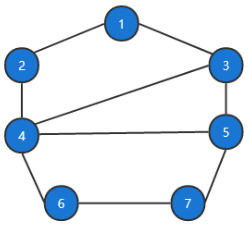
Above all, we introduce some knowledge about graph theory. Let $\mathcal{G}=\left(\mathcal{V},\mathcal{E}\right)$ represent an undirected network composed of n agents, where $\mathcal{V}$ denotes the set of agents and $\mathcal{E}$ denotes the set of edges. The neighborhood of the i-th agent is recorded as ${\mathcal{N}}_i=\left\{j\left|\left(i,j\right)\in \mathcal{E}\right.\right\}$. Specifically, when there is at least one path in any two agents in an undirected network $\mathcal{G}$, the network is connected.

Let ${\mathbb{R}}^n$ denote the n-dimensional Euclidean space and $∥·∥$ denote the Euclidean norm of a vector $x\in {\mathbb{R}}^n$. The notation ${\rho }_{max}\left(·\right)$ is the spectral radius of a matrix, and $\mathbb{N}$ represents the set of positive integers. Then let ${\mathrm{X}}_0\left({\mathbb{R}}^n\right)$ denote the collection of all proper lower semi-continuous convex functions from ${\mathbb{R}}^n$ to $\left(-\infty ,+\infty \right]$. When $W_i$ denotes a positive definite matrix, using $W_i$ as the diagonal element can form a positive definite diagonal matrix $\mathrm{blkdiag}{\left\{W_i\right\}}_{i\in \mathcal{V}}$. Let $\mathrm{ri}\left(·\right)$ denote the interior of a convex subset and $\mathrm{do}{\mathrm{m}}_f$ denote the effective domain of f. The subdifferential of function $f_i$ is expressed as $\partial f\left(x_1\right)=\{v\in {\mathbb{R}}^n|{\left(x_2-x_1\right)}^{\mathrm{T}}v\le f\left(x_2\right)-f\left(x_1\right),\forall x_2\in {\mathbb{R}}^n\}.$ The proximity operator of a function $f\in {\mathrm{X}}_0\left({\mathbb{R}}^n\right)$ related to ${\parallel ·\parallel }_P$ is defined by $pro{x}_{P^{-1}f}\left(x\right)=arg{min}_{y\in {\mathbb{R}}^n}\{f\left(y\right)+(1/2)\left|\right|x-y{\left|\right|}_P^2\}.$ The convex conjugate function of f is written as $f^{\otimes }$.

At the same time, we give the following lemmas and assumptions.

Lemma 1

([24]). Let $f\in {\mathrm{X}}_0\left({\mathbb{R}}^n\right)$, then for vectors $x_1,x_2\in {\mathbb{R}}^n$, the following relation holds:

$$\begin{array}{cc}\hfill x_2\in \partial f\left(x_1\right)\iff x_1& =pro{x}_f\left(x_1+x_2\right)\hfill \\ \hfill \iff x_2& =\left(I-pro{x}_f\right)\left(x_1+x_2\right).\hfill \end{array}$$

(3)

Lemma 2

([25]). Let $f\in {\mathrm{X}}_0\left({\mathbb{R}}^n\right)$, then both $pro{x}_f$ and $I-pro{x}_f$ satisfy a firmly nonexpansive relationship.

Lemma 3

([19]). For a fixed point iteration $u_{k+1}=T\left(u_k\right)$, $\left\{u_k\right\}$ will converge to the fixed point of T when it satisfies the following conditions:

1.

T is continuous,

2.

$\left\{\left|\right|u_k-u^{*}|{|}^2\right\}$ is non-increasing,

3.

$\underset{k\to \infty }{lim}{∥u_{k+1}-u_k∥}^2=0.$

Definition 1.

For all $x_1,x_2\in {\mathbb{R}}^n$, if an operator T satisfies $∥T{x}_1-T{x}_2∥\le ∥x_1-x_2∥$, then T is a nonexpansive operator. Further, if T satisfies ${∥T{x}_1-T{x}_2∥}^2\le {\left(T{x}_1-T{x}_2\right)}^{\mathrm{T}}\left(x_1-x_2\right)$, then T is firmly a nonexpansive operator.

Definition 2.

When ${\left(T{x}_1-T{x}_2\right)}^{\mathrm{T}}\left(x_1-x_2\right)\ge {\sigma }_T{∥x_1-x_2∥}^2,x_1,x_2\in {\mathbb{R}}^n$ exist for a constant ${\sigma }_T>0$ and operator T, then operator T satisfies ${\sigma }_T$-strongly monotone.

The following assumptions will also be used.

Assumption 1.

Graph $\mathcal{G}$ satisfies undirected and connected operators.

Assumption 2.

The following three points are satisfied:

1. 

$f_i:{\mathbb{R}}^n\to \mathbb{R}$ is a smooth convex function, let $1/{\beta }_i$ be Lipschitz constant, then $f_i$ satisfies

$$\begin{array}{c}\hfill {\beta }_i∥\nabla f_i\left(x_1\right)-\nabla f_i\left(x_2\right)∥\le ∥x_1-x_2∥,\forall x_1,x_2\in {\mathbb{R}}^n,\end{array}$$

2. 

$g_i:{\mathbb{R}}^n\to \mathbb{R}$ is a convex non-smooth function,

3. 

Problem (2) has at least one solution.

3. Algorithm Development

In this section, we design and derive the synchronous algorithm and asynchronous algorithm.

We next carry on the equivalent transformation to problem (2) to facilitate the subsequent algorithm design. The constraint, $x_i=x_j$ in (2) can be written as the edge-based form

$$\begin{array}{c}\hfill E_{ij}{x}_i+E_{ji}{x}_j=0,\end{array}$$

(4)

where $E_{ij}=I\in {\mathbb{R}}^{n\times n}$ for $i<j$, and $E_{ij}=-I\in {\mathbb{R}}^{n\times n}$ otherwise. Then, define the following linear operator:

$$\begin{array}{c}\hfill M_{(i,j)}:x\to (E_{ij}{x}_i,E_{ji}{x}_j)\in {\mathbb{R}}^{2n\times mn},\end{array}$$

(5)

with the compact variable $x={[x_1^{\mathrm{T}},\cdots ,x_m^{\mathrm{T}}]}^{\mathrm{T}}\in {\mathbb{R}}^{mn}$. We stack all $M_{(i,j)}$ to get the following operator:

$$\begin{array}{c}\hfill M:x\to {\left(M_{\left(i,j\right)}x\right)}_{\left(i,j\right)\in \mathcal{E}},\end{array}$$

(6)

with the dimension $2n\left|\mathcal{E}\right|\times mn$, where $\left|\mathcal{E}\right|$ is the number of edges of the network $\mathcal{E}$. Considering the set

$$\begin{array}{c}\hfill C_{\left(i,j\right)}=\left\{\left(e_1,e_2\right)\in {\mathbb{R}}^n\times {\mathbb{R}}^n\left|e_1+e_2=0\right.\right\}.\end{array}$$

Then,  constraint (4) can be further reformulated in the following form:

$$\begin{array}{c}\hfill M_{(i,j)}x\in C_{(i,j)}.\end{array}$$

(7)

Based on the above analysis, problem (2) can be transformed into

$$\begin{array}{c}\hfill \begin{array}{c}\underset{x_i\in {\mathbb{R}}^n}{min}{\displaystyle \sum _{i=1}^m}{f}_i\left(x_i\right)+g_i\left(x_i\right)+{\displaystyle \sum _{i=1}^m}{\displaystyle \sum _{\left(i,j\right)\in \mathcal{E}}}{\delta }_{C_{\left(i,j\right)}}\left(M_{\left(i,j\right)}x\right),\hfill \end{array}\end{array}$$

(8)

where ${\delta }_C$ represents the indicator function, i.e., 

$$\begin{array}{c}\hfill {\delta }_{C_{\left(i,j\right)}}\left(M_{\left(i,j\right)}x\right)=\left\{\begin{array}{c}0,M_{\left(i,j\right)}x\in C_{\left(i,j\right)},\hfill \\ +\infty ,M_{\left(i,j\right)}x\notin C_{\left(i,j\right)}.\hfill \end{array}\right.\end{array}$$

Then, let

$$\begin{array}{cc}& f\left(x\right)=\sum _{i=1}^m{f}_i\left(x_i\right),\hfill \\ & g\left(x\right)=\sum _{i=1}^m{g}_i\left(x_i\right),\hfill \\ & {\delta }_C\left(Mx\right)=\sum _{i=1}^m\sum _{j\in {\mathcal{N}}_i}{\delta }_{C_{\left(i,j\right)}}\left(M_{\left(i,j\right)}x\right),\hfill \end{array}$$

and $C={\prod }_{(i,j)\in \mathcal{E}}{C}_{(i,j)}$ ($\prod$ denotes the Cartesian product). Hence, the compact form of problem (8) can be expressed by

$$\begin{array}{c}\hfill \underset{x\in {\mathbb{R}}^{mn}}{min}f\left(x\right)+g\left(x\right)+{\delta }_C\left(Mx\right).\end{array}$$

(9)

3.1. Synchronous Algorithm 1

According to the fixed point theory, we design the distributed optimization algorithm of problem (2) from (9). We define the step-size matrices $\mathrm{\Gamma }=\mathrm{blkdiag}{\left\{{\gamma }_i{I}_n\right\}}_{i\in \mathcal{V}}$, $\tilde{\mathrm{\Lambda }}=\mathrm{blkdiag}{\left\{{\tilde{\lambda }}_{\left(i,j\right)}{{\tilde{\gamma }}_{\left(i,j\right)}}^{-1}\right\}}_{\left(i,j\right)\in \mathcal{E}}$, and $\tilde{\mathrm{H}}=\mathrm{blkdiag}{\left\{{\lambda }_{\left(i,j\right)}{I}_{2n}\right\}}_{\left(i,j\right)\in \mathcal{E}}$, where we let ${\tilde{\gamma }}_{\left(i,j\right)}=\mathrm{blkdiag}\left\{{\gamma }_i{I}_n,{\gamma }_j{I}_n\right\}$, and then introduce the following operators:

$$T_0\left(s^{*},x^{*}\right)=pro{x}_{\mathrm{\Gamma }g}\left(\begin{array}{c}{x}^{*}-\mathrm{\Gamma }\nabla f\left(x^{*}\right)-{\left(\tilde{\mathrm{H}}M\right)}^{\mathrm{T}}{s}^{*}\hfill \end{array}\right),$$

(10)

$${\tilde{T}}_1\left(s^{*},x^{*}\right)=\left(I-pro{x}_{{\tilde{\mathrm{\Lambda }}}^{-1}{\delta }_C}\right)\left(M{T}_0\left(s^{*},x^{*}\right)+s^{*}\right),$$

(11)

$$T_2\left(s^{*},x^{*}\right)=pro{x}_{\mathrm{\Gamma }g}\left(x^{*}-\mathrm{\Gamma }\nabla f\left(x^{*}\right)-{\left(\tilde{\mathrm{H}}M\right)}^{\mathrm{T}}{\tilde{T}}_1\left(s^{*},x^{*}\right)\right),$$

(12)

$$T\left(s^{*},x^{*}\right)=\left({\tilde{T}}_1\left(s^{*},x^{*}\right),T_2\left(s^{*},x^{*}\right)\right),$$

(13)

where $x^{*}=\mathrm{col}{\left\{x_i^{*}\right\}}_{i=1}^m$ and $s^{*}=\mathrm{col}{\left\{s_{\left(i,j\right)}^{*}\right\}}_{\left(i,j\right)\in \mathcal{E}}$ with $s_{\left(i,j\right)}^{*}=\mathrm{col}\{s_{\left(i,j\right),i}^{*},s_{\left(i,j\right),i}^{*}\}$ are the fixed points of T. In particular, $s_{\left(i,j\right),i}^{*}$ and $s_{\left(i,j\right),j}^{*}$ are maintained by i and j, respectively. Considering the update variables $y_{k+1}=\mathrm{col}{\left\{y_i^{k+1}\right\}}_{i=1}^m$, $x_{k+1}=\mathrm{col}{\left\{x_i^{k+1}\right\}}_{i=1}^m$, and $s_{k+1}=\mathrm{col}{\left\{s_{\left(i,j\right)}^{k+1}\right\}}_{\left(i,j\right)\in \mathcal{E}}$ with the edge-based variable $s_{\left(i,j\right)}^{k+1}=\mathrm{col}\{s_{\left(i,j\right),i}^{k+1},s_{\left(i,j\right),j}^{k+1}\}$, we give the Picard sequence of T and obtain the following update rules:

$$\begin{array}{c}\hfill \begin{array}{c}{y}_{k+1}=pro{x}_{\mathrm{\Gamma }g}\left(x_k-\mathrm{\Gamma }\nabla f\left(x_k\right)-{\left(\tilde{H}M\right)}^{\mathrm{T}}{s}_k\right)\hfill \\ s_{k+1}=\left(I-pro{x}_{{\tilde{\mathrm{\Lambda }}}^{-1}{\delta }_C}\right)\left(M{y}_{k+1}+s_k\right)\hfill \\ x_{k+1}=pro{x}_{\mathrm{\Gamma }g}\left(x_k-\mathrm{\Gamma }\nabla f\left(x_k\right)-{\left(\tilde{H}M\right)}^{\mathrm{T}}{s}_{k+1}\right)\hfill \end{array}\end{array}$$

(14)

Let ${\overline{w}}_{k+1}=\mathrm{col}{\left\{{\overline{w}}_{\left(i,j\right)}^{k+1}\right\}}_{\left(i,j\right)\in \mathcal{E}}=\mathrm{col}{\{{\tilde{\lambda }}_{\left(i,j\right)}{\tilde{\gamma }}_{\left(i,j\right)}^{-1}·s_{\left(i,j\right)}^{k+1}\}}_{\left(i,j\right)\in \mathcal{E}}$. Using Lemma 2, (14) can be rewritten as

$$y_{k+1}=pro{x}_{\mathrm{\Gamma }g}\left(x_k-\mathrm{\Gamma }\nabla f\left(x_k\right)-\mathrm{\Gamma }{M}^{\mathrm{T}}{\tilde{w}}_k\right),$$

(15a)

$$s_{k+1}=\left(I-pro{x}_{{\tilde{\mathrm{\Lambda }}}^{-1}{\delta }_C}\right)\left(M{y}_{k+1}+s_k\right),$$

(15b)

$$x_{k+1}=pro{x}_{\mathrm{\Gamma }g}\left(x_k-\mathrm{\Gamma }\nabla f\left(x_k\right)-\mathrm{\Gamma }{M}^{\mathrm{T}}{\tilde{w}}_{k+1}\right).$$

(15c)

Next, we split (15a)–(15c) in a distributed manner. It follows from (5) and (6) that the i-th component of $M^{\mathrm{T}}{\tilde{w}}_{k+1}$ is $E_{ij}{\tilde{w}}_{\left(i,j\right),i}^{k+1}$. Note that (15a) can be decomposed into

$$\begin{array}{c}\hfill \left(\begin{array}{c}{y}_1^{k+1}\\ ⋮\\ y_m^{k+1}\end{array}\right)=\left(\begin{array}{c}pro{x}_{{\gamma }_1{g}_1}\left(x_1^k-{\gamma }_1\nabla f_1\left(x_1^k\right)-{\gamma }_1{\sum }_{j\in {\mathcal{N}}_1}{E}_{1j}{\tilde{w}}_{\left(1,j\right),1}^k\right)\\ ⋮\\ pro{x}_{{\gamma }_m{g}_m}\left(x_m^k-{\gamma }_m\nabla f_m\left(x_m^k\right)-{\gamma }_m{\sum }_{j\in {\mathcal{N}}_m}{E}_{mj}{\tilde{w}}_{\left(m,j\right),m}^k\right)\end{array}\right).\end{array}$$

(16)

For (15b), multiply both sides of the equality by $\tilde{\mathrm{\Lambda }}$. As done in (16), we also split (15b) and (15c) and use the result $pro{x}_{{\delta }_{C_{(}i,j)}}=pro{j}_{C_{(}i,j)}$ to get the semi-distributed form:

$$y_i^{k+1}=pro{x}_{{\gamma }_i{g}_i}\left(\begin{array}{c}{x}_i^k-{\gamma }_i\nabla f_i\left(x_i^k\right)-{\gamma }_i\sum _{j\in {\mathcal{N}}_i}{E}_{ij}{\tilde{w}}_{\left(i,j\right),i}^k\hfill \end{array}\right),$$

(17a)

$${\tilde{w}}_{\left(i,j\right)}^{k+1}={\tilde{w}}_{\left(i,j\right)}^k+{\tilde{\lambda }}_{\left(i,j\right)}{\tilde{\gamma }}_{\left(i,j\right)}^{-1}\left(\begin{array}{c}{M}_{\left(i,j\right)}{y}^{k+1}-pro{j}_{C_{\left(i,j\right)}}\left(\begin{array}{c}\frac{{\tilde{\gamma }}_{\left(i,j\right)}}{{\tilde{\lambda }}_{\left(i,j\right)}}{\tilde{w}}_{\left(i,j\right)}^k+M_{\left(i,j\right)}{y}^{k+1}\hfill \end{array}\right)\hfill \end{array}\right),$$

(17b)

$$x_i^{k+1}=pro{x}_{{\gamma }_i{g}_i}\left(\begin{array}{c}{x}_i^k-{\gamma }_i\nabla f_i\left(x_i^k\right)-{\gamma }_i\sum _{j\in {\mathcal{N}}_i}{E}_{ij}{\tilde{w}}_{\left(i,j\right),i}^{k+1}\hfill \end{array}\right).$$

(17c)

Note that (17b) is not fully distributed due to the structure $w_{\left(i,j\right)}^{k+1}=\mathrm{col}\{w_{\left(i,j\right),i}^{k+1},w_{\left(i,j\right),j}^{k+1}\}$. By using (4) and (5), we can derive that the projection of vectors $e_1,e_2\in {\mathbb{R}}^n$ to $C_{\left(i,j\right)}$ is expressed as

$$\begin{array}{c}\hfill pro{j}_{C_{\left(i,j\right)}}\left(e_1,e_2\right)=\frac{1}{2}\left(e_1-e_2,e_2-e_1\right),\end{array}$$

which contributes to the local update of (17b), i.e.,

$$\begin{array}{cc}& {\tilde{w}}_{\left(i,j\right),i}^{k+1}={\tilde{w}}_{\left(i,j\right),i}^k+\frac{{\tilde{\lambda }}_{\left(i,j\right)}}{{\gamma }_i}\left(\begin{array}{c}{y}_i^{k+1}-\frac{1}{2}\left(\begin{array}{c}\left(\frac{{\gamma }_i}{{\tilde{\lambda }}_{\left(i,j\right)}}{\tilde{w}}_{\left(i,j\right),i}^k+y_i^{k+1}\right)-\left(\begin{array}{c}\frac{{\gamma }_i}{{\tilde{\lambda }}_{\left(i,j\right)}}{\tilde{w}}_{\left(i,j\right),j}^k-y_j^{k+1}\hfill \end{array}\right)\hfill \end{array}\right)\hfill \end{array}\right),\hfill \end{array}$$

$$\begin{array}{cc}& {\tilde{w}}_{\left(i,j\right),j}^{k+1}={\tilde{w}}_{\left(i,j\right),j}^k+\frac{{\tilde{\lambda }}_{\left(i,j\right)}}{{\gamma }_j}\left(\begin{array}{c}-y_j^{k+1}-\frac{1}{2}\left(\begin{array}{c}\left(\frac{{\gamma }_j}{{\tilde{\lambda }}_{\left(i,j\right)}}{\tilde{w}}_{\left(i,j\right),j}^k-y_j^{k+1}\right)-\left(\begin{array}{c}\frac{{\gamma }_j}{{\tilde{\lambda }}_{\left(i,j\right)}}{\tilde{w}}_{\left(i,j\right),i}^k+y_i^{k+1}\hfill \end{array}\right)\hfill \end{array}\right)\hfill \end{array}\right).\hfill \end{array}$$

Therefore, according to (17a), (17c), and the update of $w_{\left(i,j\right),i}^{k+1}$, we can summarize the synchronous distributed algorithm as follows:

Remark 1.

Notice that Algorithm 1 is completely distributed without involving any global parameters. For example, each agent individually maintains the private primal variable $x_i^k$, auxiliary variable $y_i^k$, and edge-based variables ${\tilde{w}}_{\left(i,j\right),i}^{k+1}$. For each edge $\left(i,j\right)\in \mathcal{E}$ in the network, ${\tilde{w}}_{\left(i,j\right)}^k=\mathrm{col}\{{\tilde{w}}_{\left(i,j\right),i}^k,{\tilde{w}}_{\left(i,j\right),i}^k\}$ as an auxiliary profile contains two components, i.e., ${\tilde{w}}_{\left(i,j\right),i}^k$ and ${\tilde{w}}_{\left(i,j\right),i}^k$, which are respectively kept by i and j. Meanwhile, the information exchange is locally conducted; that is, agent i shares its updated data $y_i^{k+1}$ and ${\tilde{w}}_{\left(i,j\right),i}^{k+1}$ with its all neighbors $j\in {\mathcal{N}}_i$. On the other hand, the proposed algorithm takes uncoordinated constant positive step-sizes, ${\gamma }_i$, essentially distinguished from the global and dynamic ones in [7,8,9,14,23]. It is also worth noting that the edge-based step-size ${\tilde{\lambda }}_{\left(i,j\right)}$, held by agents i and j linked by the edge $\left(i,j\right)\in \mathcal{E}$, can be seen as inherent parameters of the communication network, revealing the quality of the communication.

Algorithm 1 Distributed algorithm based on proximal operators

Input: For all agents $i\in \mathcal{V}$, $x_i^0\in {\mathbb{R}}^n$, and  ${\tilde{w}}_{\left(i,j\right),i}^0\in {\mathbb{R}}^n$, where $j\in {\mathcal{N}}_i$. And select proper positive step-sizes or parameters, ${\gamma }_i$ and ${\tilde{\lambda }}_{\left(i,j\right)}$. For $k=0,1,\dots ,\mathbf{do}$:  1. $y_i^{k+1}=pro{x}_{{\gamma }_i{g}_i}\left(\begin{array}{c}{x}_i^k-{\gamma }_i\nabla f_i\left(x_i^k\right)-{\gamma }_i{\sum }_{j\in {\mathcal{N}}_i}{E}_{ij}{\tilde{w}}_{\left(i,j\right),i}^k\hfill \end{array}\right),$  2. ${\tilde{w}}_{\left(i,j\right),i}^{k+1}=\frac{1}{2}\frac{{\tilde{\lambda }}_{\left(i,j\right)}}{{\gamma }_i}\left(y_i^{k+1}-y_j^{k+1}\right)$$+\frac{1}{2}\left({\tilde{w}}_{\left(i,j\right),i}^k+{\tilde{w}}_{\left(i,j\right),j}^k\right),\forall j\in {\mathcal{N}}_i,$  3. $x_i^{k+1}=pro{x}_{{\gamma }_i{g}_i}\left(\begin{array}{c}{x}_i^k-{\gamma }_i\nabla f_i\left(x_i^k\right)-{\gamma }_i{\sum }_{j\in {\mathcal{N}}_i}{E}_{ij}{\tilde{w}}_{\left(i,j\right),i}^{k+1}\hfill \end{array}\right),$  4. Send $y_i^{k+1}$, ${\tilde{w}}_{\left(i,j\right),i}^{k+1}$ to j for $j\in {\mathcal{N}}_i$,  5. Until the $∥x_i^{k+1}-x_i^k∥$ approaches zero. End Output: The primal variable $x_i^{k+1}$ as the optimal solution $x_i^{*}$.

3.2. Asynchronous Algorithm 2

Here, we extend the synchronous Algorithm 1 to the asynchronous iterative version based on the random-block coordinate mechanism in [2]. Combining with the principle of this mechanism, we define the diagonal matrix $P_i\in {\mathbb{R}}^{\left(2\left|\mathcal{E}\right|+m\right)n}\times {\mathbb{R}}^{\left(2\left|\mathcal{E}\right|+m\right)n}$ (where $\left|\mathcal{E}\right|$ denotes the number of edges of the graph $\mathcal{E}$) diagonal elements of 0 or 1 to represent the coordinate matrix, and then divide the vector $\left(s,x\right)$ into m blocks. At the same time, we define the activation vector ${\xi }^k\in {\mathbb{R}}^m$ of $\varphi$-valued, where $\varphi =0,1$ is a binary string with length m. When ${\xi }_i^k=1$, it means that the agent i is activated at the k-th iteration; otherwise it is not activated.

In order to describe the activation state of different coordinate blocks and ensure random activation, we give the following assumption.

Assumption 3.

The following two points are satisfied:

1.

The sum of $P{}_i$ satisfies ${\sum }_i^m{P}_i=I$,

2.

${\left({\xi }^k\right)}_{k\ge 0}$ is a ϕ-valued vector satisfying identical independent distributionsand its probability is $p_i=\mathbb{P}\left({\xi }_i^k=1\right)>0,k\ge 0.$

Then, based on the given assumption, we can develop the asynchronous algorithm as follows:

It can be seen that Algorithm 2 allows each agent to awaken with an independent probability, which means that a subset of randomly activated agents will participate in the updates while inactivated ones stay in previous states. Such a scheme is more flexible than the single waking-up scheme [22] or other activated block coordinates that are uniformly selected [26]. In addition, the probability is completely independent of the others, which does not meet some strict conditions, such as ${\sum }_{i=1}^m{p}_i=1$.

Algorithm 2 Asynchronous distributed version

Input: For all agents $i\in \mathcal{V}$, $x_i^0\in {\mathbb{R}}^{n_i}$, and ${\tilde{w}}_{\left(i,j\right),i}^0\in {\mathbb{R}}^n$, where $j\in {\mathcal{N}}_i$. And select proper positive step-sizes or parameters, ${\gamma }_i$ and ${\tilde{\lambda }}_{\left(i,j\right)}$. For $k=0,1,\dots ,\mathbf{do}:$ For $j\in {\mathcal{N}}_i$, each agent i is activated independently with probability $p_i$, and further performs the update steps 1–5 in Algorithm 1. While agents that are not activated, the last values keep unchanged. End Output: The primal variable $x_i^{k+1}$ as the optimal solution $x_i^{*}$.

In order to facilitate the subsequent derivation of convergence, we need to give a compact form of Algorithm 2. By making $u=(s,x)$, we get

$$\begin{array}{c}\hfill u_{k+1}=u_k+E_{k+1}\left(T{u}_k-u_k\right),\end{array}$$

(18)

where $E_{k+1}={\sum }_{i=1}^m{\xi }_i^{k+1}{P}_i$ and operator T can be seen in Equation (11).

4. Convergence Analysis

The convergence proof of the algorithms is provided in this section. The following assumption is the condition to be met for the convergence of the algorithms.

Assumption 4.

Recall the local Lipschitz constant ${\beta }_i$ in Assumption 2. It is assumed that the step-sizes satisfy the following conditions:

$$\begin{array}{c}\hfill 0<{\gamma }_i<2{\beta }_i,0<{\tilde{\lambda }}_{\left(i,j\right)}<1.\end{array}$$

Lemma 4.

Let $x^{*}$ be a solution to (9), then there are

$$\begin{array}{cc}& s^{*}={\tilde{T}}_1\left(s^{*},x^{*}\right),\hfill \\ & x^{*}=T_2\left(s^{*},x^{*}\right),\hfill \end{array}$$

which means $u^{*}=\left(s^{*},x^{*}\right)$ is a fixed point of T. On the contrary, $x^{*}$ is the solution to (9) when $u^{*}$ is the fixed point of T.

Proof. 

Use the first-order optimal condition of (9) to obtain $0\in \mathrm{\Gamma }\nabla f\left(x^{*}\right)+\mathrm{\Gamma }\partial g\left(x^{*}\right)+\mathrm{\Gamma }{M}^{\mathrm{T}}\partial {\delta }_C\left(M{x}^{*}\right)$, where $x^{*}$ is the optimal solution. According to the definition of matrix step-sizes, we further obtain

$$\begin{array}{cc}\hfill 0\in & \mathrm{\Gamma }\nabla f\left(x^{*}\right)+\mathrm{\Gamma }\partial g\left(x^{*}\right)+{\left(\tilde{\mathrm{H}}M\right)}^{\mathrm{T}}{\tilde{\mathrm{\Lambda }}}^{-1}\partial {\delta }_C\left(M{x}^{*}\right).\hfill \end{array}$$

Use Lemma 1 and let $s^{*}\in {\tilde{\mathrm{\Lambda }}}^{-1}\partial {\delta }_C\left(M{x}^{*}\right)$ to get

$$\begin{array}{c}\hfill s^{*}=\left(I-pro{x}_{{\tilde{\mathrm{\Lambda }}}^{-1}{\delta }_C}\right)\left(M{x}^{*}+s^{*}\right),\end{array}$$

(19)

$$\begin{array}{c}\hfill x^{*}=pro{x}_{\mathrm{\Gamma }g}\left(x^{*}-\mathrm{\Gamma }\nabla f\left(x^{*}\right)-{\left(\tilde{\mathrm{H}}M\right)}^{\mathrm{T}}{s}^{*}\right).\end{array}$$

(20)

Then according to (19) and (20), we can get

$$\begin{array}{c}\hfill s^{*}=\left(I-pro{x}_{{\tilde{\mathrm{\Lambda }}}^{-1}{\delta }_C}\right)\left(Mpro{x}_{\mathrm{\Gamma }g}\left(\begin{array}{c}{x}^{*}-\mathrm{\Gamma }\nabla f\left(x^{*}\right)-{\left(\tilde{\mathrm{H}}M\right)}^{\mathrm{T}}{s}^{*}\hfill \end{array}\right)+s^{*}\right).\end{array}$$

Therefore, we have $x^{*}=T_2\left(s^{*},x^{*}\right)$ and $s^{*}={\tilde{T}}_1\left(s^{*},x^{*}\right)$. Meanwhile, $u^{*}=T{u}^{*}$, where $u^{*}=\left(s^{*},x^{*}\right)$. Accordingly, if there is $u^{*}=T{u}^{*}$, it can also be deduced that $x^{*}$ satisfies the first-order optimality condition of problem (9). Thus $x^{*}$ is an optimal solution of problem (9). □

Lemma 5.

Let Assumptions 1 and 2 hold, then there are

$$\begin{array}{c}\hfill {∥s_{k+1}-s^{*}∥}_{\tilde{\mathrm{\Lambda }}}^2\le {∥s_k-s^{*}∥}_{\tilde{\mathrm{\Lambda }}}^2-{∥s_{k+1}-s_k∥}_{\tilde{\mathrm{\Lambda }}}^2+2{\left(s_{k+1}-s^{*}\right)}^{\mathrm{T}}\tilde{\mathrm{\Lambda }}M\left(y_{k+1}-x^{*}\right),\end{array}$$

(21)

$$\begin{array}{cc}& {∥x_{k+1}-x^{*}∥}_{{\mathrm{\Gamma }}^{-1}}^2\hfill \\ & \le {∥x_k-x^{*}∥}_{{\mathrm{\Gamma }}^{-1}}^2-{∥x_{k+1}-y_{k+1}∥}_{{\mathrm{\Gamma }}^{-1}}^2-{∥x_k-y_{k+1}∥}_{{\mathrm{\Gamma }}^{-1}}^2\hfill \\ & +2{\left({\mathrm{\Gamma }}^{-1}{x}_{k+1}-{\mathrm{\Gamma }}^{-1}{y}_{k+1}\right)}^{\mathrm{T}}\left(\begin{array}{c}\mathrm{\Gamma }\nabla f\left(x_k\right)+{\left(\tilde{\mathrm{H}}M\right)}^{\mathrm{T}}{s}_k\hfill \end{array}\right)\hfill \\ & +2{\left({\mathrm{\Gamma }}^{-1}{x}^{*}-{\mathrm{\Gamma }}^{-1}{x}_{k+1}\right)}^{\mathrm{T}}\left(\begin{array}{c}\mathrm{\Gamma }\nabla f\left(x_k\right)+{\left(\tilde{\mathrm{H}}M\right)}^{\mathrm{T}}{s}_{k+1}\hfill \end{array}\right)\hfill \\ & +2\left((g\circ \mathrm{\Gamma })\left({\mathrm{\Gamma }}^{-1}{x}^{*}\right)-\left(g\circ \mathrm{\Gamma }\right)\left({\mathrm{\Gamma }}^{-1}{y}_{k+1}\right)\right).\hfill \end{array}$$

(22)

Proof. 

Combining (14), (19), and Lemma 2, we get

$$\begin{array}{cc}& {∥s_{k+1}-s^{*}∥}_{\tilde{\mathrm{\Lambda }}}^2\hfill \\ & ={∥\begin{array}{c}\left(I-pro{x}_{{\tilde{\mathrm{\Lambda }}}^{-1}{\delta }_C}\right)\left(M{y}_{k+1}+s_k\right)-\left(I-pro{x}_{{\tilde{\mathrm{\Lambda }}}^{-1}{\delta }_C}\right)\left(M{x}^{*}+s^{*}\right)\hfill \end{array}∥}_{\tilde{\mathrm{\Lambda }}}^2\hfill \end{array}$$

$$\begin{array}{c}\hfill \le {\left(s_{k+1}-s^{*}\right)}^{\mathrm{T}}\tilde{\mathrm{\Lambda }}\left(\left(M{y}_{k+1}+s_k\right)-\left(M{x}^{*}+s^{*}\right)\right).\end{array}$$

It is further concluded that

$$\begin{array}{cc}& {\left(s_{k+1}-s^{*}\right)}^{\mathrm{T}}\tilde{\mathrm{\Lambda }}\left(s_{k+1}-s_k+s_k-s^{*}\right)\hfill \\ & \le {\left(s_{k+1}-s^{*}\right)}^{\mathrm{T}}\tilde{\mathrm{\Lambda }}M\left(y_{k+1}-x^{*}\right)+{\left(s_{k+1}-s^{*}\right)}^{\mathrm{T}}\tilde{\mathrm{\Lambda }}\left(s_k-s^{*}\right).\hfill \end{array}$$

Here we introduce an equality. For a positive definite matrix $\mathrm{K}$ and $x_1,x_2,x_3\in {\mathbb{R}}^n$, we have

$$\begin{array}{c}\hfill 2{\left(x_1-x_2\right)}^{\mathrm{T}}\mathrm{K}\left(x_3-x_2\right)={∥x_3-x_2∥}_{\mathrm{K}}^2+{∥x_1-x_2∥}_{\mathrm{K}}^2-{∥x_1-x_3∥}_{\mathrm{K}}^2.\end{array}$$

(23)

Combining the above two results, we derive

$$\begin{array}{cc}\hfill {∥s_{k+1}-s^{*}∥}_{\tilde{\mathrm{\Lambda }}}^2=& {∥s_k-s^{*}∥}_{\tilde{\mathrm{\Lambda }}}^2-{∥s_{k+1}-s_k∥}_{\tilde{\mathrm{\Lambda }}}^2+2{\left(s_{k+1}-s^{*}\right)}^{\mathrm{T}}\tilde{\mathrm{\Lambda }}\left(s_{k+1}-s_k\right)\hfill \\ \hfill \le & {∥s_k-s^{*}∥}_{\tilde{\mathrm{\Lambda }}}^2-{∥s_{k+1}-s_k∥}_{\tilde{\mathrm{H}}}^2+2{\left(s_{k+1}-s^{*}\right)}^{\mathrm{T}}\tilde{\mathrm{\Lambda }}M\left(y_{k+1}-x^{*}\right).\hfill \end{array}$$

(24)

In order to prove the validity of (22), (3) is used for (14)

$$\begin{array}{c}\hfill {\mathrm{\Gamma }}^{-1}\left(x_k-\mathrm{\Gamma }\nabla f\left(x_k\right)-{\left(\tilde{\mathrm{H}}M\right)}^{\mathrm{T}}{s}_{k+1}-x_{k+1}\right)\in \partial g\left(x_{k+1}\right).\end{array}$$

Using subdifferential properties to obtain

$$\begin{array}{c}\hfill {\left(x^{*}-x_{k+1}\right)}^{\mathrm{T}}{\mathrm{\Gamma }}^{-1}\left(x_k-\mathrm{\Gamma }\nabla f\left(x_k\right)-{\left(\tilde{\mathrm{H}}M\right)}^{\mathrm{T}}{s}_{k+1}-x_{k+1}\right)\le g\left(x^{*}\right)-g\left(x_{k+1}\right)\end{array}$$

and equivalent

$$\begin{array}{cc}\hfill & {\left({\mathrm{\Gamma }}^{-1}{x}_{k+1}-{\mathrm{\Gamma }}^{-1}{x}^{*}\right)}^{\mathrm{T}}\left(x_{k+1}-x_k\right)\hfill \\ \hfill & \le -{\left({\mathrm{\Gamma }}^{-1}{x}_{k+1}-{\mathrm{\Gamma }}^{-1}{x}^{*}\right)}^{\mathrm{T}}{\mathrm{\Gamma }}^{-1}\left(\begin{array}{c}\mathrm{\Gamma }\nabla f\left(x_k\right)+{\left(\tilde{\mathrm{H}}M\right)}^{\mathrm{T}}{s}_{k+1}\hfill \end{array}\right)\hfill \\ \hfill & +\left(g\circ \mathrm{\Gamma }\right)\left({\mathrm{\Gamma }}^{-1}{x}^{*}\right)-\left(g\circ \mathrm{\Gamma }\right)\left({\mathrm{\Gamma }}^{-1}{x}_{k+1}\right).\hfill \end{array}$$

(25)

Moreover, there is

$$\begin{array}{cc}\hfill {∥x_{k+1}-x^{*}∥}_{{\mathrm{\Gamma }}^{-1}}^2=& {∥x_k-x^{*}∥}_{{\mathrm{\Gamma }}^{-1}}^2-{∥x_{k+1}-x_k∥}_{{\mathrm{\Gamma }}^{-1}}^2+2{\left(x_{k+1}-x^{*}\right)}^{\mathrm{T}}{\mathrm{\Gamma }}^{-1}\left(x_{k+1}-x_k\right).\hfill \end{array}$$

(26)

A derivation similar to (25) is obtained for (14)

$$\begin{array}{cc}\hfill & {\left({\mathrm{\Gamma }}^{-1}{x}_{k+1}-{\mathrm{\Gamma }}^{-1}{y}_{k+1}\right)}^{\mathrm{T}}\left(\begin{array}{c}{x}_k-\mathrm{\Gamma }\nabla f\left(x_k\right)-{\left(\tilde{\mathrm{H}}M\right)}^{\mathrm{T}}{s}_k-y_{k+1}\hfill \end{array}\right)\hfill \\ \hfill & \le \left(g\circ \mathrm{\Gamma }\right)\left({\mathrm{\Gamma }}^{-1}{x}_{k+1}\right)-\left(g\circ \mathrm{\Gamma }\right)\left({\mathrm{\Gamma }}^{-1}{y}_{k+1}\right)\hfill \\ \hfill & \iff {\left({\mathrm{\Gamma }}^{-1}{x}_{k+1}-{\mathrm{\Gamma }}^{-1}{y}_{k+1}\right)}^{\mathrm{T}}\left(x_k-y_{k+1}\right)\hfill \\ \hfill & \le {\left({\mathrm{\Gamma }}^{-1}{x}_{k+1}-{\mathrm{\Gamma }}^{-1}{y}_{k+1}\right)}^{\mathrm{T}}\left(\begin{array}{c}\mathrm{\Gamma }\nabla f\left(x_k\right)+{\left(\tilde{\mathrm{H}}M\right)}^{\mathrm{T}}{s}_k\hfill \end{array}\right)\hfill \\ \hfill & +\left(g\circ \mathrm{\Gamma }\right)\left({\mathrm{\Gamma }}^{-1}{x}_{k+1}\right)-\left(g\circ \mathrm{\Gamma }\right)\left({\mathrm{\Gamma }}^{-1}{y}_{k+1}\right).\hfill \end{array}$$

Therefore, we deduce

$$\begin{array}{cc}& -{∥x_{k+1}-x_k∥}_{{\mathrm{\Gamma }}^{-1}}^2\hfill \\ & =-{∥x_k-y_{k+1}∥}_{{\mathrm{\Gamma }}^{-1}}^2-{∥x_{k+1}-y_{k+1}∥}_{{\mathrm{\Gamma }}^{-1}}^2+2{\left(x_k-y_{k+1}\right)}^{\mathrm{T}}{\mathrm{\Gamma }}^{-1}\left(x_{k+1}-y_{k+1}\right)\hfill \end{array}$$

$$\begin{array}{cc}& \le -{∥x_k-y_{k+1}∥}_{{\mathrm{\Gamma }}^{-1}}^2-{∥x_{k+1}-y_{k+1}∥}_{{\mathrm{\Gamma }}^{-1}}^2\hfill \\ & +2{\left({\mathrm{\Gamma }}^{-1}{x}_{k+1}-{\mathrm{\Gamma }}^{-1}{y}_{k+1}\right)}^{\mathrm{T}}\left(\begin{array}{c}\mathrm{\Gamma }\nabla f\left(x_k\right)+{\left(\tilde{\mathrm{H}}M\right)}^{\mathrm{T}}{s}_k\hfill \end{array}\right)\hfill \\ & +2\left(\left(g\circ \mathrm{\Gamma }\right)\left({\mathrm{\Gamma }}^{-1}{x}_{k+1}\right)-\left(g\circ \mathrm{\Gamma }\right)\left({\mathrm{\Gamma }}^{-1}{y}_{k+1}\right)\right).\hfill \end{array}$$

Combining the above two equalities and (26), we can get (22). □

Lemma 6.

Let Assumptions 1 and 2 hold. Set $\mathbf{\beta }=\mathrm{blkdiag}{\left\{{\beta }_i{I}_n\right\}}_{i\in \mathcal{V}}$. For matrix $P=\mathrm{blkdiag}\{\tilde{\mathrm{\Lambda }},{\mathrm{\Gamma }}^{-1}\}$ and $u=\left(s,x\right)$, there is

$$\begin{array}{cc}\hfill & {∥u_{k+1}-u^{*}∥}_P^2\hfill \\ & \le {∥u_{k+1}-u^{*}∥}_P^2-{∥s_{k+1}-s_k∥}_{\tilde{\mathrm{\Lambda }}\left(I-M\mathrm{\Gamma }{M}^{\mathrm{T}}\tilde{\mathrm{\Lambda }}\right)}^2\hfill \\ & -{∥\begin{array}{c}{y}_{k+1}-x_{k+1}+{\left(\tilde{\mathrm{H}}M\right)}^{\mathrm{T}}\left(s_{k+1}-s_k\right)\hfill \end{array}∥}_{{\mathrm{\Gamma }}^{-1}}^2\hfill \\ & -{∥x_k-y_{k+1}-\left(\mathrm{\Gamma }\nabla f\left(x_k\right)-\mathrm{\Gamma }\nabla f\left(x^{*}\right)\right)∥}_{{\mathrm{\Gamma }}^{-1}}^2\hfill \\ & -{∥\nabla f\left(x_k\right)-\nabla f\left(x^{*}\right)∥}_{2\beta -\mathrm{\Gamma }}^2.\hfill \end{array}$$

(27)

Proof. 

Adding (21) and (22), then rearranging to get

$$\begin{array}{cc}& {∥x_{k+1}-x^{*}∥}_{{\mathrm{\Gamma }}^{-1}}^2+{∥s_{k+1}-s^{*}∥}_{\tilde{\mathrm{\Lambda }}}^2\hfill \\ & \le {∥x_k-x^{*}∥}_{{\mathrm{\Gamma }}^{-1}}^2+{∥s_k-s^{*}∥}_{\tilde{\mathrm{\Lambda }}}^2-{∥x_k-y_{k+1}∥}_{{\mathrm{\Gamma }}^{-1}}^2\hfill \\ & -{∥s_{k+1}-s_k∥}_{\tilde{\mathrm{\Lambda }}}^2-{∥x_{k+1}-y_{k+1}∥}_{{\mathrm{\Gamma }}^{-1}}^2\hfill \\ & +2{\left(\begin{array}{c}{\left(\tilde{\mathrm{H}}M\right)}^{\mathrm{T}}\left(s_{k+1}-s_k\right)\hfill \end{array}\right)}^{\mathrm{T}}{\mathrm{\Gamma }}^{-1}\left(y_{k+1}-x_{k+1}\right)\hfill \\ & +2{\left(\mathrm{\Gamma }\nabla f\left(x_k\right)-\mathrm{\Gamma }\nabla f\left(x^{*}\right)\right)}^{\mathrm{T}}{\mathrm{\Gamma }}^{-1}\left(x_k-y_{k+1}\right)\hfill \\ & -2{\left(\mathrm{\Gamma }\nabla f\left(x_k\right)-\mathrm{\Gamma }\nabla f\left(x^{*}\right)\right)}^{\mathrm{T}}{\mathrm{\Gamma }}^{-1}\left(x_k-x^{*}\right)\hfill \\ & +2\left(\begin{array}{c}{\left(\begin{array}{c}-\mathrm{\Gamma }\nabla f\left(x^{*}\right)-{\left(\tilde{\mathrm{H}}M\right)}^{\mathrm{T}}{s}^{*}\hfill \end{array}\right)}^{\mathrm{T}}{\mathrm{\Gamma }}^{-1}\left(y_{k+1}-x^{*}\right)\hfill \\ +(g\circ \mathrm{\Gamma })\left({\mathrm{\Gamma }}^{-1}{x}^{*}\right)-\left(g\circ \mathrm{\Gamma }\right)\left({\mathrm{\Gamma }}^{-1}{y}_{k+1}\right)\hfill \end{array}\right).\hfill \end{array}$$

Further, we have

$$\begin{array}{cc}\hfill & {∥x_{k+1}-x^{*}∥}_{{\mathrm{\Gamma }}^{-1}}^2+{∥s_{k+1}-s^{*}∥}_{\tilde{\mathrm{\Lambda }}}^2\hfill \\ & \le {∥x_k-x^{*}∥}_{{\mathrm{\Gamma }}^{-1}}^2+{∥s_k-s^{*}∥}_{\tilde{\mathrm{\Lambda }}}^2-{∥x_k-y_{k+1}∥}_{{\mathrm{\Gamma }}^{-1}}^2\hfill \\ & -{∥s_{k+1}-s_k∥}_{\tilde{\mathrm{\Lambda }}\left(I-M\mathrm{\Gamma }{M}^{\mathrm{T}}\tilde{\mathrm{\Lambda }}\right)}^2-{∥x_{k+1}-y_{k+1}∥}_{{\mathrm{\Gamma }}^{-1}}^2\hfill \\ & +{∥\begin{array}{c}{\left(\tilde{\mathrm{H}}M\right)}^{\mathrm{T}}\left(s_{k+1}-s_k\right)\hfill \end{array}∥}_{{\mathrm{\Gamma }}^{-1}}^2+{∥y_{k+1}-x_{k+1}∥}_{{\mathrm{\Gamma }}^{-1}}^2\hfill \\ & -{∥y_{k+1}-x_{k+1}+{\left(\tilde{\mathrm{H}}M\right)}^{\mathrm{T}}\left(s_{k+1}-s_k\right)∥}_{{\mathrm{\Gamma }}^{-1}}^2\hfill \\ & +{∥\mathrm{\Gamma }\nabla f\left(x_k\right)-\mathrm{\Gamma }\nabla f\left(x^{*}\right)∥}_{{\mathrm{\Gamma }}^{-1}}^2+{∥x_k-y_{k+1}∥}_{{\mathrm{\Gamma }}^{-1}}^2\hfill \\ & -{∥x_k-y_{k+1}-\left(\mathrm{\Gamma }\nabla f\left(x_k\right)-\mathrm{\Gamma }\nabla f\left(x^{*}\right)\right)∥}_{{\mathrm{\Gamma }}^{-1}}^2\hfill \\ & +2\left(\begin{array}{c}{\left(\begin{array}{c}-\mathrm{\Gamma }\nabla f\left(x^{*}\right)-{\left(\tilde{\mathrm{H}}M\right)}^{\mathrm{T}}{s}^{*}\hfill \end{array}\right)}^{\mathrm{T}}\left(y_{k+1}-x^{*}\right)\hfill \\ +(g\circ \mathrm{\Gamma })\left({\mathrm{\Gamma }}^{-1}{x}^{*}\right)-\left(g\circ \mathrm{\Gamma }\right)\left({\mathrm{\Gamma }}^{-1}{y}_{k+1}\right)\hfill \end{array}\right).\hfill \end{array}$$

(28)

Then we deal with some terms in the above inequality. For (20) combined with Lemma 1 can deduce

$$\begin{array}{cc}& -\mathrm{\Gamma }\nabla f\left(x^{*}\right)-{\left(\tilde{\mathrm{H}}M\right)}^{\mathrm{T}}{s}^{*}\in \mathrm{\Gamma }\partial g\left(x^{*}\right)=\partial \left(g\circ \mathrm{\Gamma }\right)\left({\mathrm{\Gamma }}^{-1}{x}^{*}\right).\hfill \end{array}$$

Further using subdifferential properties, we have

$$\begin{array}{c}{\left({\mathrm{\Gamma }}^{-1}{y}_{k+1}-{\mathrm{\Gamma }}^{-1}{x}^{*}\right)}^{\mathrm{T}}\left(\begin{array}{c}-\mathrm{\Gamma }\nabla f\left(x^{*}\right)-{\left(\tilde{\mathrm{H}}M\right)}^{\mathrm{T}}{s}^{*}\hfill \end{array}\right)\hfill \\ +\left(g\circ \mathrm{\Gamma }\right)\left({\mathrm{\Gamma }}^{-1}{x}^{*}\right)-\left(g\circ \mathrm{\Gamma }\right)\left({\mathrm{\Gamma }}^{-1}{y}_{k+1}\right)\le 0.\hfill \end{array}$$

Meanwhile, because $\nabla f_i$ is $1/{\beta }_i$-strongly monotone, there is

$$\begin{array}{c}\hfill -{\left(\nabla f\left(x_k\right)-\nabla f\left(x^{*}\right)\right)}^{\mathrm{T}}\left(x_k-x^{*}\right)\le -{∥\nabla f\left(x_k\right)-\nabla f\left(x^{*}\right)∥}_{\mathbf{\beta }}^2.\end{array}$$

(29)

Bring the above results back to (28) and get (27). □

Lemma 7.

Under Assumptions 1–4, $\left\{\left|\right|u_k-u^{*}{\left|\right|}_P^2\right\}$ is non-increasing and ${lim}_{k\to \infty }{∥u_{k+1}-u_k∥}_P^2=0$.

Proof. 

If Assumption 4 holds, we can deduce that $\left\{\left|\right|u_k-u^{*}{\left|\right|}_P^2\right\}$ satisfies non-increasing operators.

Sum (27) over k from 0 to N to obtain

$$\begin{array}{cc}& {∥u_{N+1}-u^{*}∥}_P^2\hfill \\ & \le {∥u_0-u^{*}∥}_P^2-\sum _{k=0}^n{∥s_{k+1}-s_k∥}_{\tilde{\mathrm{\Lambda }}\left(I-M\mathrm{\Gamma }{M}^{\mathrm{T}}\tilde{\mathrm{\Lambda }}\right)}^2\hfill \\ & -\sum _{k=0}^n{∥\begin{array}{c}\left(x_{k+1}-y_{k+1}\right)+{\left(\tilde{\mathrm{H}}M\mathrm{\Gamma }\right)}^{\mathrm{T}}\left(s_{k+1}-s_k\right)\hfill \end{array}∥}_{{\mathrm{\Gamma }}^{-1}}^2\hfill \\ & -\sum _{k=0}^n{∥x_k-y_{k+1}-\left(\mathrm{\Gamma }\nabla f\left(x_k\right)-\mathrm{\Gamma }\nabla f\left(x^{*}\right)\right)∥}_{{\mathrm{\Gamma }}^{-1}}^2\hfill \\ & -\sum _{k=0}^n{∥\nabla f\left(x_k\right)-\nabla f\left(x^{*}\right)∥}_{2\mathbf{\beta }-\mathrm{\Gamma }}^2.\hfill \end{array}$$

When N tends to infinity, we can get

$$\begin{array}{c}\hfill \begin{array}{c}{\displaystyle \sum _{k=0}^{\infty }}{∥s_{k+1}-s_k∥}_{\tilde{\mathrm{\Lambda }}\left(I-M\mathrm{\Gamma }{M}^{\mathrm{T}}\tilde{\mathrm{\Lambda }}\right)}<\infty ,\hfill \\ {\displaystyle \sum _{k=0}^{\infty }}∥\begin{array}{c}\left(x_{k+1}-y_{k+1}\right)+{\left(\tilde{\mathrm{H}}M\mathrm{\Gamma }\right)}^{\mathrm{T}}\left(s_{k+1}-s_k\right)\hfill \end{array}∥<\infty ,\hfill \\ {\displaystyle \sum _{k=0}^{\infty }}∥x_k-y_{k+1}-\left(\mathrm{\Gamma }\nabla f\left(x_k\right)-\mathrm{\Gamma }\nabla f\left(x^{*}\right)\right)∥<\infty ,\hfill \\ {\displaystyle \sum _{k=0}^{\infty }}∥\nabla f\left(x_k\right)-\nabla f\left(x^{*}\right)∥<\infty .\hfill \end{array}\end{array}$$

This means

$$\underset{k\to \infty }{lim}{∥s_{k+1}-s_k∥}_{\tilde{\mathrm{\Lambda }}\left(I-M\mathrm{\Gamma }{M}^{\mathrm{T}}\tilde{\mathrm{\Lambda }}\right)}=0,$$

(30)

$$\underset{k\to \infty }{lim}∥\begin{array}{c}\left(x_{k+1}-y_{k+1}\right)+{\left(\tilde{\mathrm{H}}M\mathrm{\Gamma }\right)}^{\mathrm{T}}\left(s_{k+1}-s_k\right)\hfill \end{array}∥=0,$$

(31)

$$\underset{k\to \infty }{lim}∥x_k-y_{k+1}-\left(\mathrm{\Gamma }\nabla f\left(x_k\right)-\mathrm{\Gamma }\nabla f\left(x^{*}\right)\right)∥=0,$$

(32)

$$\underset{k\to \infty }{lim}∥\nabla f\left(x^{*}\right)-\nabla f\left(x_k\right)∥=0.$$

(33)

Next, according to (32) and (33), we obtain

$$\begin{array}{c}\hfill \underset{k\to \infty }{lim}∥x_k-y_{k+1}∥=0.\end{array}$$

(34)

Meanwhile, if Assumption 4 holds, $I-M\mathrm{\Gamma }{M}^{\mathrm{T}}\tilde{\mathrm{\Lambda }}$ is a symmetric positive definite. Therefore, we can get

$$\begin{array}{c}\hfill \underset{k\to \infty }{lim}∥s_{k+1}-s_k∥=0.\end{array}$$

(35)

According to (31) and (35) we obtain ${lim}_{k\to \infty }∥x_{k+1}-y_{k+1}∥=0.$ Combining with (34), we get

$$\begin{array}{c}\hfill \underset{k\to \infty }{lim}{∥x_{k+1}-x_k∥}^2=0.\end{array}$$

(36)

Then according to (35) and (36), we get ${lim}_{k\to \infty }{∥u_{k+1}-u_k∥}^2=0.$ □

Next, we give the following theorem to prove the convergence of Algorithm 1.

Theorem 1.

Under Assumptions 1–4, $\left\{x_k\right\}$ and $\left\{u_k\right\}$ converge to the optimal solution of (2) and the fixed points of T, respectively.

Proof. 

Because $pro{x}_f$ and $I-pro{x}_f$ are firmly nonexpansive, T is continuous. Then, ${lim}_{k\to \infty }{∥u_{k+1}-u_k∥}_P^2=0$ and the sequence $\left\{\left|\right|u_k-u^{*}{\left|\right|}_P^2\right\}$ satisfies non-increasing are obtained from Lemma 7. Based on Lemma 3, the sequence $\left\{u_k\right\}$ converges to a fixed point of T. According to Lemma 4, it can be concluded that $\left\{x_k\right\}$ converges to a solution to (2). □

At the same time, we also give the following theorem to prove the convergence of Algorithm 2.

Theorem 2.

Under Assumptions 1–4, relative to the solution set $\mathcal{S}$, the sequence ${\left\{u_k\right\}}_{k\ge k_0},k_0\in \mathbb{N}$ satisfies ${\mathrm{\Pi }}^{-1}P$ stochastic Fejér monotonicity [27]:

$$\begin{array}{cc}\hfill & \mathbb{E}\left[{∥u_{k+1}-u^{*}∥}_{{\mathrm{\Pi }}^{-1}P}^2\right]\hfill \\ & \le {∥u_k-u^{*}∥}_{{\mathrm{\Pi }}^{-1}P}^2-{∥s_{k+1}-s_k∥}_{\tilde{\mathrm{\Lambda }}\left(I-M\mathrm{\Gamma }{M}^{\mathrm{T}}\tilde{\mathrm{\Lambda }}\right)}^2-{∥\nabla f\left(x_k\right)-\nabla f\left(x^{*}\right)∥}_{2\mathbf{\beta }-\mathrm{\Gamma }}^2.\hfill \end{array}$$

(37)

Further, the sequence ${\left\{u_k\right\}}_{k\ge k_0}$ converges almost surely to some $u^{*}\in \mathcal{S}$.

Proof. 

Before proving, we give some definitions. Here $\mathrm{\Pi }={\sum }_{i=1}^m{p}_i{P}_i$ denotes the probability matrix, and $\mathbb{E}\left[·\left|{\mathcal{F}}_k\right.\right]$ is ca onditional expectation, and its abbreviation is ${\mathbb{E}}_{{}_k}\left[·\right]$, where ${\mathcal{F}}_k$ represents the filtration generated by $\left({\xi }^1,\dots ,{\xi }^k\right)$. We use $E_k={\sum }_{i=1}^m{\xi }_i^k{P}_i$ to map the components of $\left({\mathbb{R}}^{\left(2\left|\mathcal{E}\right|+m\right)n},{\mathcal{F}}_{k-1}\right)$ to $\left({\mathbb{R}}^{\left(2\left|\mathcal{E}\right|+m\right)n},{\mathcal{F}}_k\right)$.

Based on the definition of ${\xi }^k$, we have $\mathbb{E}\circ \left(E_{k+1}\right)=\mathrm{\Pi }.$

Using the idempotent property of $E_k$, we have

$$\begin{array}{cc}& \mathbb{E}\left[{∥u_{k+1}-u^{*}∥}_{{\mathrm{\Pi }}^{-1}P}^2\right]\hfill \\ & =\mathbb{E}\left[{∥u_k+E_{k+1}\left({Tu}_k-u_k\right)-u^{*}∥}_{{\mathrm{\Pi }}^{-1}P}^2\right]\hfill \\ & =\mathbb{E}\left[\begin{array}{c}{∥u_k-u^{*}∥}_{{\mathrm{\Pi }}^{-1}P}^2+{∥E_{k+1}\left({Tu}_k-u_k\right)∥}_{{\mathrm{\Pi }}^{-1}P}^2\hfill \\ +2{\left(u_k-u^{*}\right)}^{\mathrm{T}}{\mathrm{\Pi }}^{-1}P\left(E_{k+1}\left({Tu}_k-u_k\right)\right)\hfill \end{array}\right]\hfill \\ & ={∥u_k-u^{*}∥}_{{\mathrm{\Pi }}^{-1}P}^2+{∥{Tu}_k-u_k∥}_P^2+2{\left(u_k-u^{*}\right)}^{\mathrm{T}}P\left({Tu}_k-u_k\right).\hfill \end{array}$$

Then according to Lemma 6 and (23), we get

$$\begin{array}{cc}& \mathbb{E}\left[{∥u_{k+1}-u^{*}∥}_{{\mathrm{\Pi }}^{-1}P}^2\right]\hfill \\ & ={∥u_k-u^{*}∥}_{{\mathrm{\Pi }}^{-1}P}^2+{∥{Tu}_k-u^{*}∥}_P^2-{∥u_k-u^{*}∥}_P^2\hfill \\ & \le {∥u_k-u^{*}∥}_{{\mathrm{\Pi }}^{-1}P}^2-{∥s_{k+1}-s_k∥}_{\tilde{\mathrm{\Lambda }}\left(I-M\mathrm{\Gamma }{M}^{\mathrm{T}}\tilde{\mathrm{\Lambda }}\right)}^2-{∥\nabla f\left(x_k\right)-\nabla f\left(x^{*}\right)∥}_{2\mathbf{\beta }-\mathrm{\Gamma }}^2.\hfill \end{array}$$

Therefore, if Assumption 4 holds, we can obtain the convergence of (37) according to [28] Th. 3, [27] Prop. 2.3, and the Robbins–Siegmund lemma in [29]. □

5. Numerical Experiments

5.1. Case Study I: Performance Examination

We present the effectiveness of the algorithms in this section by solving a class of quadratic programming problems on undirected networks. The network topology is shown in Figure 1.

Figure 1. Graph topology.

The quadratic programming problem model is as follows:

$$\begin{array}{c}\hfill \begin{array}{c}\underset{x_1,\cdots ,x_m}{\min }{\displaystyle \sum _{i=1}^m}{f}_i\left(x_i\right)=x_i^{\mathrm{T}}{V}_i{x}_i+b_i^{\mathrm{T}}{x}_i\hfill \\ \mathrm{s}.\mathrm{t}.x_i^{\min }\le x_i\le x_i^{\max },i=1,\cdots ,m,\hfill \\ x_i=x_j,i=1,\cdots ,m,\left(i,j\right)\in \mathcal{E},\hfill \end{array}\end{array}$$

(38)

where $x_i$ is the decision variable of each agent. Matrix $V_i$ in the objective function is a diagonal matrix, and its elements are randomly selected in [−8, 8], and the elements of vector $b_i$ are randomly selected in [−10, −5]. For the box constraint of $x_i$, the range of $x_i^{min}$ is [−10, −5], and the range of $x_i^{max}$ is [5, 10].

To solve problem (38), we need to convert the problem into the form of problem (8). Defining the set $X_i=\left\{e\in {\mathbb{R}}^2\left|x_i^m\le e\le x_i^M\right.\right\}$ and defining the indicator function ${\delta }_{X_i}\left(x_i\right)$, then we can get the following problem:

$$\begin{array}{cc}\hfill \underset{x_i\in {\mathbb{R}}^2}{min}& \sum _{i=1}^m{f}_i\left(x_i\right)+{\delta }_{X_i}\left(x_i\right)+\sum _{i=1}^m\sum _{\left(i,j\right)\in \mathcal{E}}{\delta }_{C_{\left(i,j\right)}}\left(M_{\left(i,j\right)}x\right).\hfill \end{array}$$

Figure 2a shows that the agent finally converges to a consistent state through synchronous Algorithm 1. In Figure 2b, we use asynchronous Algorithm 2 with activation probability $p_i=0.2$ to describe the state of the agent under the same parameter conditions.

Figure 2. Convergence results of the two algorithms. (a) Algorithm 1. (b) Algorithm 2.

In Figure 3, the performance of both proposed algorithms is depicted through a comparison with existing algorithms, i.e., an ADMM-based method [30], TriPD-Dist, and its asynchronous version [2]. It can be shown that Algorithm 1 outperforms the ADMM-based method and TriPD-Dist, and the proposed asynchronous algorithm (Algorithm 2) also has a faster convergence speed than asynchronous TriPD-Dist, mainly by estimating the logarithmic values of $1/m·{\sum }_{i=1}^m\parallel x_i^k-{\tilde{x}}^{*}\parallel$.

Figure 3. Performance comparison.

5.2. Case Study II: First-Order Dynamics System

In this subsection, we apply the proposed synchronous algorithm to solve a first-order dynamics system problem in a 2-D space [31], where each agent has its own cost function $f_i\left(\tilde{p}\right)={∥\tilde{p}-{\tilde{p}}_{x,i}∥}^2+{∥\tilde{p}-{\tilde{p}}_{y,i}∥}^2$, with the action response $\tilde{p}={[{\tilde{p}}_x,{\tilde{p}}_y]}^{\mathrm{T}}$, and the private reference positions ${\overline{p}}_{x,i}={[i-3.5,0]}^{\mathrm{T}}$ and ${\overline{p}}_{y,i}={[0,i-3.5]}^{\mathrm{T}}$. The goal of the considered problem is that all agents cooperatively find the optimal position $\tilde{p}$ under the local constraints ${\mathrm{\Omega }}_i=\left\{\left.\tilde{p}\in {\mathbb{R}}^2\right|{∥\tilde{p}-{\overline{p}}_i^0∥}^2\le 64\right\}$, where ${\overline{p}}_i^0$ is the initial position of agent $i\in \{1,2,3,4,5,6,7\}$. Let ${\overline{p}}_1^0={[-4,5.5]}^{\mathrm{T}},{\overline{p}}_2^0={[0,7]}^{\mathrm{T}},{\overline{p}}_3^0={[6,5]}^{\mathrm{T}},{\overline{p}}_4^0={[5,-3.5]}^{\mathrm{T}},{\overline{p}}_5^0={[0,-7]}^{\mathrm{T}},{\overline{p}}_6^0={[-5,-5]}^{\mathrm{T}},{\overline{p}}_7^0={[7,7]}^{\mathrm{T}}$, then the distributed problem can be formulated as

$$\begin{array}{cc}\hfill & \underset{p_1,\dots ,p_m}{min}\sum _{i=1}^m{∥p_i-{\overline{p}}_{x,i}∥}^2+{∥p_i-{\overline{p}}_{y,i}∥}^2+{\delta }_{{\mathrm{\Omega }}_i}\left(p_i\right),\hfill \\ \hfill & \mathrm{s}.\mathrm{t}.p_i=p_j,\left(i,j\right)\in \mathcal{E},\hfill \end{array}$$

where $p_i\in {\mathbb{R}}^2$ is the local estimation action for $\tilde{p}$. In light of (1), we can set $g_i\left(p_i\right)={\delta }_{{\mathrm{\Omega }}_i}\left(p_i\right)$. The selections of step-sizes are the same as that of Case Study I.

The results are described in Figure 4 and Figure 5. To be specific, Figure 4a,b reflect the trajectories of $p_i={[p_{x,i},p_{y,i}]}^{\mathrm{T}}$. Figure 5 depicts the motions of the entire system over iterations, where the optimal position ${\tilde{p}}^{*}={[0.6743,0.2711]}^{\mathrm{T}}$ is marked by a cross at the intersection of two star lines, the circles with a dotted line are the corresponding motion areas of agents, and the solid ones are the initial positions.

Figure 4. Evaluations of positions. (a) Evaluations of $p_{x,i}^k$. (b) Evaluations of $p_{y,i}^k$.

Figure 5. Motions of all agents in the 2-D space.

6. Conclusions

This paper mainly studies a class of distributed composite optimization problems with non-smooth convex functions. To solve this kind of problem, this paper proposes two completely distributed algorithms. At the same time, the algorithms are verified in theory and simulation. However, there are still some aspects worthy of improvement in this paper. For example, in the network structure, we can consider expanding from an undirected graph to a directed graph, and we can also combine it with more practical application scenarios, such as resource allocation.

References

1. Li, Z.; Shi, W.; Yan, M. A decentralized proximal-gradient method with network independent step-sizes and separated convergence rates. IEEE Trans. Signal Process. 2019, 67, 4494–4506. [Google Scholar] [CrossRef]
2. Latafat, P.; Freris, N.M.; Patrinos, P. A new randomized block-coordinate primal-dual proximal algorithm for distributed optimization. IEEE Trans. Autom. Control 2019, 64, 4050–4065. [Google Scholar] [CrossRef]
3. Bai, L.; Ye, M.; Sun, C.; Hu, G. Distributed economic dispatch control via saddle point dynamics and consensus algorithms. IEEE Trans. Control Syst. Technol. 2019, 27, 898–905. [Google Scholar] [CrossRef]
4. Jin, B.; Li, H.; Yan, W.; Cao, M. Distributed model predictive control and optimization for linear systems with global constraints and time-varying communication. IEEE Trans. Autom. Control 2020, 66, 3393–3400. [Google Scholar] [CrossRef]
5. Boyd, S.; Parikh, N.; Chu, E.; Peleato, B.; Eckstein, J. Distributed optimization and statistical learning via alternating direction method of multipliers. Found. Trends Mach. Learn. 2011, 3, 1–122. [Google Scholar] [CrossRef]
6. Olshevsky, A. Linear time average consensus and distributed optimization on fixed graphs. SIAM J. Control. Optim. 2017, 55, 3990–4014. [Google Scholar] [CrossRef]
7. Nedić, A.; Ozdaglar, A. Distributed subgradient methods for multi-agent optimization. IEEE Trans. Autom. Control 2009, 54, 48–61. [Google Scholar] [CrossRef]
8. Shi, W.; Ling, Q.; Wu, G.; Yin, W. Extra: An exact first-order algorithm for decentralized consensus optimization. SIAM J. Optim. 2015, 25, 944–966. [Google Scholar] [CrossRef]
9. Qu, G.; Li, N. Harnessing smoothness to accelerate distributed optimization. IEEE Trans. Control. Netw. Syst. 2018, 5, 1245–1260. [Google Scholar] [CrossRef]
10. Chang, T.H.; Hong, M.Y.; Wang, X.F. Multi-agent distributed optimization via inexact consensus ADMM. IEEE Trans. Signal Process. 2015, 63, 482–497. [Google Scholar] [CrossRef] [Green Version]
11. Iutzeler, F.; Bianchi, P.; Ciblat, P.; Hachem, W. Explicit convergence rate of a distributed alternating direction method of multipliers. IEEE Trans. Autom. Control 2016, 61, 892–904. [Google Scholar] [CrossRef]
12. Shi, W.; Ling, Q.; Yuan, K.; Wu, G.; Yin, W.T. On the linear convergence of the ADMM in decentralized consensus optimization. IEEE Trans. Signal Process. 2014, 62, 1750–1761. [Google Scholar] [CrossRef]
13. Wei, E.; Ozdaglar, A. Distributed alternating direction method of multipliers. In The 51st IEEE Conference on Decision and Control; IEEE: Maui, HI, USA, 2012; pp. 5445–5450. [Google Scholar]
14. Chen, A.I.; Ozdaglar, A. A fast distributed proximal-gradient method. In Proceedings of the Annual Allerton Conference on Communication, Control, and Computing, Monticello, IL, USA, 1–5 October 2012; pp. 601–608. [Google Scholar]
15. Shi, W.; Ling, Q.; Wu, G.; Yin, W. A proximal gradient algorithm for decentralized composite optimization. IEEE Trans. Signal Process. 2015, 63, 6013–6023. [Google Scholar] [CrossRef]
16. Mao, X.; Yuan, K.; Hu, Y.; Gu, Y.; Sayed, A.; Walkman, W.Y. A communication-efficient random-walk algorithm for decentralized optimization. IEEE Trans. Signal Process. 2020, 68, 2513–2528. [Google Scholar] [CrossRef]
17. Zeng, J.; He, T.; Wang, M. A fast proximal gradient algorithm for decentralized composite optimization over directed networks. Syst. Control. Lett. 2017, 107, 36–43. [Google Scholar] [CrossRef]
18. Condat, L. A primal-dual splitting method for convex optimization involving lipschitzian, proximable and linear composite terms. J. Optim. Theory Appl. 2013, 158, 460–479. [Google Scholar] [CrossRef]
19. Chen, P.; Huang, J.; Zhang, X. A primal-dual fixed point algorithm for minimization of the sum of three convex separable functions. Fixed Point Theory Appl. 2016. [Google Scholar] [CrossRef]
20. Latafat, P.; Patrinos, P. Asymmetric forward-backward-adjoint splitting for solving monotone inclusions involving three operators. Comput. Optim. Appl. 2017, 68, 57–93. [Google Scholar] [CrossRef]
21. Yan, M. A new primal-dual algorithm for minimizing the sum of three functions with a linear operator. J. Sci. Comput. 2018, 76, 1698–1717. [Google Scholar] [CrossRef]
22. Boyd, S.; Ghosh, A.; Prabhakar, B.; Shah, D. Randomized gossip algorithms. IEEE Trans. Inf. Theory 2006, 52, 2508–2530. [Google Scholar] [CrossRef] [Green Version]
23. Ren, X.; Li, D.; Xi, Y.; Shao, H. Distributed subgradient algorithm for multi-agent optimization with dynamic stepsize. IEEE/CAA J. Autom. Sin. 2021, 8, 1451–1464. [Google Scholar] [CrossRef]
24. Micchelli, C.A.; Shen, L.; Xu, Y. Proximity algorithms for image models: Denoising. Inverse Probl. 2011, 27, 45009. [Google Scholar] [CrossRef]
25. Bauschke, H.H.; Combettes, P.L. Convex Analysis and Monotone Operator Theory in Hilbert Spaces; Springer: New York, NY, USA, 2011. [Google Scholar]
26. Hong, M.; Chang, T.-H. Stochastic proximal gradient consensus over random networks. IEEE Trans. Signal Process. 2017, 65, 2933–2948. [Google Scholar] [CrossRef]
27. Combettes, P.L.; Pesquet, J.C. Stochastic quasi-Fejér block- coordinate fixed point iterations with random sweeping. SIAM J. Optim. 2015, 25, 1221–1248. [Google Scholar] [CrossRef]
28. Bianchi, P.; Hachem, W.; Iutzeler, F. A coordinate descent primal-dual algorithm and application to distributed asynchronous optimization. IEEE Trans. Autom. Control 2016, 61, 2947–2957. [Google Scholar] [CrossRef]
29. Robbins, H.; Siegmund, D. A convergence theorem for non negative almost supermartingales and some applications. In Herbert Robbins Selected Papers; Lai, T.L., Siegmund, D., Eds.; Springer: New York, NY, USA, 1985; pp. 111–135. [Google Scholar]
30. Aybat, N.S.; Wang, Z.; Lin, T.; Ma, S. Distributed linearized alternating direction method of multipliers for composite convex consensus optimization. IEEE Trans. Autom. Control 2018, 63, 5–20. [Google Scholar] [CrossRef]
31. Li, H.; Su, E.; Wang, C.; Liu, J.; Xia, D. A primal-dual forward-backward splitting algorithm for distributed convex optimization. IEEE Trans. Emerg. Top. Comput. Intell. 2021. [Google Scholar] [CrossRef]