Mobile Sensor Networks for Finite-Time Distributed H_∞ Consensus Filtering of 3D Nonlinear Distributed Parameter Systems with Randomly Occurring Sensor Saturation

Abstract

This paper is concerned with designing a distributed bounded $H_{\infty }$ consensus filter to estimate an array of three-dimensional (3D) nonlinear distributed parameter systems subject to bounded perturbation. An optimization framework based on mobile sensing is proposed to improve the performance of distributed filters. The measurement output is obtained from a mobile sensor network, where a phenomenon of randomly occurring sensor saturation is taken into account to reflect the reality in a mobile networked environment. A sufficient condition is established by utilizing operator-dependent Lyapunov functional for the filtering error system to be finite-time bounded. Note that the velocity law of each mobile sensor is included in this condition. The effect from the exogenous perturbation to the estimation accuracy is guaranteed at a given level by means of $H_{\infty }$ consensus performance constraint. Finally, simulation examples are presented to demonstrate the applicability of the theoretical results.

1. Introduction

Many physical phenomena in the real world, such as chemical reactions [1], heat conduction [2], fluid flow [3], and other spatially distributed processes, have states that depend not only on time, but also on space. In general, such phenomena can be described by partial differential equations, called distribution parameter systems (DPS). Robotic arms and aerial refueling tubes with flexible structures, temperature distribution of catalytic reaction rods in chemical processes, large-scale population migration, information dissemination, and population consumption in social economy can all be modeled as distributed parameter systems [4]. Since the 1960s, the development of modern partial differential equations and functional analysis has established a strict theoretical basis for distributed parameter systems. The well-posed issue as well as stability, controllability [5], observability, and optimal control of distributed parameter systems have been intensively studied. On the other hand, the control issues of distributed parameter systems have been an active area of research [6,7].

The filtering or state estimation issues play a critical role to signal processing and control engineering areas [8]. For distributed parameter systems, there are essentially two technical routes to address the challenge of filtering. One is to discretize the distributed parameter system into a finite dimensional system using a differential approach or finite element method. Then, finite dimensional filters are designed to achieve the state estimation of the system. A robust Kalman filter was given after discretizing the gas pipeline transient flow equation in [9]. Moreover, a discrete-time Kalman filter [10] was designed for linear infinite dimensional systems that are discretized in time rather than spatially approximated under the structure and energy preserving Crank-Nicolson framework. In [11], robust filtering of discrete processes was studied by designing recursive filters in a finite horizon with the use of two-dimensional Riccati-like difference equations. The advantage of this technical route is that various filter design schemes in finite dimensional systems can be introduced to address the filtering issue of distributed parameter systems. However, the approximation from discretization may lead to bias in the filtering results. On the flip side, an advanced research topic is the design of filters directly for distributed parameter systems. The functional analysis LMI(LOI) approach [12,13] becomes an effective tool to directly solve the filtering issue of distributed parameter systems. An extended Kalman filter for semilinear infinite dimensional systems was proposed in [14] by utilizing functional analysis. Robust $H_{\infty }$ filtering is required when the system has uncertain and unknown perturbations [15]. A network-based $H_{\infty }$ filter [16] was designed for a semilinear N-D diffusion equation under distributed in space measurements. A reliable $H_{\infty }$ filtering issue [17] was developed for switched parabolic systems. These issues regarding $H_{\infty }$ filtering have been resolved simply and effectively by adopting the LMI approach. Most of the existing filtering strategies are based on a centralized way, where information can be collected from all sensor nodes. A natural choice to enhance effectiveness and save energy is to introduce a distributed way. Each sensing node communicates only with its neighboring nodes in sensor networks. Many existing results deal with the distributed filtering issue for networked control systems such as nonlinear systems [18] and stochastic systems [19]. However, less research has been conducted on distributed filtering of distributed parameter systems. Some studies have shown that distributed estimation is quite effective in reaching consensus. In recent years, special attention has been paid to the distributed $H_{\infty }$ consensus filtering of various network systems, such as linear systems [20], cyber-physical systems [21], and delay systems [22].

In the practical controller design, the system control should be finished in a given amount of time. Peter Dorato [23] introduced the short-time stability concept for this reason in 1961. Due to its importance in the study of transient performance, the subject of finite time stability has received a lot of attention recently. Finite-time stability differs from the usual Lyapunov stability in that it is concerned with the evolution of the system state over a given finite time [0, T]. In [24], the distributed $H_{\infty }$ filtering in a finite-time horizon was studied for a class of Takagi–Sugeno fuzzy systems. For singular systems with Markovian jumping, finite-time $H_{\infty }$ filtering was also investigated [25]. Noticeably, distributed consensus $H_{\infty }$ filtering of distributed parameter systems is still lacking today. Moreover, as mentioned before, most studies on filtering of distributed parameter systems have used fixed static sensor networks. Therefore, this paper aims to develop a mobile sensing approach to finite-time convergence analysis of distributed $H_{\infty }$ consensus filters for a class of 3D parabolic systems.

It is well known that the nonlinearity caused by environmental circumstances is a widely occurring factor in engineering. As of now, the processing of nonlinear terms in the system has been concerned with allowing nonlinear functions to satisfy specific conditions, including the Lipschitz condition [26], the Lipschitz-like condition based on one-norm [27], and the sector bounded constraints [28]. Moreover, it is also enabled to use the decomposition technique of nonlinearity, which divides the nonlinear function into a linear part and a high-order nonlinear part, as proposed in [29]. In complex spatio-temporal distribution processes, the two parts of this nonlinearity may appear in a probabilistic way, namely, their type or intensity may have changed randomly. This model description has been little studied, and this paper will introduce this new view to discuss the nonlinearity.

For accurate estimation of the state of the actual network, measurement outputs need to be collected and processed to minimize the effects of possible noise and incomplete information. However, technical limitations restrict the sensor from outputting a signal with infinite amplitude, which makes the output subject to “sensor saturation”. Saturation occurs not only to degrade the estimated performance, but may also lead to undesired oscillations or even unstable behavior. In actual network environments, probabilistic sensor saturation is possible due to intermittent saturation brought on by intermittent sensor failures, changeable saturation level brought on by aging sensors, and abrupt changes in the network environment. This phenomenon is referred to as randomly occurring sensor saturation. Due to the nonlinear characteristics of saturation, the randomly occurring sensor saturation is actually a scenario where the linear and higher order nonlinear parts of the nonlinearity occur in a probabilistic way.

Guiding by the arguments above, we focus on building a novel distributed $H_{\infty }$ consensus filter for a class of 3D nonlinear distributed parameter systems such that the related filtering error system is finite-time stable while taking into account the noise attenuation level $\gamma$. The main contributions of this paper can be summarized as follows:

(1) A distinguishing feature of the research issue addressed is that the distributed filtering issue of 3D distributed parameter systems is studied by using an effective mobile sensing approach.

(2) The physical plant is under considered, nonlinear, bounded perturbation, randomly occurring sensor saturation, which makes more practical significance of our current study.

(3) The nonlinear function used to describe the uncertainty of a complex environment is decomposed into a part that satisfies the sector condition and a part that has the saturation property, and these two parts appear in a random way. To the authors’ knowledge, this nonlinear decomposition model is seldom seen in the processing of nonlinear terms in system filtering and control problems.

(4) The proposed finite-time distributed $H_{\infty }$ consensus filtering technique not only achieves state estimation in a short time, but also the estimation error satisfies the bounded $H_{\infty }$ consensus performance, which serves as a fast converging robust filtering technique suitable for complex spatially distributed processes.

(5) The system and filtering techniques are discussed in some special scenarios so that the associated filtering issues can be solved more easily.

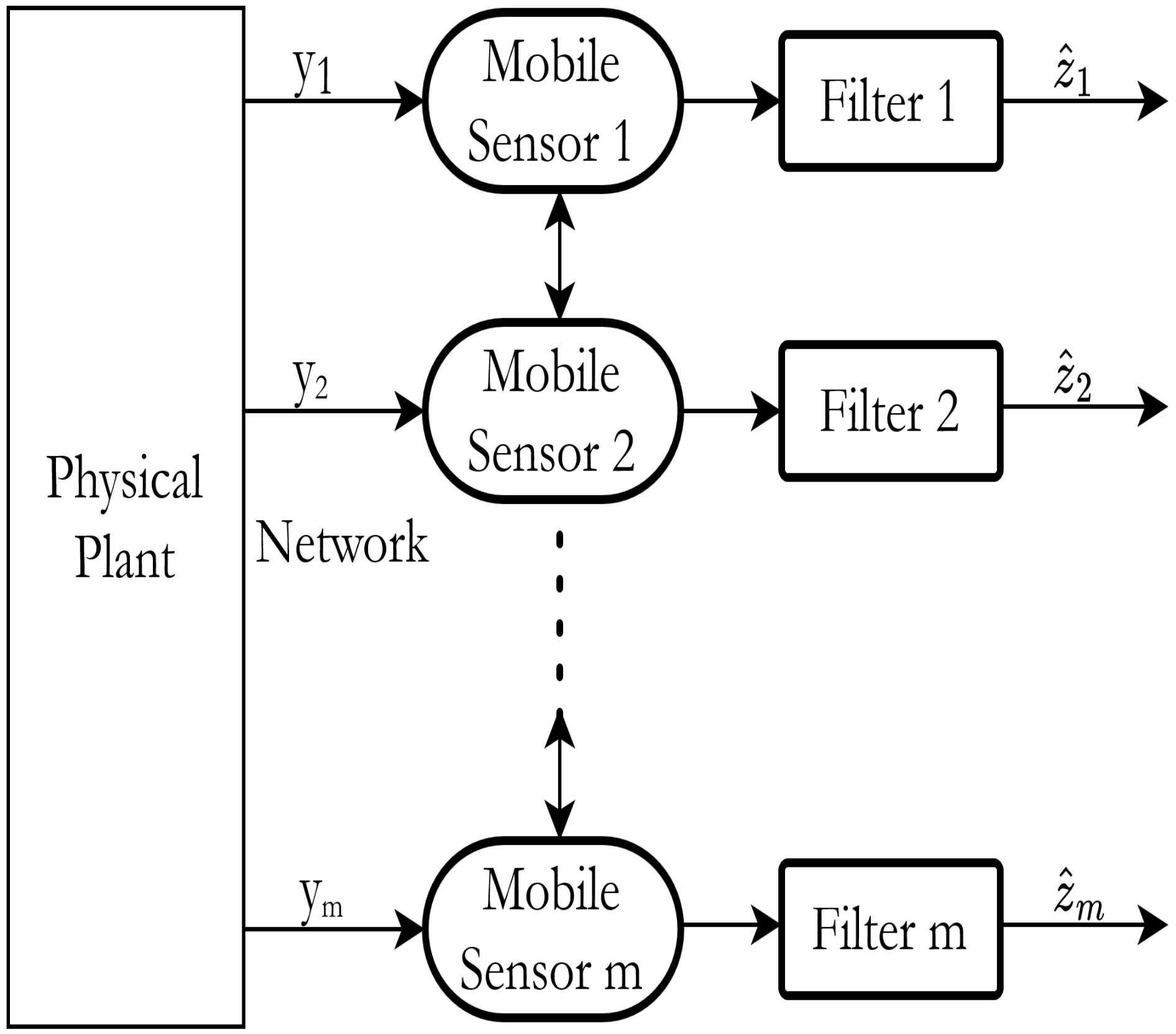
The rest of the manuscript is structured as follows. In Section 2, the 3D nonlinear distributed parameter systems with a network of m mobile sensors is presented; some preliminaries are given. In Section 3, a mobile sensing approach is used to solve the distributed bounded $H_{\infty }$ consensus filter design issue. The discussion of some scenarios related to the main results is available in Section 4. A numerical example is provided in Section 5 to show the effectiveness of the proposed approach. In Section 6, conclusions are drawn.

Notation 1.

The notation is standard, except as otherwise specified. $\dot{\zeta }\left(t\right)$ means the derivative of the function $\zeta \left(t\right)$ with respect to time t. $\mathrm{Prob}\left\{x\right\}$ denotes the probability that event ${}^{\prime }{x}^{\prime }$ will occur. $\mathbb{E}\left\{x\right\}$ stands for the expectation of stochastic variable x. I denotes the identity matrix with appropriate dimension; $\mathrm{diag}\{x_1,x_2,\cdots ,x_m\}$ stands for an m-dimensional diagonal matrix. If M is a matrix, $M^T$ denotes its transpose and ${\lambda }_{max}\left(M\right)$ means the largest eigenvalue of M. Moreover, matrices without explicit dimensions are assumed to be the appropriate dimension ones.

Let $\mathcal{H}$ be a Hilbert space with inner product $\langle ·,·\rangle$ and corresponding induced norm $|·|$. Let $\mathcal{B}$ be a reflexive Banach space with norm denoted by $\parallel ·\parallel$. It is assumed that $\mathcal{B}$ is embedded densely and continuously in $\mathcal{H}$. Let ${\mathcal{B}}^{*}$ denotes the conjugate dual of $\mathcal{B}$ with induced norm ${\parallel ·\parallel }_{*}$. It follows $\mathcal{B}\hookrightarrow \mathcal{H}\hookrightarrow {\mathcal{B}}^{*}$ with both embedding dense and continuously, the result of which is that we have $\left|g\right|\le \varrho \parallel g\parallel ,g\in \mathcal{B}$, for any constant $\varrho >0$ [30].

2. Problem Formulation and Preliminaries

In this paper, a class of 3D nonlinear distributed parameter systems is studied. Let $\eta (t,\zeta )$ denote the state of 3D distributed process at $t\in [0,+\infty )$ and at spatial location $\zeta =({\zeta }_1,{\zeta }_2,{\zeta }_3)\in \Omega$, $where \Omega =\left\{{\zeta }_s\right|0\le {\zeta }_s\le l_s,s=1,2,3\}$ is a bounded region with smooth boundary $\partial \Omega$, and the measure of $\Omega$ is $\mu (\Omega )>0$. The adopted target object can be described by the following 3D nonlinear spatio-temporal distributed process.

$$\left\{\begin{array}{cc}\hfill & \frac{\partial \eta (t,\zeta )}{\partial t}=\sum _{s=1}^3\frac{\partial }{\partial {\zeta }_s}\left(a_s\left({\zeta }_s\right)\frac{\partial \eta (t,\zeta )}{\partial {\zeta }_s}\right)+Hf(t,\eta (t,\zeta ))+d\left(\zeta \right)\nu \left(t\right)\hfill \\ \hfill & z\left(t\right)=\underset{\Omega }{\int \int \int }b\left(\zeta \right)\eta (t,\zeta )d\Omega \hfill \end{array}\right.$$

(1)

subject to the initial condition

$$\eta (0,{\zeta }_1,{\zeta }_2,{\zeta }_3)={\eta }_0({\zeta }_1,{\zeta }_2,{\zeta }_3),$$

(2)

and having Dirichlet boundary conditions

$${\eta (t,0)=0,\eta (t,·)|}_{\partial \Omega }=0,t\ge 0.$$

(3)

The diffusion operators $a_s\left({\zeta }_s\right)\ge {\overline{a}}_s>0,s=1,2,3.$ $d\left(\zeta \right)$ denotes the spatial distribution of perturbation; $\nu \left(t\right)$ is external perturbation; $b\left(\zeta \right)$ is the spatial distribution of the output; H is a negative operator coefficient of nonlinear function $f(t,\eta (t,\zeta \left)\right)$. It is assumed that f can be decomposed into a part $f_L(t,\eta (t,\zeta ))$ that satisfies the sector condition and a part $r(t,\eta (t,\zeta \left)\right)$ that has the saturation property, and these two parts may occur in a probabilistic way.

$$f(t,\eta (t,\zeta ))=\rho \left(t\right)f_L(t,\eta (t,\zeta ))+(1-\rho \left(t\right))r(t,\eta (t,\zeta )),$$

(4)

where the stochastic variable $\rho \left(t\right)\in \mathbf{R}$ is a Bernoulli distributed white sequence taking values of 1 and 0 with

$$\left\{\begin{array}{c}\mathrm{Prob}\{\rho \left(t\right)=1\}=\overline{\rho }\hfill \\ \mathrm{Prob}\{\rho \left(t\right)=0\}=1-\overline{\rho }\hfill \end{array}\right.$$

(5)

where $\overline{\rho }\in [0,1]$ are known positive constant. It is assumed that the stochastic variable $\rho \left(t\right)$ is independent mutually. We have

$$\mathbb{E}\left\{\rho \left(t\right)\right\}=\overline{\rho }\mathrm{and}\mathbb{E}\left\{{(\rho \left(t\right)-\overline{\rho })}^2\right\}=\overline{\rho }(1-\overline{\rho }).$$

(6)

Compared to the Lipschitz condition or sector condition, the decomposition method is another efficient method for dealing with nonlinearities. Also consider the occurrence of the decomposition term in a probabilistic way, the model is more suitable for the effect of environmental nonlinearity in practice.

The measurement output of m mobile sensors in 3D space are presented as follows.

$$y\left(t\right)=\left[\begin{array}{c}{y}_1\left(t\right)\\ y_2\left(t\right)\\ ⋮\\ y_m\left(t\right)\end{array}\right]=\left[\begin{array}{c}{\int \int \int }_{\Omega }{\psi }_1(\zeta ;{\zeta }_1\left(t\right))\eta (t,\zeta )d\Omega \\ {\int \int \int }_{\Omega }{\psi }_2(\zeta ;{\zeta }_2\left(t\right))\eta (t,\zeta )d\Omega \\ ⋮\\ {\int \int \int }_{\Omega }{\psi }_m(\zeta ;{\zeta }_m\left(t\right))\eta (t,\zeta )d\Omega \end{array}\right],$$

(7)

or ith measurement output can be stated as

$$y_i\left(t\right)={\int \int \int }_{\Omega }{\psi }_i(\zeta ;{\zeta }_i\left(t\right))\eta (t,\zeta )d\Omega ,i=1,2,\cdots ,m,$$

(8)

where ${\psi }_i(\zeta ;{\zeta }_i\left(t\right))$ denotes the spatial distribution of ith moving sensing device. The nonnegative function ${\psi }_i(\zeta ;{\zeta }_i\left(t\right))$ is bounded. The spatial distribution function of each mobile sensor, in the general sense, is given by

$${\psi }_i({\zeta }_s;{\zeta }_{is}\left(t\right))=\left\{\begin{array}{c}{\phi }_i\left(\zeta \right)\mathrm{if}\zeta \in {\Omega }_i\hfill \\ 0\mathrm{otherwise},\hfill \end{array}\right.$$

(9)

where ${\zeta }_1\in {\Omega }_{i1}=[{\zeta }_{i1}-{\delta }_{i1},{\zeta }_{i1}+{\delta }_{i1}]$, ${\zeta }_2\in {\Omega }_{i2}=[{\zeta }_{i2}-{\delta }_{i2},{\zeta }_{i2}+{\delta }_{i2}]$, ${\zeta }_3\in {\Omega }_{i3}=[{\zeta }_{i3}-{\delta }_{i3},{\zeta }_{i3}+{\delta }_{i3}]$.

It is worth noting that the spatial distribution here implies that each mobile sensing device can have a different spatial distribution function. $({\zeta }_{i1}\left(t\right),{\zeta }_{i2}\left(t\right),{\zeta }_{i3}\left(t\right))\in [0,l_1]\times [0,l_2]\times [0,l_3]$ denotes the location of the time-varying center of mass of the ith sensing device. Thus, it draws the moving trajectory of the ith sensing device.

The saturation function $\sigma (·):{\mathbf{R}}^r\mapsto {\mathbf{R}}^r$ is defined as

$$\sigma \left(x\right)={[{\sigma }_1^T\left(x_1\right),{\sigma }_2^T\left(x_2\right),\cdots ,{\sigma }_r^T\left(x_r\right)]}^T$$

with ${\sigma }_i\left(x_i\right)=\mathrm{sign}\left(x_i\right)min\{V_{i,max},\mid V_i\mid \}$ where $V_{i,max}$ is the ith element of the vector, and $V_{max}$ is the saturation level.

For every i, the stochastic variable ${ϵ}_i\left(t\right)\in \mathbf{R},i=1,2,\cdots ,m$ is a Bernoulli distributed white sequence taking values of 1 and 0 with

$$\left\{\begin{array}{c}\mathrm{Prob}\{{ϵ}_i\left(t\right)=1\}={\overline{ϵ}}_i\hfill \\ \mathrm{Prob}\{{ϵ}_i\left(t\right)=0\}=1-{\overline{ϵ}}_i\hfill \end{array}\right.$$

(10)

where ${\overline{ϵ}}_i\in [0,1],i=1,2,\cdots ,m$ are known positive constants. It is assumed that the stochastic variables ${ϵ}_i\left(t\right)$ are independent mutually in all $i(1\le i\le m)$. Accordingly, we have

$$\mathbb{E}\{{ϵ}_i\left(t\right)-{\overline{ϵ}}_i\}=0\mathrm{and}\mathbb{E}\left\{{({ϵ}_i\left(t\right)-{\overline{ϵ}}_i)}^2\right\}={\overline{ϵ}}_i(1-{\overline{ϵ}}_i).$$

(11)

The measurement output after considering the randomly occurring sensor saturation can be described as

$${\tilde{y}}_i\left(t\right)={ϵ}_i\left(t\right)y_i\left(t\right)+(1-{ϵ}_i\left(t\right))\sigma \left(y_i\left(t\right)\right),i=1,2,\cdots ,m,$$

(12)

In order to rewrite the 3D nonlinear distributed parameter system (1) as an evolution equation, the following notations are given, and their meanings are explained.

Consider a linear operator $\mathcal{A}:\mathcal{B}\to {\mathcal{B}}^{*}$ satisfying the following assumptions:

Assumption 1.

$\mathcal{A}$ is bounded, that is

$$\left|\langle g,\mathcal{A}h\rangle \right|\le {\epsilon }_0\parallel g\parallel \parallel h\parallel ,$$

for $g,h\in \mathcal{B}$ and constant ${\epsilon }_0>0$.

Assumption 2.

$-\mathcal{A}$ is coercive, that is

$$\langle g,-\mathcal{A}g\rangle \ge {\vartheta }_0{\parallel g\parallel }^2,$$

for $g\in \mathcal{B}$ and constant ${\vartheta }_0>0$.

The operator $\mathcal{A}$ is referred to as state operator. Moreover, the perturbation operator $\mathcal{D}:\mathbf{R}\to {\mathcal{B}}^{*}$ is provided by $\mathcal{D}\nu \left(t\right)=d\left(\zeta \right)\nu \left(t\right)$, which satisfies $\langle g,\mathcal{D}g\rangle \le {\mu }_d\langle g,g\rangle$. For a given time $T_f$, ${\int }_0^{T_f}{\nu }^T\left(t\right)\nu \left(t\right)dt\le {\overline{d}}^2$, where ${\mu }_d,\overline{d}$ are positive constants. In addition, $\mathcal{B}:\mathbf{R}\to {\mathcal{B}}^{*}$ is given by $\langle \mathcal{B}g,h\rangle ={\int \int \int }_{\Omega }b\left(\zeta \right)g\left(\zeta \right)h\left(\zeta \right)d\Omega$, which satisfies $\langle g,\mathcal{B}g\rangle \le {\mu }_b\langle g,g\rangle$.

Then, it can be rewritten to obtain the corresponding compact form of the 3D nonlinear distributed parameter system (1).

$$\left\{\begin{array}{cc}\hfill & \dot{\eta }\left(t\right)=\mathcal{A}\eta \left(t\right)+HF\left(\eta \left(t\right)\right)+\mathcal{D}\nu \left(t\right)\hfill \\ \hfill & z\left(t\right)=\mathcal{B}\eta \left(t\right)\hfill \end{array}\right.$$

(13)

where the state space is $\mathcal{H}=L_2(\Omega )$, where $\eta (t,·)=\left\{\eta \right(t,\zeta ):\zeta \in \Omega \}$ is the state of the system. The space $\mathcal{B}$ is identified by the Sobolev space $\mathcal{B}=H_0^1(0,l)=\{h\in H^1{(\Omega )\left|h\right|}_{\partial \Omega }=0\}$ and its conjugate dual space ${\mathcal{B}}^{*}$ is $H^{-1}(\Omega )$. Let infinitesimal operator $\mathcal{A}={\sum }_{s=1}^3\frac{\partial }{\partial {\zeta }_s}\left(a_s\left({\zeta }_s\right)\frac{\partial \eta (t,\zeta )}{\partial {\zeta }_s}\right)$ and its domain be given by $\mathcal{D}\left(\mathcal{A}\right)=\{h\in L_2(\Omega ):h,h^{\prime }$ are absolutely continuous, $h^{″}\in L_2(\Omega )$ and $h{|}_{\partial \Omega }=0\}$. The infinitesimal operator $\mathcal{A}$ generates a strongly continuous semigroup $T\left(t\right),t\ge 0$, and the domain $\mathcal{D}\left(\mathcal{A}\right)$ of the operator $\mathcal{A}$ is dense in $\mathcal{H}$, [23].

The output can be expressed similarly as

$$\tilde{y}\left(t\right)=ϵ\left(t\right)y\left(t\right)+(I-ϵ\left(t\right))\sigma \left(y\left(t\right)\right),$$

(14)

where $y\left(t\right)=\Psi \left(\zeta \right(t\left)\right)\eta \left(t\right)$, $ϵ\left(t\right)=\mathrm{diag}\{{ϵ}_1\left(t\right),{ϵ}_2\left(t\right),\cdots ,{ϵ}_m\left(t\right)\}$ and output operator $\Psi \left(\zeta \right(t\left)\right)$ is given by

$$\langle \Psi \left(\zeta \left(t\right)\right)g,h\rangle =\left[\begin{array}{c}{\int \int \int }_{\Omega }{\psi }_1(\zeta ;{\zeta }_1\left(t\right))g\left(\zeta \right)h\left(\zeta \right)d\Omega \hfill \\ {\int \int \int }_{\Omega }{\psi }_2(\zeta ;{\zeta }_2\left(t\right))g\left(\zeta \right)h\left(\zeta \right)d\Omega \hfill \\ ⋮\hfill \\ {\int \int \int }_{\Omega }{\psi }_m(\zeta ;{\zeta }_m\left(t\right))g\left(\zeta \right)h\left(\zeta \right)d\Omega \hfill \end{array}\right],$$

where $\Psi \left(\zeta \left(t\right)\right):\mathcal{B}\to \underset{\underset{m}{⏟}}{{\mathbb{R}}^3\times {\mathbb{R}}^3\times \cdots \times {\mathbb{R}}^3}$ satisfying $\langle g,\Psi \left(\zeta \left(t\right)\right)g\rangle \le {\mu }_c\langle g,g\rangle$.

To analyze finite-time $H_{\infty }$ filtering, we consider the following assumptions and definitions.

Assumption 3.

There exists a constant $l_0$ such that

$${(s_1-s_2)}^T(f_L(t,s_1)-f_L(t,s_2))\le l_0{(s_1-s_2)}^T(s_1-s_2)$$

(15)

Assumption 4.

$r(t,\eta (t,\zeta \left)\right)$ is bounded function satisfying

$$\left|r(t,\eta (t,\zeta ))\right|\le r_0,$$

(16)

where $r_0$ is positive constant.

Assumption 5.

The saturation function $\sigma \left(x\right)$ is sector bounded, i.e.,

$${\sigma }^T\left(x\right)\sigma \left(x\right)\le \beta$$

(17)

where β is a positive constant.

Definition 1

(Finite-time stability). For a given time constant $T_f$, 3D filtering error systems with $\nu \left(t\right)=0$ are said to be finite-time stable with respect to $({\alpha }_1,{\alpha }_2,T_f,\mathcal{Q})$ if

$$\langle x\left(t_0\right),\mathcal{Q}x\left(t_0\right)\rangle \le {\alpha }_1^2\Rightarrow \langle x\left(t\right),\mathcal{Q}x\left(t\right)\rangle \le {\alpha }_2^2$$

(18)

where ${\alpha }_2>{\alpha }_1>0$, $\mathcal{Q}$ is a positive definite operator.

Definition 2

(Finite-time boundedness). For a given time constant $T_f$, 3D filtering error systems are said to be finite-time bounded with respect to $({\alpha }_1^2,{\alpha }_2^2,T_f,\overline{d},\mathcal{Q})$ if condition (18) holds, where ${\alpha }_2>{\alpha }_1>0$, $\mathcal{Q}$ is a positive definite operator.

Definition 3

(Distributed bounded $H_{\infty }$ consensus performance). The filters (20) are said to be distributed bounded $H_{\infty }$ consensus filters if there exist $w_0>0$ such that the filtering error ${\tilde{z}}_i\left(t\right)$ satisfy the following inequalities

$$\frac{1}{m}\sum _{i=1}^m|{\tilde{z}}_i{\left(t\right)|}^2\le {\gamma }^2{\left|\nu \left(t\right)\right|}^2+w_0{\alpha }_2^2$$

(19)

where $\gamma >0$ are some given disturbance attenuation level, for any $i\in \{1,2,\cdots ,m\}$. If $w_0=0$, then they are called distributed $H_{\infty }$ consensus filters.

Lemma 1.

Let $x,y$ be any m-dimensional real vectors, and let q be a positive scalar. Then the following inequality holds:

$$2\langle x,y\rangle \le q\langle x,x\rangle +q^{-1}\langle y,y\rangle .$$

3. Main Results

Consider the distributed consensus filter configuration with m mobile sensors as shown in Figure 1, where each sensor can receive information in a distributed way. Being aware of such a fact, we deployed the following filter structure on sensor node i.

$$\left\{\begin{array}{cc}\hfill {\dot{\widehat{\eta }}}_i\left(t\right)=& \mathcal{A}{\widehat{\eta }}_i\left(t\right)+HF\left({\widehat{\eta }}_i\left(t\right)\right)+{\Psi }^{*}\left({\zeta }_i\left(t\right)\right)k_i[{\tilde{y}}_i\left(t\right)-{\overline{ϵ}}_i\Psi \left({\zeta }_i\left(t\right)\right){\widehat{\eta }}_i\left(t\right)]\hfill \\ \hfill & +G_i\kappa \sum _{j=1}^m{\pi }_{ij}{\widehat{\eta }}_j\left(t\right)\hfill \\ \hfill {\widehat{z}}_i\left(t\right)=& \mathcal{B}{\widehat{\eta }}_i\left(t\right)\hfill \end{array}\right.$$

(20)

where ${\widehat{\eta }}_i\left(t\right)$ is the state estimate of ith mobile sensor, and ${\widehat{z}}_i\left(t\right)$ is the estimate for $z\left(t\right)$ from the filter on ith mobile sensor; $k_i>0$ are the observer gains, and $G_i$ are the consensus filter gains. Moreover, $\kappa$ denotes consensus strength coefficient; ${\widehat{\eta }}_i\left(0\right)={\widehat{\eta }}_{i0}\ne \eta \left(0\right)$ for all $i=1,2,\cdots ,m$. $\Pi ={\left({\pi }_{ij}\right)}_{m\times m}$ is irreducible, ${\pi }_{ij}={\pi }_{ji}\ge 0$, for $i\ne j$ and ${\sum }_{j=1}^m{\pi }_{ij}=0$, for all $i=1,2,\cdots ,m$. It is obvious that $\Pi$ has an eigenvalue of zero, and all other eigenvalues are negative.

Letting $e_i\left(t\right)=\eta \left(t\right)-{\widehat{\eta }}_i\left(t\right)$ and ${\tilde{z}}_i\left(t\right)=z\left(t\right)-{\widehat{z}}_i\left(t\right)$, the filtering error system can be presented from (13) and (20) in the following.

$$\left\{\begin{array}{cc}\hfill {\dot{e}}_i\left(t\right)=& \mathcal{A}{e}_i\left(t\right)+H(F\left(\eta \left(t\right)\right)-F\left({\widehat{\eta }}_i\left(t\right)\right))-{\Psi }^{*}\left({\zeta }_i\left(t\right)\right)k_i[{ϵ}_i\left(t\right)y_i\left(t\right)\hfill \\ \hfill & +(1-{ϵ}_i\left(t\right))\sigma \left(y_i\left(t\right)\right)-{\overline{ϵ}}_i\Psi \left({\zeta }_i\left(t\right)\right){\widehat{\eta }}_i\left(t\right)]\hfill \\ \hfill & -G_i\kappa \sum _{j=1}^m{\pi }_{ij}{\widehat{\eta }}_j\left(t\right)+\mathcal{D}\nu \left(t\right)\hfill \\ \hfill {\tilde{z}}_i\left(t\right)=& \mathcal{B}{e}_i\left(t\right)\hfill \end{array}\right.$$

(21)

Then, one can obtain

$$\left\{\begin{array}{cc}\hfill {\dot{e}}_i\left(t\right)=& {\mathcal{A}}_{\psi }\left({\zeta }_i\left(t\right)\right)e_i\left(t\right)+H(F\left(\eta \left(t\right)\right)-F\left({\widehat{\eta }}_i\left(t\right)\right))\hfill \\ \hfill & -{\Psi }^{*}\left({\zeta }_i\left(t\right)\right)k_i({ϵ}_i\left(t\right)-{\overline{ϵ}}_i)\Psi \left({\zeta }_i\left(t\right)\right)\eta \left(t\right)-{\Psi }^{*}\left({\zeta }_i\left(t\right)\right)k_i(1-{ϵ}_i\left(t\right))\sigma \left(y_i\left(t\right)\right)\hfill \\ \hfill & -G_i\kappa \sum _{j=1}^m{\pi }_{ij}{\widehat{\eta }}_j\left(t\right)+\mathcal{D}\nu \left(t\right)\hfill \\ \hfill {\tilde{z}}_i\left(t\right)=& \mathcal{B}{e}_i\left(t\right)\hfill \end{array}\right.$$

(22)

where ${\mathcal{A}}_{\psi }\left({\zeta }_i\left(t\right)\right)=\mathcal{A}-k_i{\overline{ϵ}}_i{\Psi }^{*}\left({\zeta }_i\left(t\right)\right)\Psi \left({\zeta }_i\left(t\right)\right)$.

3.1. Finite-Time Bounded Analysis

Theorem 1.

Under the distributed consensus filter (20) as given, the zero solution of filtering error system (21) is finite-time bounded with respect to $({\alpha }_1^2,{\alpha }_2^2,T_f,\overline{d},{\mathcal{A}}_{\psi }\left({\zeta }_i\left(t\right)\right)$, if there exist positive scalar ${\lambda }_0$, nonnegative constant ϖ and two sets of positive constants $p_i$, $q_i(i=1,2,\cdots ,m)$ such that the following inequalities hold:

$$\begin{array}{cc}\hfill & \overline{\rho }{l}_0+\kappa {\lambda }_{max}(\Pi )<0,\hfill \end{array}$$

(23)

$$\begin{array}{cc}\hfill & {\alpha }_1^2+\widehat{d}\le {\lambda }_0{\alpha }_2^2{e}^{-\varpi T_f}\hfill \end{array}$$

(24)

and the velocity law of mobile sensors as follows:

$${\dot{\zeta }}_{is}\left(t\right)=-c_{is}{k}_i{\overline{ϵ}}_i{\Xi }_{is},s=1,2,3.$$

(25)

where $\widehat{d}=\frac{{\mu }_d^2{\overline{d}}^2}{2}{\sum }_{i=1}^m{q}_i$,

$$\begin{array}{cc}\hfill {\Xi }_{is}=& {\int }_{{\zeta }_{is}-{\delta }_{is}}^{{\zeta }_{is}+{\delta }_{is}}\frac{d{\phi }_i\left({\zeta }_s\right)}{d{\zeta }_s}{\phi }_i\left({\zeta }_s\right)e_i^2(t,\zeta )d{\zeta }_s\hfill \\ \hfill & +{\phi }_i^2({\zeta }_{is}-{\delta }_{is}+0)e_i^2(t,{\zeta }_{is}-{\delta }_{is})-{\phi }_i^2({\zeta }_{is}+{\delta }_{is}+0)e_i^2(t,{\zeta }_{is}+{\delta }_{is}),s=1,2,3.\hfill \end{array}$$

(26)

with $c_{is}>0,s=1,2,3,i=1,2,\cdots ,m$ is velocity gain of each mobile sensor. The guidance strategy for mobile sensors enhances the filter performance in the sense that the filtering error $e_i\left(t\right)$ converges to zero faster. The estimated bound is presented as follows:

$$\begin{array}{cc}\hfill & \underset{t\to \infty }{lim}\frac{1}{m}\mathbb{E}\left(\sum _{i=1}^m{|\eta \left(t\right)-{\widehat{\eta }}_i\left(t\right)|}^2\right)\hfill \\ \hfill & \le {\left(\frac{(1-\overline{\rho })r_0+\sqrt{{(1-\overline{\rho })}^2{r}_0^2-\widehat{\beta }(\overline{\rho }{l}_0+\kappa {\lambda }_{max}(\Pi ))}}{-(\overline{\rho }{l}_0+\kappa {\lambda }_{max}(\Pi ))}\right)}^2,\hfill \end{array}$$

(27)

where $\widehat{\beta }=\frac{\beta {\mu }_c^2}{2m}{\sum }_{i=1}^m{p}_i{k}_i^2{(1-{\overline{ϵ}}_i)}^2$.

Proof. 

Closed-loop spatio-temporal operator ${\mathcal{A}}_{\psi }\left({\zeta }_i\left(t\right)\right)$ is easily verified that it meets

$$\begin{array}{cc}\hfill \left|\sum _{i=1}^m〈g,{\mathcal{A}}_{\psi }\left({\zeta }_i\left(t\right)\right)h〉\right|=& \left|\sum _{i=1}^m〈g,\left(\mathcal{A}-k_i{\overline{ϵ}}_i{\Psi }^{*}\left({\zeta }_i\left(t\right)\right)\Psi \left({\zeta }_i\left(t\right)\right)\right)h〉\right|\hfill \\ \hfill \le & {\epsilon }_{0}m\parallel g\parallel \parallel h\parallel +〈K\overline{ϵ}\Psi \left(\zeta \left(t\right)\right)g,\Psi \left(\zeta \left(t\right)\right)h〉\hfill \\ \hfill \le & {\epsilon }_{0}m\parallel g\parallel \parallel h\parallel +{\lambda }_{max}\left(K\overline{ϵ}\right){\varrho }^2{\mu }^2(\Omega )\parallel g\parallel \parallel h\parallel \hfill \\ \hfill =& {\epsilon }_1\parallel g\parallel \parallel h\parallel \hfill \end{array}$$

(28)

where ${\epsilon }_1={\epsilon }_{0}m+{\lambda }_{max}\left(K\overline{ϵ}\right){\varrho }^2{\mu }^2(\Omega )>0$, $\overline{ϵ}=\mathrm{diag}\{{\overline{ϵ}}_1,{\overline{ϵ}}_2,\cdots ,{\overline{ϵ}}_m\}$, $K=\mathrm{diag}\{k_1,k_2,\cdots ,k_m\}$, $\parallel \Psi \left(\zeta \right(t\left)\right)\parallel =\varrho \mu (\Omega )$.

$$\begin{array}{cc}\hfill \sum _{i=1}^m〈g,-{\mathcal{A}}_{\psi }\left({\zeta }_i\left(t\right)\right)g〉=& \sum _{i=1}^m〈g,-\left(\mathcal{A}-k_i{\overline{ϵ}}_i{\Psi }^{*}\left({\zeta }_i\left(t\right)\right)\Psi \left({\zeta }_i\left(t\right)\right)\right)g〉\hfill \\ \hfill \ge & {\vartheta }_{0}m{\parallel g\parallel }^2+〈K\overline{ϵ}\Psi \left(\zeta \left(t\right)\right)g,\Psi \left(\zeta \left(t\right)\right)g〉\hfill \\ \hfill \ge & {\vartheta }_0{m\parallel g\parallel }^2+{\lambda }_{min}\left(K\overline{ϵ}\right){\left|\Psi \left(\zeta \left(t\right)\right)g\right|}^2\hfill \\ \hfill >& {\vartheta }_{0}m{\parallel g\parallel }^2\hfill \end{array}$$

(29)

where $g,h\in \mathcal{B}$.

By (28) and (29), the linear operator ${\mathcal{A}}_{\psi }\left({\zeta }_i\left(t\right)\right)$ is negative definite and invertible. Thus, we consider the following Lyapunov functional that depends on the spatio-temporal operator ${\mathcal{A}}_{\psi }\left({\zeta }_i\left(t\right)\right)$.

$$V\left(t\right)=-\frac{1}{2}\sum _{i=1}^m\langle e_i\left(t\right),{\mathcal{A}}_{\psi }\left({\zeta }_i\left(t\right)\right)e_i\left(t\right)\rangle .$$

(30)

The infinitesimal operator $\mathcal{L}V$ is defined as $\mathcal{L}V\left(t\right)=\underset{\Delta \to 0^{+}}{lim}\frac{1}{\Delta }[\mathbb{E}\left\{V(t+\Delta )|t\right\}-V\left(t\right)]$, then along the solution of the filtering error system (22), we have

$$\begin{array}{cc}\hfill \mathcal{L}V\left(t\right)=& -\sum _{i=1}^m\mathbb{E}\langle e_i\left(t\right),{\mathcal{A}}_{\psi }\left({\zeta }_i\left(t\right)\right){\dot{e}}_i\left(t\right)\rangle \hfill \\ \hfill & -\frac{1}{2}\sum _{i=1}^m\mathbb{E}〈e_i\left(t\right),\frac{d{\mathcal{A}}_{\psi }\left({\zeta }_i\left(t\right)\right)}{dt}{e}_i\left(t\right)〉.\hfill \end{array}$$

(31)

The following result was simply inferred by taking into account (10)–(12), as well as by noting that the operator ${\mathcal{A}}_{\psi }\left({\zeta }_i\left(t\right)\right)$ is self-adjoint.

$$\begin{array}{cc}\hfill & -\sum _{i=1}^m\mathbb{E}\langle e_i\left(t\right),{\mathcal{A}}_{\psi }\left({\zeta }_i\left(t\right)\right){\dot{e}}_i\left(t\right)\rangle \hfill \\ \hfill =& -\sum _{i=1}^m\mathbb{E}\langle e_i\left(t\right),{\mathcal{A}}_{\psi }\left({\zeta }_i\left(t\right)\right){\mathcal{A}}_{\psi }\left({\zeta }_i\left(t\right)\right)e_i\left(t\right)\rangle \hfill \\ \hfill & -\sum _{i=1}^m\mathbb{E}\langle e_i\left(t\right),{\mathcal{A}}_{\psi }\left({\zeta }_i\left(t\right)\right)H(F\left(\eta \left(t\right)\right)-F\left({\widehat{\eta }}_i\left(t\right)\right))\rangle \hfill \\ \hfill & +\sum _{i=1}^m\mathbb{E}\langle e_i\left(t\right),{\mathcal{A}}_{\psi }\left({\zeta }_i\left(t\right)\right){\Psi }^{*}\left({\zeta }_i\left(t\right)\right)k_i({ϵ}_i\left(t\right)-{\overline{ϵ}}_i)\Psi \left({\zeta }_i\left(t\right)\right)\eta \left(t\right)\rangle \hfill \\ \hfill & +\sum _{i=1}^m\mathbb{E}\langle e_i\left(t\right),{\mathcal{A}}_{\psi }\left({\zeta }_i\left(t\right)\right){\Psi }^{*}\left({\zeta }_i\left(t\right)\right)k_i(1-{ϵ}_i\left(t\right))\sigma \left(y_i\left(t\right)\right)\rangle \hfill \\ \hfill & +\sum _{i=1}^m〈e_i\left(t\right),{\mathcal{A}}_{\psi }\left({\zeta }_i\left(t\right)\right)G_i\kappa \sum _{j=1}^m{\pi }_{ij}{e}_j\left(t\right)〉\hfill \\ \hfill & -\sum _{i=1}^m\langle e_i\left(t\right),{\mathcal{A}}_{\psi }\left({\zeta }_i\left(t\right)\right)\mathcal{D}\nu \left(t\right)\rangle \hfill \end{array}$$

(32)

By Assumptions 3 and 4 together with (4)–(6), the following holds:

$$\begin{array}{cc}\hfill & -\sum _{i=1}^m\mathbb{E}\langle e_i\left(t\right),{\mathcal{A}}_{\psi }\left({\zeta }_i\left(t\right)\right)H(F\left(\eta \left(t\right)\right)-F\left({\widehat{\eta }}_i\left(t\right)\right))\rangle \hfill \\ \hfill =& \sum _{i=1}^m\mathbb{E}\langle e_i\left(t\right),F\left(\eta \left(t\right)\right)-F\left({\widehat{\eta }}_i\left(t\right)\right)\rangle \hfill \\ \hfill \le & \overline{\rho }{l}_0\sum _{i=1}^m|e_i{\left(t\right)|}^2+2(1-\overline{\rho })r_0\sum _{i=1}^m\left|e_i\left(t\right)\right|\hfill \end{array}$$

(33)

where $H=-{\mathcal{A}}_{\psi }^{-1}\left({\zeta }_i\left(t\right)\right)$.

Here, selecting the consensus filter gains $G_i={\mathcal{A}}_{\psi }^{-1}\left({\zeta }_i\left(t\right)\right)$ out of simplicity, we obtain

$$\begin{array}{cc}\hfill & \sum _{i=1}^m〈e_i\left(t\right),{\mathcal{A}}_{\psi }\left({\zeta }_i\left(t\right)\right)G_i\kappa \sum _{j=1}^m{\pi }_{ij}{e}_j\left(t\right)〉\hfill \\ \hfill =& \kappa \sum _{i=1}^m〈e_i\left(t\right),\sum _{j=1}^m{\pi }_{ij}{e}_j\left(t\right)〉\hfill \\ \hfill =& \kappa \sum _{i=1}^m\sum _{j=1}^m{\pi }_{ij}{\left|e_i\left(t\right)\right|}^2\hfill \end{array}$$

(34)

Moreover, it is simple to deduce that

$$\begin{array}{cc}\hfill & -\sum _{i=1}^m\mathbb{E}\langle e_i\left(t\right),{\mathcal{A}}_{\psi }\left({\zeta }_i\left(t\right)\right)\mathcal{D}\nu \left(t\right)\rangle \hfill \\ \hfill \le & \sum _{i=1}^m\frac{q_i}{2}\langle \mathcal{D}\nu \left(t\right),\mathcal{D}\nu \left(t\right)\rangle +\sum _{i=1}^m\frac{1}{2q_i}\langle {\mathcal{A}}_{\psi }\left({\zeta }_i\left(t\right)\right)e_i\left(t\right),{\mathcal{A}}_{\psi }\left({\zeta }_i\left(t\right)\right)e_i\left(t\right)\rangle \hfill \\ \hfill \le & \sum _{i=1}^m\frac{q_i}{2}{\mu }_d^2{\left|\nu \left(t\right)\right|}^2+\sum _{i=1}^m\frac{1}{2q_i}{\left|{\mathcal{A}}_{\psi }\left({\zeta }_i\left(t\right)\right)e_i\left(t\right)\right|}^2\hfill \end{array}$$

(35)

By Lemma 1, the following holds:

$$\begin{array}{cc}\hfill & \sum _{i=1}^m\mathbb{E}\langle e_i\left(t\right),{\mathcal{A}}_{\psi }\left({\zeta }_i\left(t\right)\right){\Psi }^{*}\left({\zeta }_i\left(t\right)\right)k_i(1-{ϵ}_i\left(t\right))\sigma \left(y_i\left(t\right)\right)\rangle \hfill \\ \hfill \le & \sum _{i=1}^m\frac{p_i}{2}\mathbb{E}\langle {\Psi }^{*}\left({\zeta }_i\left(t\right)\right)k_i(1-{ϵ}_i\left(t\right))\sigma \left(y_i\left(t\right)\right),{\Psi }^{*}\left({\zeta }_i\left(t\right)\right)k_i(1-{ϵ}_i\left(t\right))\sigma \left(y_i\left(t\right)\right))\rangle \hfill \\ \hfill & +\sum _{i=1}^m\frac{1}{2p_i}\mathbb{E}\langle {\mathcal{A}}_{\psi }\left({\zeta }_i\left(t\right)\right)e_i\left(t\right),{\mathcal{A}}_{\psi }\left({\zeta }_i\left(t\right)\right)e_i\left(t\right)\rangle \hfill \\ \hfill \le & {\mu }_c^2\sum _{i=1}^m\frac{p_i{k}_i^2{(1-{\overline{ϵ}}_i)}^2}{2}\langle \sigma \left(y_i\left(t\right)\right),\sigma \left(y_i\left(t\right)\right)\rangle +\sum _{i=1}^m\frac{1}{2p_i}{\left|{\mathcal{A}}_{\psi }\left({\zeta }_i\left(t\right)\right)e_i\left(t\right)\right|}^2\hfill \end{array}$$

(36)

Substituting (34)–(37) into (33) leads to

$$\begin{array}{cc}\hfill & -\sum _{i=1}^m\mathbb{E}\langle e_i\left(t\right),{\mathcal{A}}_{\psi }\left({\zeta }_i\left(t\right)\right){\dot{e}}_i\left(t\right)\rangle \hfill \\ \hfill \le & -\sum _{i=1}^m{\left|{\mathcal{A}}_{\psi }\left({\zeta }_i\left(t\right)\right)e_i\left(t\right)\right|}^2\hfill \\ \hfill & +\overline{\rho }{l}_0\sum _{i=1}^m|e_i{\left(t\right)|}^2+2(1-\overline{\rho })r_0\sum _{i=1}^m\left|e_i\left(t\right)\right|\hfill \\ \hfill & +{\mu }_c^2\sum _{i=1}^m\frac{p_i{k}_i^2{(1-{\overline{ϵ}}_i)}^2}{2}\langle \sigma \left(y_i\left(t\right)\right),\sigma \left(y_i\left(t\right)\right)\rangle +\sum _{i=1}^m\frac{1}{2p_i}{\left|{\mathcal{A}}_{\psi }\left({\zeta }_i\left(t\right)\right)e_i\left(t\right)\right|}^2\hfill \\ \hfill & +\kappa \sum _{i=1}^m\sum _{j=1}^m{\pi }_{ij}{\left|e_i\left(t\right)\right|}^2\hfill \\ \hfill & +\sum _{i=1}^m\frac{q_i}{2}{\mu }_d^2{\left|\nu \left(t\right)\right|}^2+\sum _{i=1}^m\frac{1}{2q_i}{\left|{\mathcal{A}}_{\psi }\left({\zeta }_i\left(t\right)\right)e_i\left(t\right)\right|}^2\hfill \\ \hfill \le & \sum _{i=1}^m\left(-1+\frac{1}{2p_i}+\frac{1}{2q_i}\right){\left|{\mathcal{A}}_{\psi }\left({\zeta }_i\left(t\right)\right)e_i\left(t\right)\right|}^2\hfill \\ \hfill & +(\overline{\rho }{l}_0+\kappa {\lambda }_{max}(\Pi ))\sum _{i=1}^m|e_i{\left(t\right)|}^2+2(1-\overline{\rho })r_0\sum _{i=1}^m\left|e_i\left(t\right)\right|\hfill \\ \hfill & +{\mu }_c^2\sum _{i=1}^m\frac{p_i{k}_i^2{(1-{\overline{ϵ}}_i)}^2}{2}\beta +\sum _{i=1}^m\frac{q_i}{2}{\mu }_d^2{\overline{d}}^2\hfill \end{array}$$

(37)

Furthermore, with respect to the second part of (32), we obtain

$$\begin{array}{cc}\hfill & -\frac{1}{2}\sum _{i=1}^m\mathbb{E}〈e_i\left(t\right),\frac{d{\mathcal{A}}_{\psi }\left({\zeta }_i\left(t\right)\right)}{dt}{e}_i\left(t\right)〉\hfill \\ \hfill =& \frac{1}{2}\sum _{i=1}^m{k}_i{\overline{ϵ}}_i〈e_i\left(t\right),\frac{d{\Psi }^{*}\left({\zeta }_i\left(t\right)\right)\Psi \left({\zeta }_i\left(t\right)\right)}{dt}{e}_i\left(t\right)〉\hfill \\ \hfill =& \sum _{s=1}^3\sum _{i=1}^m{k}_i{\overline{ϵ}}_i〈{\psi }_i\left({\zeta }_{is}\left(t\right)\right)e_i\left(t\right),{\dot{\zeta }}_{is}\left(t\right))\frac{d{\psi }_i\left({\zeta }_{is}\left(t\right)\right)}{d{\zeta }_s}{e}_i\left(t\right)〉\hfill \\ \hfill =& \sum _{s=1}^3\sum _{i=1}^m{k}_i{\overline{ϵ}}_i{\dot{\zeta }}_{is}\left(t\right)){\int }_0^{l_{is}}{\phi }_i\left({\zeta }_s\right)\frac{d{\phi }_i\left({\zeta }_s\right)}{d{\zeta }_s}{e}_i^2\left(t\right)d{\zeta }_s\hfill \\ \hfill =& \sum _{i=1}^m{k}_i{\overline{ϵ}}_i{\dot{\zeta }}_{is}\left(t\right)\sum _{s=1}^3{\Xi }_{is}\hfill \end{array}$$

(38)

where ${\Xi }_{is},s=1,2,3$ have been defined in Theorem 1.

The choice

$${\dot{\zeta }}_{is}\left(t\right)=-c_{is}{k}_i{\overline{ϵ}}_i{\Xi }_{is},s=1,2,3.$$

(39)

Deduce (39) negative definite, $c_{is}>0,s=1,2,3;i=1,2,\cdots ,m.$ Notice that $({\dot{\zeta }}_{i1}\left(t\right),{\dot{\zeta }}_{i2}\left(t\right),{\dot{\zeta }}_{i3}\left(t\right))$ is the velocity of ith moving sensing device.

Subsequently, from (38) and (39), it follows that:

$$\begin{array}{cc}\hfill \mathcal{L}V\left(t\right)\le & \sum _{i=1}^m{\varpi }_i{\left|{\mathcal{A}}_{\psi }\left({\zeta }_i\left(t\right)\right)e_i\left(t\right)\right|}^2+\widehat{d}\hfill \\ \hfill & +\left(\overline{\rho }{l}_0+\kappa {\lambda }_{max}(\Pi )\right)\sum _{i=1}^m{\left|e_i\left(t\right)\right|}^2\hfill \\ \hfill & +2(1-\overline{\rho })r_0\sum _{i=1}^m\left|e_i\left(t\right)\right|+\frac{\beta {\mu }_c^2}{2}\sum _{i=1}^m{p}_i{k}_i^2{(1-{\overline{ϵ}}_i)}^2\hfill \end{array}$$

(40)

where ${\varpi }_i=-1+\frac{1}{2p_i}+\frac{1}{2q_i}$ and $\widehat{d}$ is defined in Theorem 1.

Note that

$$\begin{array}{cc}\hfill {\left(\sum _{i=1}^m\left|e_i\left(t\right)\right|\right)}^2=& \sum _{i=1}^m\sum _{j=1}^m|e_i\left(t\right)\left|\right|e_j\left(t\right)|\hfill \\ \hfill \le & \frac{1}{2}\sum _{i=1}^m\sum _{j=1}^m\left(|e_i{\left(t\right)|}^2+{\left|e_j\left(t\right)\right|}^2\right)\hfill \\ \hfill =& m\sum _{i=1}^m{\left|e_i\left(t\right)\right|}^2\hfill \end{array}$$

(41)

Then, it follows that

$$\begin{array}{cc}\hfill \mathcal{L}V\left(t\right)\le & {\varpi }_0\sum _{i=1}^m{\left|{\mathcal{A}}_{\psi }\left({\zeta }_i\left(t\right)\right)e_i\left(t\right)\right|}^2+\widehat{d}\hfill \\ \hfill & +\left(\overline{\rho }{l}_0+\kappa {\lambda }_{max}(\Pi )\right)\sum _{i=1}^m{\left|e_i\left(t\right)\right|}^2\hfill \\ \hfill & +2(1-\overline{\rho })r_0\sqrt{m}\sqrt{\sum _{i=1}^m{\left|e_i\left(t\right)\right|}^2}+\frac{\beta {\mu }_c^2}{2}\sum _{i=1}^m{p}_i{k}_i^2{(1-{\overline{ϵ}}_i)}^2\hfill \\ \hfill <& \varpi V\left(t\right)+\widehat{d}\hfill \\ \hfill & +\left(\overline{\rho }{l}_0+\kappa {\lambda }_{max}(\Pi )\right)m[\frac{1}{m}\sum _{i=1}^m{\left|e_i\left(t\right)\right|}^2\hfill \\ \hfill & +\frac{2(1-\overline{\rho })r_0}{\overline{\rho }{l}_0+\kappa {\lambda }_{max}(\Pi )}\sqrt{\frac{1}{m}\sum _{i=1}^m{\left|e_i\left(t\right)\right|}^2}\hfill \\ \hfill & -\frac{\widehat{\beta }}{-\left(\overline{\rho }{l}_0+\kappa {\lambda }_{max}(\Pi )\right)}].\hfill \end{array}$$

(42)

where ${\varpi }_0=max\left\{{\varpi }_i\right\},i=1,2,\cdots ,m$, $\varpi =2{\varpi }_0{\vartheta }_{0}m$ and $\widehat{\beta }$ is defined in Theorem 1. Let $\chi =\sqrt{\frac{1}{m}{\sum }_{i=1}^m{\left|e_i\left(t\right)\right|}^2}$ and $w\left(\chi \right)={\chi }^2+\frac{2(1-\overline{\rho })r_0}{\overline{\rho }{l}_0+\kappa {\lambda }_{max}(\Pi )}\chi -\frac{\widehat{\beta }}{-\left(\overline{\rho }{l}_0+\kappa {\lambda }_{max}(\Pi )\right)}$. It is simple to observe that $w\left(x\right)=0$ has two solutions

$${\chi }_{1,2}=\frac{-(1-\overline{\rho })r_0\pm \sqrt{{(1-\overline{\rho })}^2{r}_0^2-\widehat{\beta }(\overline{\rho }{l}_0+\kappa {\lambda }_{max}(\Pi ))}}{\overline{\rho }{l}_0+\kappa {\lambda }_{max}(\Pi )}$$

(43)

where ${\chi }_1<0$ and ${\chi }_2>0$. If $\chi \ge {\chi }_2$, then $w\left(\chi \right)\ge 0$.

Thus, it is not difficult to draw the following conclusion

$$\mathcal{L}V\left(t\right)<\varpi V\left(t\right)+\widehat{d}.$$

(44)

From (45), we can conclude that

$$\begin{array}{cc}\hfill V\left(t\right)<& e^{\varpi T_f}\left(V\left(0\right)+m\widehat{d}\right)\hfill \\ \hfill =& e^{\varpi T_f}\left(-\frac{1}{2}\sum _{i=1}^m\langle e_i\left(0\right),{\mathcal{A}}_{\psi }\left({\zeta }_i\left(t\right)\right)e_i\left(0\right)\rangle +m\widehat{d}\right)\hfill \\ \hfill <& e^{\varpi T_f}m\left({\alpha }_1^2+\widehat{d}\right).\hfill \end{array}$$

(45)

From the definition of $V\left(t\right)$, there exists $0<{\lambda }_0\le \frac{1}{2}$ such that

$$V\left(t\right)\ge -{\lambda }_0\sum _{i=1}^m\langle e_i\left(t\right),{\mathcal{A}}_{\psi }\left({\zeta }_i\left(t\right)\right)e_i\left(t\right)\rangle$$

(46)

Therefore, we obtain

$$\begin{array}{cc}\hfill -\sum _{i=1}^m\langle e_i\left(t\right),{\mathcal{A}}_{\psi }\left({\zeta }_i\left(t\right)\right)e_i\left(t\right)\rangle <& \frac{1}{{\lambda }_0}{e}^{\varpi T_f}m\left({\alpha }_1^2+\widehat{d}\right)\hfill \\ \hfill \le & m{\alpha }_2^2.\hfill \end{array}$$

(47)

This completes the proof.  □

3.2. Distributed $H_{\infty }$ Consensus Performance Analysis

Next, we will concentrate on studying the $H_{\infty }$ performance of the zero initial condition for the filtering error system (21).

Theorem 2.

Let the filter parameter $k_i$ and $G_i$ and the perturbation attenuation level $\gamma >0$ be given. Then, the zero solution of the filtering error system (21) is finite-time bounded with respect to $(0,{\alpha }_2^2,T_f,\overline{d},{\mathcal{A}}_{\psi }\left({\zeta }_i\left(t\right)\right))$, and $\tilde{z}$ satisfies the bounded $H_{\infty }$ consensus performance constraint (19) under the zero initial condition for all nonzero $\nu \left(t\right)$, if under Assumptiosns 1–5 such that the following inequalities hold:

$$\begin{array}{cc}\hfill & \overline{\rho }{l}_0+\kappa {\lambda }_{max}(\Pi )+{\mu }_b^2<0,\hfill \end{array}$$

(48)

$$\begin{array}{cc}\hfill & -\gamma +\frac{{\mu }_d^2}{2m}\sum _{i=1}^m{q}_i<0,\hfill \end{array}$$

(49)

and the velocity law of mobile sensor is determined as (25) and (26). The estimated bound is given by

$$\begin{array}{cc}\hfill & \underset{t\to \infty }{lim}\frac{1}{m}\mathbb{E}\left(\sum _{i=1}^m{|\eta \left(t\right)-{\widehat{\eta }}_i\left(t\right)|}^2\right)\hfill \\ \hfill & \le {\left(\frac{(1-\overline{\rho })r_0+\sqrt{{(1-\overline{\rho })}^2{r}_0^2-\widehat{\beta }{l}_1}}{-l_1}\right)}^2.\hfill \end{array}$$

(50)

Proof. 

It is simple to prove that (23)–(25) implies the filtering error system (21) is finite-time bounded. The $H_{\infty }$ consensus performance of the closed-loop system will now be the subject of our discussion. The same functional Lyapunov candidate $V\left(t\right)$ from Theorem 1 should be built. As in Theorem 1, similar line calculation yields

$$\mathcal{L}V\left(t\right)\le \frac{\varpi m}{2}{\alpha }_2^2+\left(\overline{\rho }{l}_0+\kappa {\lambda }_{max}(\Pi )\right)mw\left(\chi \right)+\widehat{d}.$$

(51)

In order to address the system’s $H_{\infty }$ consensus performance (19), we establish

$$\begin{array}{cc}\hfill J=& \mathbb{E}\sum _{i=1}^m{\int }_0^{T_f}|{\tilde{z}}_i{\left(t\right)|}^2-{\gamma }^2{\left|\nu \left(t\right)\right|}^{2}dt\hfill \\ \hfill =& \mathbb{E}\sum _{i=1}^m{\int }_0^{T_f}\langle {\tilde{z}}_i\left(t\right),{\tilde{z}}_i\left(t\right)\rangle dt-m{\gamma }^2{\int }_0^{T_f}\langle \nu \left(t\right),\nu \left(t\right)\rangle dt.\hfill \end{array}$$

(52)

From (45) to (46), with the zero initial condition, we have

$$\begin{array}{cc}\hfill J\le & {\int }_0^{T_f}\sum _{i=1}^m\langle \mathcal{B}{e}_i\left(t\right),\mathcal{B}{e}_i\left(t\right)\rangle dt-m{\gamma }^2{\overline{d}}^2+\mathcal{L}V\left(t\right)\hfill \\ \hfill \le & \frac{\varpi m}{2}{\alpha }_2^2+l_{1}m\tilde{w}\left(\chi \right)+\check{d},\hfill \end{array}$$

(53)

where $l_1=\overline{\rho }{l}_0+\kappa {\lambda }_{max}(\Pi )+{\mu }_b^2$, $\tilde{w}\left(\chi \right)={\chi }^2+\frac{2(1-\overline{\rho })r_0}{l_1}\chi -\frac{\widehat{\beta }}{-l_1}$ and $\check{d}=(-{\gamma }^2+\frac{{\mu }_d^2}{2m}{\sum }_{i=1}^m{q}_i)m{\overline{d}}^2$.

It is easy to see that $\tilde{w}\left(\chi \right)=0$ has two solutions

$${\chi }_{1,2}=\frac{-(1-\overline{\rho })r_0\pm \sqrt{{(1-\overline{\rho })}^2{r}_0^2-\widehat{\beta }{l}_1}}{l_1},$$

(54)

where ${\chi }_1<0$ and ${\chi }_2>0$. If $\chi \ge {\chi }_2$, then $\tilde{w}\left(\chi \right)>0$. It is known with the condition (48) and (49) that $l_{1}m\tilde{w}\left(\chi \right)+\check{d}<0$.

Letting $T_f\to \infty$, we obtain that

$$\sum _{i=1}^m{\int }_0^{T_f}\langle {\tilde{z}}_i\left(t\right),{\tilde{z}}_i\left(t\right)\rangle dt<m{\gamma }^2{\int }_0^{T_f}\langle \nu \left(t\right),\nu \left(t\right)\rangle dt+\frac{\varpi m}{2}{\alpha }_2^2,$$

namely,

$$\frac{1}{m}\sum _{i=1}^m|{\tilde{z}}_i{\left(t\right)|}^2<{\gamma }^2{\left|\nu \left(t\right)\right|}^2+\frac{\varpi }{2}{\alpha }_2^2,$$

which completes the proof of the theorem.  □

Remark 1.

A distributed consensus filter is built in (20) based on the mobile sensing approach. The filter can be adapted to the state estimation of complex environments. On the one hand, the nonlinear function in the system is assumed to have two parts, including the part that satisfies the sector condition and the part with saturation characteristics, and both parts occurred randomly. On the other hand, the randomly occurring saturation is considered at the output measurement. This leads to a better robustness of the filter.

Remark 2.

From (27), it follows that the minimal bound increases as $r_0$ or β increases. Thus, a very large filter gain should not be used if the bounds $r_0$ or β of the saturation is relatively high.

4. Discussion

Because of the generality of the conclusion given in Theorem 1, we discuss a few special scenarios of its application in the following.

4.1. Measurement Output with Saturation

If the measurement output is sensor saturation, the output can be expressed as

$${\check{y}}_i\left(t\right)=\sigma \left({\int \int \int }_{\Omega }{\psi }_i(\zeta ;{\zeta }_i\left(t\right))\eta (t,\zeta )d\Omega \right),i=1,2,\cdots ,m.$$

(55)

Its abstract form is

$$\check{y}\left(t\right)=\sigma \left(\Psi \left(\zeta \left(t\right)\right)\eta \left(t\right)\right).$$

(56)

Since the saturation function has obvious nonlinear characteristics, with the help of techniques for dealing with nonlinear terms in the system, we can decompose the saturation function into a sector nonlinear part and a high-order saturation part to facilitate our analysis.

$$\sigma \left(y\left(t\right)\right)=C_1\Psi \left(\zeta \left(t\right)\right)\eta \left(t\right)+R\left(y\left(t\right)\right).$$

(57)

Considering Assumption 4, the high-order saturation part $R\left(y\right(t\left)\right)$ satisfies

$$\left|R\left(y\left(t\right)\right)\right|\le r_1.$$

(58)

For the nonlinear function f of the 3D system, take $\overline{\rho }=1$; hence $f(t,\eta (t,\zeta ))=f_L(t,\eta (t,\zeta ))$ satisfies Assumption 3.

To study the distributed $H_{\infty }$ consensus filtering of the 3D nonlinear distributed parameter systems with sensor saturation, the distributed consensus filters (20) can be modified to the following form.

$$\left\{\begin{array}{cc}\hfill {\dot{\widehat{\eta }}}_i\left(t\right)=& \mathcal{A}{\widehat{\eta }}_i\left(t\right)+HF\left({\widehat{\eta }}_i\left(t\right)\right)+{\Psi }^{*}\left({\zeta }_i\left(t\right)\right)k_i[{\check{y}}_i\left(t\right)-C_1\Psi \left({\zeta }_i\left(t\right)\right){\widehat{\eta }}_i\left(t\right)]\hfill \\ \hfill & +G_i\kappa \sum _{j=1}^m{\pi }_{ij}{\widehat{\eta }}_j\left(t\right)\hfill \\ \hfill {\widehat{z}}_i\left(t\right)=& \mathcal{B}{\widehat{\eta }}_i\left(t\right)\hfill \end{array}\right.$$

(59)

The filtering error system can be given from (13) and (59) as follows.

$$\left\{\begin{array}{cc}\hfill {\dot{e}}_i\left(t\right)=& {\tilde{\mathcal{A}}}_{\psi }{e}_i\left(t\right)+H(F\left(\eta \left(t\right)\right)-F\left({\widehat{\eta }}_i\left(t\right)\right))-{\Psi }^{*}\left({\zeta }_i\left(t\right)\right)k_{i}R\left(y_i\left(t\right)\right)\hfill \\ \hfill & -G_i\kappa \sum _{j=1}^m{\pi }_{ij}{\widehat{\eta }}_j\left(t\right)+\mathcal{D}\nu \left(t\right)\hfill \\ \hfill {\tilde{z}}_i\left(t\right)=& \mathcal{B}{e}_i\left(t\right)\hfill \end{array}\right.$$

(60)

where ${\tilde{\mathcal{A}}}_{\psi }\left({\zeta }_i\left(t\right)\right)=\mathcal{A}-k_i{C}_1{\Psi }^{*}\left({\zeta }_i\left(t\right)\right)\Psi \left({\zeta }_i\left(t\right)\right)$.

Similar to the proof of Theorem 1, let the Lyapunov function $V\left(t\right)=-\frac{1}{2}{\sum }_{i=1}^m\langle e_i\left(t\right),{\tilde{\mathcal{A}}}_{\psi }\left({\zeta }_i\left(t\right)\right)e_i\left(t\right)\rangle$ here. The following inequality

$$\begin{array}{c}\hfill \sum _{i=1}^m\langle e_i\left(t\right),{\tilde{\mathcal{A}}}_{\psi }\left({\zeta }_i\left(t\right)\right){\Psi }^{*}\left({\zeta }_i\left(t\right)\right)k_{i}R\left(y_i\left(t\right)\right)\rangle \le -r_1\sum _{i=1}^m{\tilde{\vartheta }}_i{k}_i\left|e_i\left(t\right)\right|\end{array}$$

where ${\tilde{\vartheta }}_i=({\vartheta }_0+k_i{l}_1{\mu }^2(\Omega ))\mu (\Omega )$, are available when dealing with this Lyapunov functional.

Thus, it follows that

$$\begin{array}{cc}\hfill \mathcal{L}V\left(t\right)\le & {\varpi }_m\sum _{i=1}^m{\left|{\tilde{\mathcal{A}}}_{\psi }\left({\zeta }_i\left(t\right)\right)e_i\left(t\right)\right|}^2+\widehat{d}\hfill \\ \hfill & +\left(l_0+\kappa {\lambda }_{max}(\Pi )\right)\sum _{i=1}^m{\left|e_i\left(t\right)\right|}^2\hfill \\ \hfill & -r_1{\lambda }_{max}\left(\tilde{\Theta }K\right)\sum _{i=1}^m\left|e_i\left(t\right)\right|+\widehat{\beta },\hfill \end{array}$$

(61)

where $\tilde{\Theta }=\mathrm{diag}\{{\tilde{\vartheta }}_1,{\tilde{\vartheta }}_2,\cdots ,{\tilde{\vartheta }}_m\}$.

From the above, it is not difficult to draw the following corollary.

Corollary 1.

Let the filter parameter $k_i$ and $G_i$ and the perturbation attenuation level $\gamma >0$ be given. Then, the zero solution of the filtering error system (60) is finite-time bounded with respect to $(0,{\alpha }_2^2,T_f,\overline{d},{\mathcal{A}}_{\psi }\left({\zeta }_i\left(t\right)\right))$, and $\tilde{z}$ satisfies the bounded $H_{\infty }$ consensus performance constraint (19) under the zero initial condition for all nonzero $\nu \left(t\right)$, if under Assumptions 1–5 such that the following inequalities hold:

$$\begin{array}{cc}\hfill & l_0+\kappa {\lambda }_{max}(\Pi )+{\mu }_b^2<0,\hfill \end{array}$$

(62)

$$\begin{array}{cc}\hfill & -\gamma +\frac{{\mu }_d^2}{2m}\sum _{i=1}^m{q}_i<0,\hfill \end{array}$$

(63)

and the velocity law of the mobile sensor is determined as (25) and (26). The estimated bound is given by

$$\begin{array}{cc}\hfill & \underset{t\to \infty }{lim}\frac{1}{m}\mathbb{E}\left(\sum _{i=1}^m{|\eta \left(t\right)-{\widehat{\eta }}_i\left(t\right)|}^2\right)\hfill \\ \hfill & \le {\left(\frac{r_1{\lambda }_{max}\left(\tilde{\Theta }K\right)+\sqrt{r_1^2{\lambda }_{max}^2\left(\tilde{\Theta }K\right)-4\widehat{\beta }{\widehat{l}}_1}}{-2{\widehat{l}}_1}\right)}^2.\hfill \end{array}$$

(64)

where ${\widehat{l}}_1=l_0+\kappa {\lambda }_{max}(\Pi )+{\mu }_b^2$.

4.2. Measurement Output with Packet Losses

If sensor saturation is not taken into account in the measurement output, then the stochastic variable ${ϵ}_i\left(t\right)$ in the output expression (65) implies the scenario of missing data in the measurement output.

$${\overline{y}}_i\left(t\right)={ϵ}_i\left(t\right){\int \int \int }_{\Omega }{\psi }_i(\zeta ;{\zeta }_i\left(t\right))\eta (t,\zeta )d\Omega ,i=1,2,\cdots ,m.$$

(65)

Its abstract form can be expressed as

$$\overline{y}\left(t\right)=ϵ\left(t\right)\Psi \left(\zeta \left(t\right)\right)\eta \left(t\right).$$

(66)

For the nonlinear function f of the 3D system, take $\overline{\rho }=0$; hence $f(t,\eta (t,\zeta \left)\right)=r(t,\eta (t,\zeta \left)\right)$ satisfies Assumption 4.

Combined with the output (66), a modified distributed filter can be written as

$$\left\{\begin{array}{cc}\hfill {\dot{\widehat{\eta }}}_i\left(t\right)=& \mathcal{A}{\widehat{\eta }}_i\left(t\right)+HF\left({\widehat{\eta }}_i\left(t\right)\right)+{\Psi }^{*}\left({\zeta }_i\left(t\right)\right)k_i[{\overline{y}}_i\left(t\right)-{\overline{ϵ}}_i\Psi \left({\zeta }_i\left(t\right)\right){\widehat{\eta }}_i\left(t\right)]\hfill \\ \hfill & +G_i\kappa \sum _{j=1}^m{\pi }_{ij}{\widehat{\eta }}_j\left(t\right)\hfill \\ \hfill {\widehat{z}}_i\left(t\right)=& \mathcal{B}{\widehat{\eta }}_i\left(t\right)\hfill \end{array}\right.$$

(67)

The filtering error system can be given from (13) and (67) in the following.

$$\left\{\begin{array}{cc}\hfill {\dot{e}}_i\left(t\right)=& {\mathcal{A}}_{\psi }\left({\zeta }_i\left(t\right)\right)e_i\left(t\right)+H(F\left(\eta \left(t\right)\right)-F\left({\widehat{\eta }}_i\left(t\right)\right))\hfill \\ \hfill & -{\Psi }^{*}\left({\zeta }_i\left(t\right)\right)k_i({ϵ}_i\left(t\right)-{\overline{ϵ}}_i)\Psi \left({\zeta }_i\left(t\right)\right)\eta \left(t\right)\hfill \\ \hfill & -G_i\kappa \sum _{j=1}^m{\pi }_{ij}{\widehat{\eta }}_j\left(t\right)+\mathcal{D}\nu \left(t\right)\hfill \\ \hfill {\tilde{z}}_i\left(t\right)=& \mathcal{B}{e}_i\left(t\right)\hfill \end{array}\right.$$

(68)

where ${\mathcal{A}}_{\psi }\left({\zeta }_i\left(t\right)\right)$ has been defined in (22).

Similar to the proof of Theorem 1, we can obtain the following corollary.

Corollary 2.

Let the filter parameter $k_i$ and $G_i$ and the perturbation attenuation level $\gamma >0$ be given. Then, the zero solution of the filtering error system (21) is finite-time bounded with respect to $(0,{\alpha }_2^2,T_f,\overline{d},{\mathcal{A}}_{\psi }\left({\zeta }_i\left(t\right)\right))$, and $\tilde{z}$ satisfies the bounded $H_{\infty }$ consensus performance constraint (19) under the zero initial condition for all nonzero $\nu \left(t\right)$, if under Assumptions 1–5 such that the following inequalities hold:

$$\begin{array}{cc}\hfill & \kappa {\lambda }_{max}(\Pi )+{\mu }_b^2<0,\hfill \end{array}$$

(69)

$$\begin{array}{cc}\hfill & -\gamma +\frac{{\mu }_d^2}{2m}\sum _{i=1}^m{q}_i<0,\hfill \end{array}$$

(70)

and the velocity law of mobile sensor is determined as (25) and (26). The estimated bound is given by

$$\begin{array}{cc}\hfill & \underset{t\to \infty }{lim}\frac{1}{m}\mathbb{E}\left(\sum _{i=1}^m{|\eta \left(t\right)-{\widehat{\eta }}_i\left(t\right)|}^2\right)\hfill \\ \hfill & \le {\left(\frac{(1-\overline{\rho })r_0+\sqrt{{(1-\overline{\rho })}^2{r}_0^2-\widehat{\beta }{l}_2}}{-l_2}\right)}^2.\hfill \end{array}$$

(71)

where $l_2=\kappa {\lambda }_{max}(\Pi )+{\mu }_b^2$.

4.3. Measurement with Homogeneous Mobile Sensor Networks

In the following, the consensus filtering issue of system (13) is considered to be solved in a homogeneous mobile sensor network. The spatial distribution of the homogeneous mobile sensor network is given by

$${\psi }_i({\zeta }_s;{\zeta }_{is}\left(t\right))=\left\{\begin{array}{c}\varphi \mathrm{if}\zeta \in {\Omega }_i\hfill \\ 0\mathrm{otherwise},\hfill \end{array}\right.$$

(72)

where ${\zeta }_1\in {\Omega }_{i1}=[{\zeta }_{i1}-{\delta }_{i1},{\zeta }_{i1}+{\delta }_{i1}]$, ${\zeta }_2\in {\Omega }_{i2}=[{\zeta }_{i2}-{\delta }_{i2},{\zeta }_{i2}+{\delta }_{i2}]$, ${\zeta }_3\in {\Omega }_{i3}=[{\zeta }_{i3}-{\delta }_{i3},{\zeta }_{i3}+{\delta }_{i3}]$.

Furthermore, it is not difficult to establish that the system is mean square asymptotically stable if the condition $-1+\frac{1}{2p_i}+\frac{1}{2q_i}<-{\varpi }_i$ is attached in the (40) of proving the stability of the system.

The following corollary is easily obtained from Theorem 2; hence the proof is omitted.

Corollary 3.

Let the filter parameter $k_i$ and $G_i$ and the perturbation attenuation level $\gamma >0$ be given. Then, the zero solution of the filtering error system (21) is mean square asymptotically stable, and $\tilde{z}$ satisfies the $H_{\infty }$ consensus performance constraint (19) under the zero initial condition for all nonzero $\nu \left(t\right)$, if under Assumptions 1–5 such that the following inequalities hold:

$$\begin{array}{cc}\hfill & -1+\frac{1}{2p_i}+\frac{1}{2q_i}<-{\varpi }_i,i=1,2,\cdots ,m,\hfill \end{array}$$

(73)

$$\begin{array}{cc}\hfill & \overline{\rho }{l}_0+\kappa {\lambda }_{max}(\Pi )+{\mu }_b^2<0,\hfill \end{array}$$

(74)

$$\begin{array}{cc}\hfill & -\gamma +\frac{{\mu }_d^2}{2m}\sum _{i=1}^m{q}_i<0,\hfill \end{array}$$

(75)

and the velocity law of mobile sensor is given by

$${\dot{\zeta }}_{is}\left(t\right)=-{\widehat{c}}_{is}{k}_i{\overline{ϵ}}_i{\widehat{\Xi }}_{is},s=1,2,3.$$

(76)

where

$$\begin{array}{c}\hfill {\widehat{\Xi }}_{is}={\varphi }^2\left(e_i^2(t,{\zeta }_{is}-{\delta }_{is})-e_i^2(t,{\zeta }_{is}+{\delta }_{is})\right),s=1,2,3.\end{array}$$

(77)

with ${\widehat{c}}_{is}>0,s=1,2,3,i=1,2,\cdots ,m$ is velocity gain of each mobile sensor. The estimated bound is determined as (50).

4.4. Point Measurement

In engineering, point measurements are easier to achieve than distributed measurements. Changing the spatial distribution of the mobile sensing device to Dirac delta function in (4), i.e., by selecting

$${\psi }_i({\zeta }_s;{\zeta }_{is}\left(t\right))=\delta (\zeta -{\zeta }_1)\delta (\zeta -{\zeta }_2)\delta (\zeta -{\zeta }_3),$$

(78)

the measurement of the 3D distributed parameter system changes from distributed to point measurements.

The following Corollary 4 is easily obtained from Theorem 2 and the spatial distribution of the mobile sensors (78); hence the proof is omitted.

Corollary 4.

Let the filter parameter $k_i$ and $G_i$ and the perturbation attenuation level $\gamma >0$ be given. Then, the zero solution of the filtering error system (21) is finite-time bounded with respect to $(0,{\alpha }_2^2,T_f,\overline{d},{\mathcal{A}}_{\psi }\left({\zeta }_i\left(t\right)\right))$, and $\tilde{z}$ satisfies the bounded $H_{\infty }$ consensus performance constraint (19) under the zero initial condition for all nonzero $\nu \left(t\right)$, if under Assumptions 1–5 such that the inequalities (48) and (49) hold, and the velocity law of mobile sensor is given by

$${\dot{\zeta }}_{is}\left(t\right)={\check{c}}_{is}{k}_i{\overline{ϵ}}_i{\Phi }_{is},s=1,2,3.$$

(79)

where

$$\begin{array}{c}\hfill {\Phi }_{is}={\delta }_{is}\left(e_i^2(t,{\zeta }_{is}-{\delta }_{is})-e_i^2(t,{\zeta }_{is}+{\delta }_{is})\right),s=1,2,3.\end{array}$$

(80)

with ${\check{c}}_{is}>0,s=1,2,3,i=1,2,\cdots ,m$ is velocity gain of each mobile sensor. The estimated bound is determined as (50).

Remark 3.

If the stochastic variable in the measurement output is taken as ${\overline{ϵ}}_i=1$ and the measurement output comes from a fixed sensor, then the output expression reduces to $y_{\psi }\left(t\right)=\Psi \eta (t,\zeta )$. The distributed consensus filters (20) can be simplified as

$$\left\{\begin{array}{cc}\hfill {\dot{\widehat{\eta }}}_i\left(t\right)=& \mathcal{A}{\widehat{\eta }}_i\left(t\right)+HF\left({\widehat{\eta }}_i\left(t\right)\right)+k_i[y_{\psi i}\left(t\right)-\Psi {\widehat{\eta }}_i\left(t\right)]\hfill \\ \hfill & +G_i\kappa \sum _{j=1}^m{\pi }_{ij}{\widehat{\eta }}_j\left(t\right)\hfill \\ \hfill {\widehat{z}}_i\left(t\right)=& \mathcal{B}{\widehat{\eta }}_i\left(t\right)\hfill \end{array}\right.$$

(81)

It is simple to deduce the following conclusions: Let the filter parameter $k_i$ and $G_i$ and the perturbation attenuation level $\gamma >0$ be given. Then, the zero solution of the filtering error system (21) is finite-time bounded with respect to $(0,{\alpha }_2^2,T_f,\overline{d},{\mathcal{A}}_{\psi })$, and $\tilde{z}$ satisfies the bounded $H_{\infty }$ consensus performance constraint (19) under the zero initial condition for all nonzero $\nu \left(t\right)$, if under Assumptions 1–5 such that the following inequalities (49) and $\overline{\rho }{l}_0+\kappa {\lambda }_{max}\left(\tilde{\Pi }\right)+{\mu }_b^2<0$ where $\tilde{\Pi }=\Pi -K\Psi$ hold. The estimated bound is given by ${lim}_{t\to \infty }\frac{1}{m}\mathbb{E}\left({\sum }_{i=1}^m{|\eta \left(t\right)-{\widehat{\eta }}_i\left(t\right)|}^2\right)\le {\left(\frac{(1-\overline{\rho })r_0+\sqrt{{(1-\overline{\rho })}^2{r}_0^2-\widehat{\beta }{\tilde{l}}_1}}{-{\tilde{l}}_1}\right)}^2$ where ${\tilde{l}}_1=\overline{\rho }{l}_0+\kappa {\lambda }_{max}\left(\tilde{\Pi }\right)+{\mu }_b^2$.

5. Simulation Example

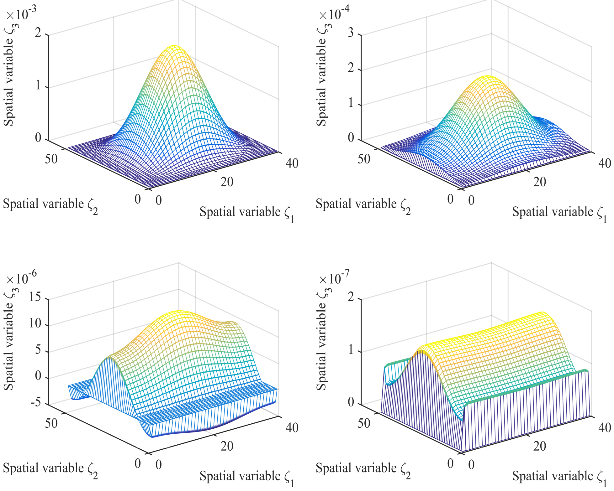
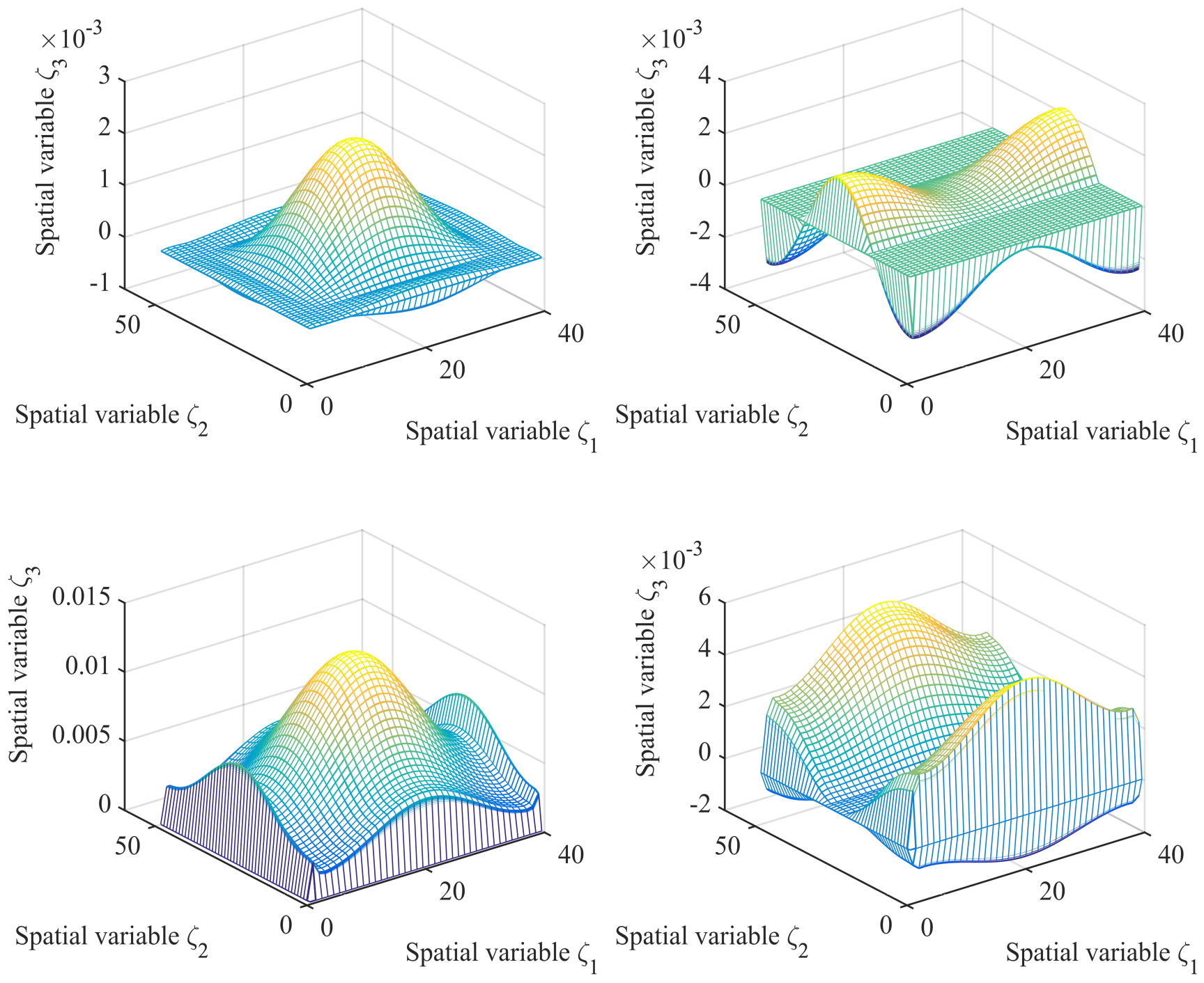
In this section, simulations are given to illustrate how these results can be applied to achieve finite-time bounded in 3D filtering error system. With Dirichlet boundary conditions, we take into consideration a class of 3D nonlinear distributed parameter systems subject to the initial condition $\eta (0,{\zeta }_1,{\zeta }_2,{\zeta }_3)={({\zeta }_1/l_1)}^3{(1-{\zeta }_1/l_1)}^3{({\zeta }_2/l_2)}^3{(1-{\zeta }_2/l_2)}^3{({\zeta }_3/l_3)}^3{(1-{\zeta }_3/l_3)}^3$, where $l_1=1,l_2=0.5,l_3=0.8$. The system parameters are proposed as follows: $a_0={10}^{-5}$ and $f(t,\eta (t,\zeta \left)\right)=\arctan \left(0.7\eta \right(t,\zeta \left)\right)$. The evolution of the 3D nonlinear distributed parameter system at four different times is shown in Figure 2.

The coordinate system in Figure 2 represents a three-dimensional space. Hence, the states of the system in three dimensions at time $t=0.25,1,2,5$ s, respectively, need to be shown using four different spatial coordinate systems.

Two mobile sensing devices are taken into account, and their initial locations are selected as $({\zeta }_{11}\left(0\right),{\zeta }_{12}\left(0\right),{\zeta }_{13}\left(0\right))=(0.18,0.10,0.25)$ and $({\zeta }_{21}\left(0\right),{\zeta }_{22}\left(0\right),$${\zeta }_{23}\left(0\right))=(0.56,0.14,0.32)$. The sensor network coupling matrix $\Pi =\left[\begin{array}{cc}-1& 1\\ 1& -1\end{array}\right]$. Their spatial distribution is defined by

$${\psi }_i({\zeta }_s;{\zeta }_{is}\left(t\right))=\left\{\begin{array}{c}1\mathrm{if}\zeta \in {\Omega }_i\hfill \\ 0\mathrm{otherwise}.\hfill \end{array}\right.$$

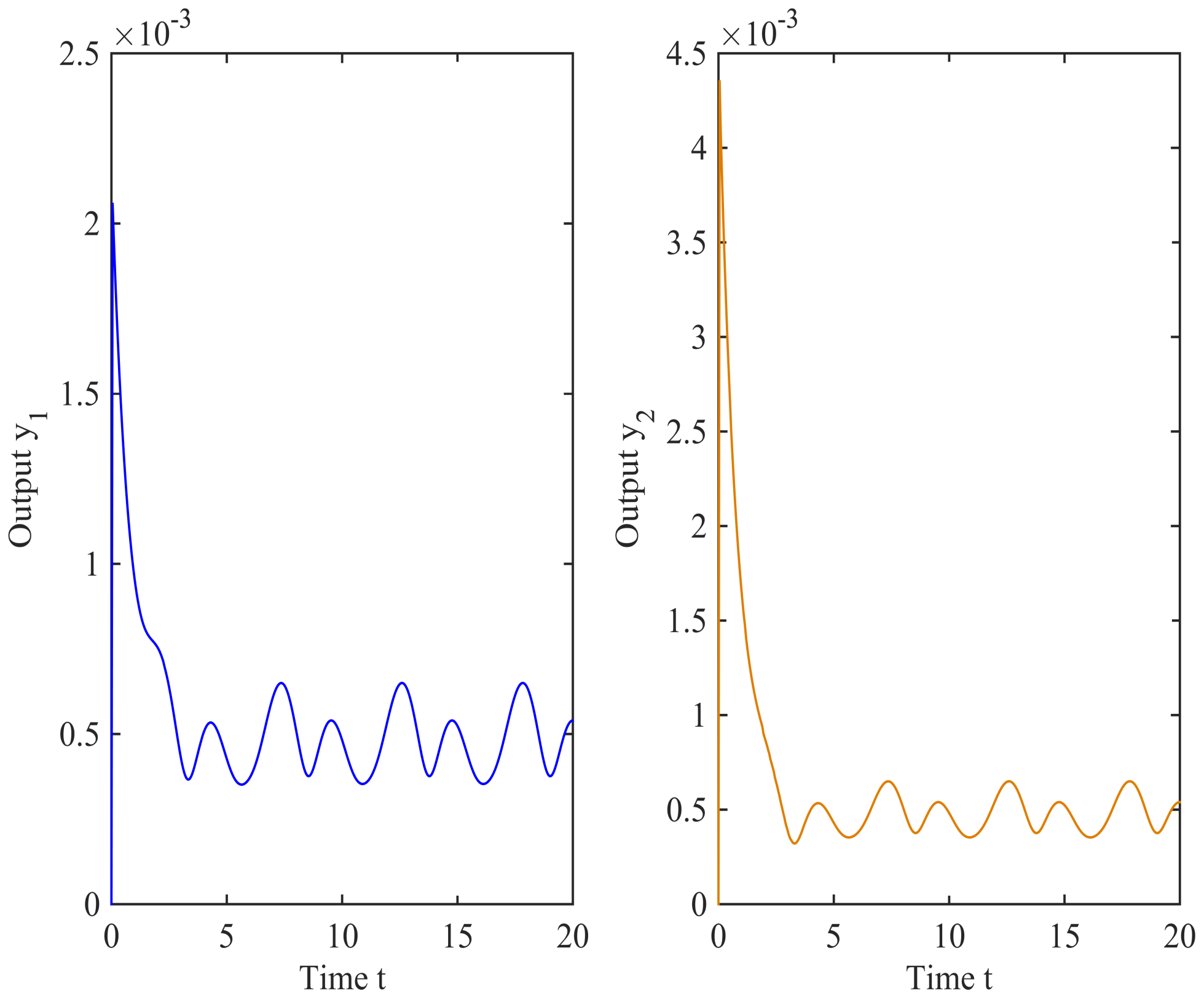
In this simulation, the probabilities are taken as $\overline{\rho }=0.75$, ${\overline{ϵ}}_1=0.9$ and ${\overline{ϵ}}_2=0.85$; the perturbation attenuation level is $\gamma =0.95$; $\sigma \left(y_i\left(t\right)\right)$ is a saturation function written in the following:

$$\sigma \left(y_i\left(t\right)\right)=\left\{\begin{array}{c}\sigma \left(y_i\left(t\right)\right)=V_{i,max},\mathrm{if}{y}_i\left(t\right)>V_{i,max}\hfill \\ \sigma \left(y_i\left(t\right)\right)=y_i\left(t\right),\mathrm{if}-V_{i,max}\le y_i\left(t\right)\le V_{i,max}\hfill \\ \sigma \left(y_i\left(t\right)\right)=-V_{i,max},\mathrm{if}{y}_i\left(t\right)<-V_{i,max}\hfill \end{array}\right.$$

The saturation values are taken as $V_1=V_2=0.07$. The measurement output of mobile sensors with randomly sensor saturation are depicted in Figure 3.

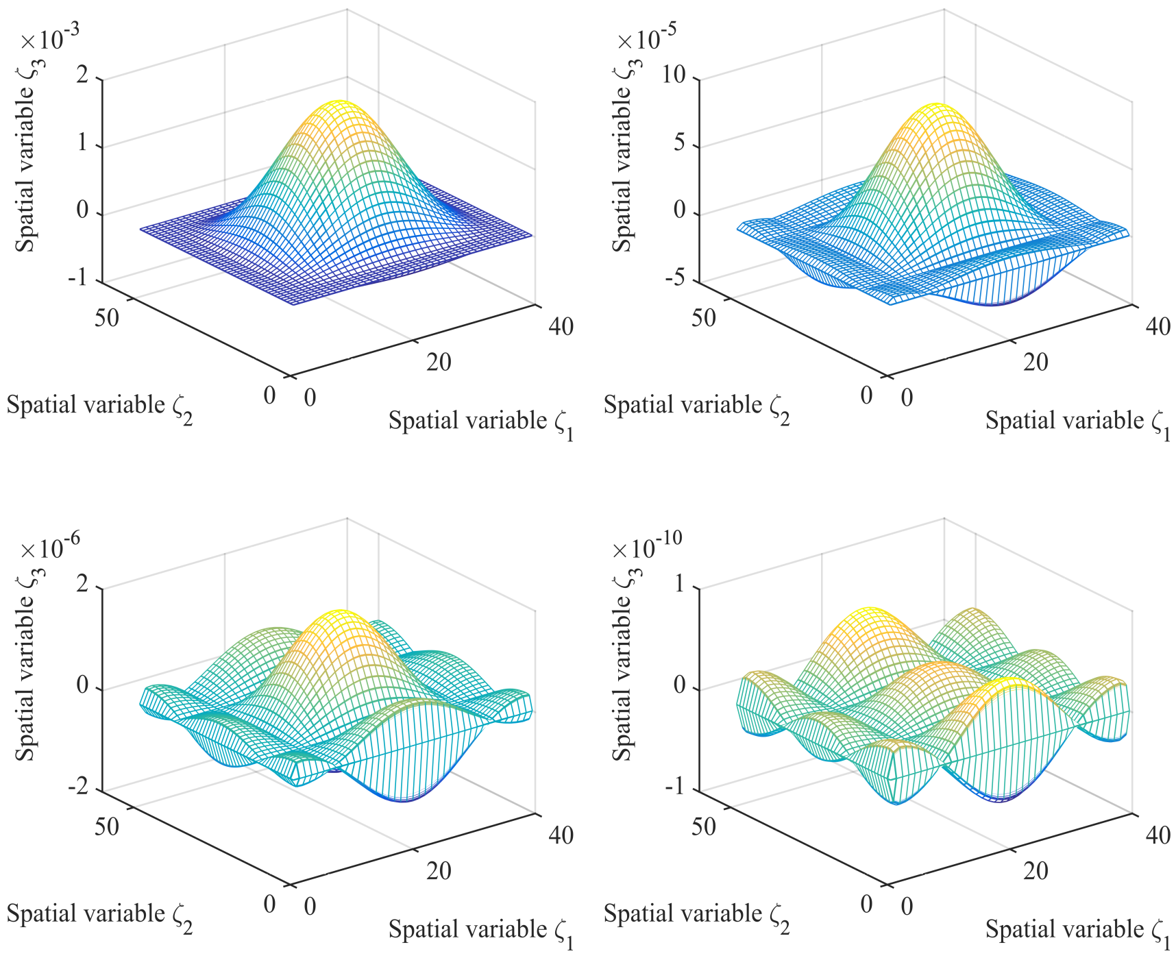
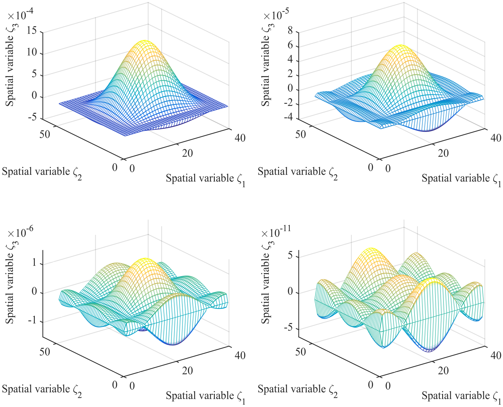
The initial condition for the distributed consensus filter is selected to be ${\widehat{\eta }}_1(0,\zeta )={\widehat{\eta }}_2(0,\zeta )=0$. Gain for the distributed filters is determined by $k_1=10$ and $k_2=30$. Figure 4 and Figure 5 illustrate how the filtering errors of the two distributed $H_{\infty }$ consensus filters changed at four different times in the first 5 s. After 5 s, with increasing time, their filtering errors converge rapidly to the bounds. Figure 6 and Figure 7 show the estimation results of the two distributed filters at four different times, respectively.

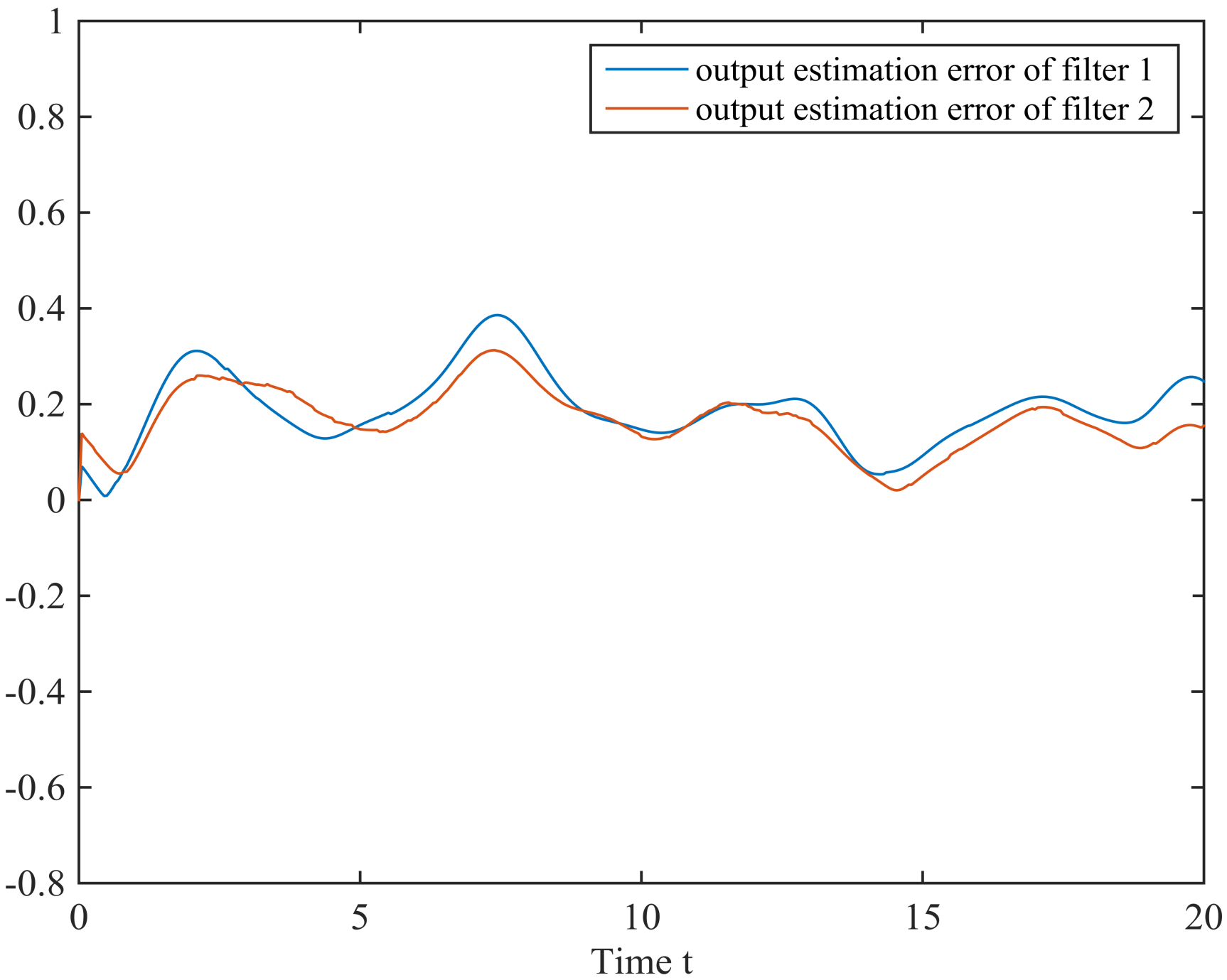
Figure 8 displays the output estimation errors for the two filters. The estimation converges to the bounded range in a short time, as can be seen in Figure 8. The existence of the estimation error is caused by the bounded perturbation in the system. Once the perturbation decays or even disappears, then the estimation error converges rapidly to zero.

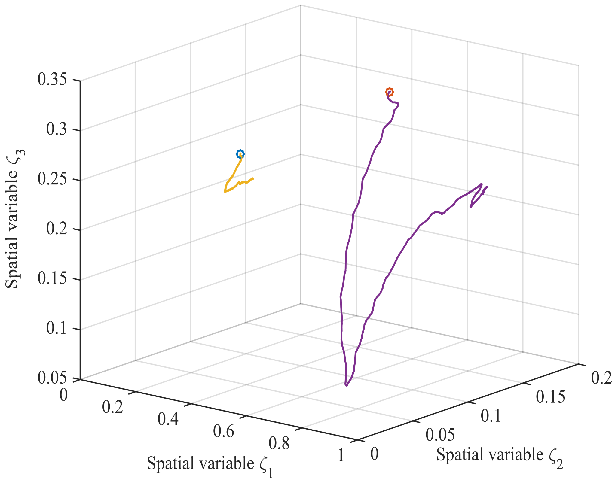
To reflect the enhanced filtering performance of the motion sensing approach, we introduce fixed sensors for comparison with mobile sensors. The two fixed sensors are located at $({\zeta }_{11},{\zeta }_{12},{\zeta }_{13})=(0.18,0.10,0.25)$ and $({\zeta }_{21},{\zeta }_{22},{\zeta }_{23})=(0.56,0.14,0.32)$.These two locations are indicated by small circles in Figure 9. These two spatial locations are also the initial locations before the mobile sensor moves. As a comparison with the fixed sensor, the trajectories of the two mobile sensors under velocity constraints are also shown in Figure 9.

In Figure 10, the effect of the evolution of the $L_2$ norm of the filtering error for the two fixed sensors and the two mobile sensors is shown. The appreciable reduction of the state norm is observed for the mobile case.

6. Conclusions

This paper has addressed the issue of finite-time distributed $H_{\infty }$ consensus filtering for a class of 3D nonlinear distributed parameter systems subject to bounded perturbation. The considered incomplete information in measured output is randomly occurring sensor saturation. Specialized conditions are used to treat the system and possible output saturation. A mobile sensing approach is proposed as a new framework for optimizing the filtering issue, thus enhancing the performance of the filter. Moreover, a novel nonlinear stochastic decomposition model is proposed. With a guaranteed $H_{\infty }$ consensus disturbance rejection attenuation level and dynamics of the filtering error system that are finite-time bounded, a novel distributed $H_{\infty }$ consensus filter has been developed. In light of the operator-dependent Lyapunov function, the finite-time bounded of the filtering error system can be achieved. For the simplified analysis, the spatial distribution of the selected mobile sensing devices is symmetric, and therefore, the closed-loop operator in the evolution equation is self-adjoint. In a more general case, the spatial distribution may not be symmetric, and even may not be derivative with respect to the location. Then the analysis of the closed-loop operator will be a challenge and is being considered by the authors. The filtering error system is able to converge faster, also dependent on conditions in the form of the velocity law for the mobile sensors. It has been demonstrated through numerical simulations that the proposed criteria are effective.