Stochastic Epidemic Model for COVID-19 Transmission under Intervention Strategies in China

Abstract

In this paper, we discuss an EIQJR model with stochastic perturbation. First, a globally positive solution of the proposed model has been discussed. In addition, the global asymptotic stability and exponential mean-square stability of the disease-free equilibrium have been proven under suitable conditions for our model. This means that the disease will die over time. We investigate the asymptotic behavior around the endemic equilibrium of the deterministic model to show when the disease will prevail. Constructing a suitable Lyapunov functional method is crucial to our investigation. Parameter estimations and numerical simulations are performed to depict the transmission process of COVID-19 pandemic in China and to support analytical results.

1. Introduction

In December 2019, the outbreak of the novel coronavirus disease 2019 (COVID-19/2019-nCoV/SARS-CoV-2) was detected in China [1,2]. The COVID-19 virus is similar to the severe acute respiratory syndrome (SARS) virus [3], but it is more contagious than SARS [4]. According to the public health community [5] and the WHO [6], close contact between infected individuals is the primary way that the COVID-19 virus spreads. The disease can be spread by respiratory droplets from coughs and sneezes of the infected individuals [7,8], and another way to get infected is by indirect contact with contaminated surfaces [9]. The essential strategies for controlling virus infection include early identification, quarantine, diagnosis, isolation, and treatment [10]. While epidemiologists have continued to do a lot of research on COVID-19 [11], mathematicians have developed and studied the mathematical models to help in the formulation of control strategies [12].

It is necessary to establish a mathematical model to estimate the dynamics of the transmission and control of the virus. Thus, a large number of scholars are concentrating on mathematical modeling [11,13,14,15,16,17]. For example, Wu et al. extended the SEIR model into SEIR meta-population model to simulate the outbreak of 2019-nCoV across all major cities in China and predicted the national and global outbreak of 2019-nCoV [17]. In [13], Lu et al. established a conceptual model for COVID-19 transmission in Wuhan, taking into account individual reactions as well as government-controlled action. Chen et al. constructed a Bats-Hosts-Reservoir-People transmission network model in order to simulate the potential transmission from the infection source (likely bats) to the human [14]. Authors have established a SEIQR model that included an isolation class in order to show the dynamic behavior of the COVID-19 infection [18]. Tang et al. developed a baseline model to reduce the transmission from the campus of a university into the wider community, or from the wider community to the campus of university [15]. Xiao et al. evaluated that a classical SIR epidemic model could be used to reduce transmission during the entire outbreak by combining the intervention options and media impacts [16]. Because the number of exposed, infected, quarantined, diagnosed, and recovered members is so small compared to susceptible individuals, Zhou and Ma assumed that the infectious members of the population are sufficient to transmit infections to susceptible individuals (the population size of China) and then produce new infections, neglecting contacts with the others [12]. As a consequence, they forecasted on exposed, infected, quarantined, diagnosed, and recovered members, and developed the discrete EIQJR model as follows:

$$\begin{array}{cc}\hfill E(t+1)& =E\left(t\right)+\beta \left(t\right)\left(kE\right(t)+I(t\left)\right)-(\epsilon +\lambda )E\left(t\right),\hfill \\ \hfill I(t+1)& =I\left(t\right)+\epsilon E\left(t\right)-(\delta +\theta )I\left(t\right),\hfill \\ \hfill Q(t+1)& =Q\left(t\right)+\lambda E\left(t\right)-\sigma Q\left(t\right),\hfill \\ \hfill J(t+1)& =J\left(t\right)+\theta I\left(t\right)+\sigma Q\left(t\right)-(\delta +\gamma )J\left(t\right),\hfill \\ \hfill R(t+1)& =R\left(t\right)+\gamma J\left(t\right).\hfill \end{array}$$

(1)

In system (1), they define the basic reproductive ratio, $R_0=\frac{{\beta }^{*}(\epsilon +k(\delta +\theta ))}{(\epsilon +\lambda )(\delta +\theta )}$, and showed that the disease-free equilibrium $P^0=(0,0,0,0,0)$ is globally asymptotically stable when $R_0<1$. However, the authors didn’t consider the effects of random perturbations of the disease spreading and intervention strategies in the previous works. Continuous approximations of discrete-time models are often used because of their mathematical tractability [19]. And infection events can take place at every point in time. Thus continuous-time analogue model with stochastic perturbation is interesting to consider in this article.

In mathematical modeling of an infectious disease, the deterministic approach has some restrictions, and it is difficult to anticipate the future dynamics of the system accurately. This occurs because deterministic models do not take the impact of a changing environment into account. In fact, the spread of disease can actually be influenced by a wide variety of random factors. For example, mobility, urban density, and population travelling may have significant effects on the spread of COVID-19. Because of a higher level of travelling, population mobility can increase the transmission rate [20]. Therefore, the effects of these random factors can be translated to the fluctuations in the transmission rate [21]. The parameters used in the modeling approach are not absolute constants, and they oscillate around some average values because of environmental fluctuations. The arguments for establishing stochastic models are the changes in our social and environmental distinctions in our daily life [22]. Therefore, many researchers have explored that introducing parameter perturbation can affect population dynamics [23,24,25,26,27,28]. For example, Ji et al. considered the fluctuations in parameter $\beta$ and examined the effect of oscillating environment on SIR system [25]. Hou et al. considered a stochastic SIHR epidemic model of COVID-19 with the effects of parameter perturbation [29]. The authors considered the fluctuations of transmission rates and proposed stochastic SIHR COVID-19 model [30]. Lahrouz et al. considered a stochastic SIRS model by perturbing the deterministic system by a white noise [28]. Ikram et al. proposed the COVID-19 SIVR model with stochastic perturbation and proved the extinction of the model and ergodic stationary distribution under suitable conditions [22]. Recently, Tesfaye and Satana proposed the stochastic COVID-19 SVITR model [31], Zhang et al. considered the dynamics of stochastic COVID-19 SIR model [32], Ding et al. formulated stochastic COVID-19 SEIR model with Lévy noise [33], Ninno–Torres et al. constructed a stochastic COVID-19 model with random perturbation [34], Tesfay et al. established stochastic COVID-19 SIR model with jump-diffusion [35]. Although several articles examine the effect of stochastic perturbation on the SIR, SIVR, and SIRS epidemic, we are unaware of any literature addressing the issue of stochastic COVID-19 EIQJR model dynamics, which reveals primarily as fluctuations in transmission coefficient $\epsilon$ and diagnosis coefficient $\sigma$. This study attempts to fill that need.

One of the main objectives of this work is to study how stochastic perturbations in the infectious and diagnosis forces affect the disease dynamics, by investigating the global asymptotic stability of disease-free equilibrium. In addition, we deduce the dynamical behavior of the solution around the endemic equilibrium of the deterministic model to investigate whether the disease would prevail. Numerical experiments are performed to depict the transmission of COVID-19 in China, to describe the impact of noises on the population and to support our theoretical results.

The paper is organized as follows. In Section 2, we formulate the stochastic EIQJR model for COVID-19 transmission. The unique global positive solution of the system is given in Section 3. We analyze the stochastically asymptotic stability in the large and exponentially mean square stability of disease-free equilibrium in Section 4. We discuss the behavior of the solution around the endemic equilibrium in Section 5. After estimating the parameters, numerical experiments are carried out to support our analytical results and to show the impact of parameters in Section 6. Conclusions are provided in Section 7.

2. EIQJR COVID-19 Model

Let $(\mathsf{\Omega },F,{\left\{F_t\right\}}_{t\ge 0},\mathbb{P})$ be a complete probability space with a filtration ${\left\{F_t\right\}}_{t\ge 0}$ satisfying the standard conditions (i.e., it is right continuous, and $F_0$ contains all P null sets) throughout this work. $a\vee b$ is used to denote $max\left\{a,b\right\}$, $a\wedge b$ is used to denote $min\left\{a,b\right\}$, and a.s. is used to mean almost surely. The indicator function of a set G will be denoted by $I_G$.

We consider the disease infection coefficient $\epsilon$ and diagnosis coefficient $\sigma$ in the model (1). This can be interpreted to mean that a potentially exposed individual will spread the disease if they come into contact with another individual, and that a potentially infectious individual will spread the disease if an infected individual comes into contact with a susceptible individual while diagnosing the quarantine individual. In the proposed model, we assume that some stochastic environmental components operate on each individual continuously over a small time interval $[t,t+dt)$, and notation $d·$ is considered for the small change in any quantity over this time interval.

In the time range $[t,t+dt)$, a single exposed individual makes $\epsilon dt$ possibly exposed contacts with each other individual, and a single infected individual makes $\sigma dt$ the potentially infectious connections with each other individual. As a result, $\epsilon$ changes to a random variable $\tilde{\epsilon }$ and $\sigma$ changes to a random variable $\tilde{\sigma }$. More exactly, each exposed individual makes $\tilde{\epsilon }dt=\epsilon dt+{\alpha }_{1}d{B}_1\left(t\right)$ possibly exposed contacts with every other individual in $[t,t+dt)$, and each infectious individual makes $\tilde{\sigma }dt=\sigma dt+{\alpha }_{2}d{B}_2\left(t\right)$ potentially infectious contacts with every other individual. By using $\tilde{\epsilon }$ and $\tilde{\sigma }$ in system (1), we can construct a new stochastic EIQJR model as follows:

$$\begin{array}{cc}\hfill dE& =[\beta \left(t\right)(kE+I)-(\epsilon +\lambda )E]dt-{\alpha }_{1}Ed{B}_1\left(t\right),\hfill \\ \hfill dI& =[\epsilon E-(\delta +\theta )I]dt+{\alpha }_{1}Ed{B}_1\left(t\right),\hfill \\ \hfill dQ& =[\lambda E-\sigma Q]dt-{\alpha }_{2}Qd{B}_2\left(t\right),\hfill \\ \hfill dJ& =[\theta I+\sigma Q-(\delta +\gamma )J]dt+{\alpha }_{2}Qd{B}_2\left(t\right),\hfill \\ \hfill dR& =\gamma Jdt,\hfill \end{array}$$

(2)

where ${\alpha }_i,i=1,2$ represents the intensity of the noise, and $d{B}_1$ and $d{B}_2$ are independent standard Brownian motions defined on a complete probability space. As pointed out in [12], $E\left(t\right)$ denotes the number of infectious individuals who are asymptomatic and possibly infectious (without infectivity or with very low infectivity) during the incubation period, $I\left(t\right)$ is the number of infected individuals who have not been quarantined, $Q\left(t\right)$ is the number of infected individuals who have been quarantined but have not been diagnosed, $J\left(t\right)$ is the number of infected individuals who have been diagnosed and quarantined, and $R\left(t\right)$ is the number of individuals who have recovered from the disease and are fully immune to reinfection. $\delta$ is the COVID-19 induced-death rate, $\gamma$ is the recovery rate, $\epsilon$ is the infection rate of exposed individuals, $\lambda$ is the quarantine rate of exposed individuals, $\sigma$ is the diagnosis rate of quarantined individuals, $\theta$ is the diagnosis rate of the infected individual, and k is the infectively proportion of exposed individuals compared to infective individuals. In [12], $\beta \left(t\right)$ is the transmission rate per day. In this study, we consider the long-term behaviors of the system (2). The transmission rate $\beta \left(t\right)$ is time-dependent and assumed to be piecewise constant, which is to indicate the dramatic changes in prevention and control policy. Thus $\beta \left(t\right)$ can be considered such as ${\beta }_0$, the minimun number of contacts per unit time due to stringent control measures and ${\beta }^{*}$, the maximum number of new infective individuals produced by a typical infective individual per unit time during the entire course of the outbreak. For simplicity of analysis, we assume that $\beta \left(t\right)={\beta }^{*}$ is constant in the remaining sections. So we will consider the stochastic EIQJR model with constant coefficients. Denote ${\mathbb{R}}_{+}^5=\left\{x\in {\mathbb{R}}^5:x_i>0,i=1,2,3,4,5\right\}$ and ${\overline{\mathbb{R}}}_{+}^5=\left\{x\in {\mathbb{R}}^5:x_i\ge 0,i=1,2,3,4,5\right\}$.

3. Global Positive Solution of Stochastic EIQJR Model

By proving the following theorem, we show the global positive solution of the proposed stochastic EIQJR COVID-19 model.

Theorem 1.

For any initial value $(E_0,I_0,Q_0,J_0,R_0)\in {\mathbb{R}}_{+}^5$, there is a unique solution $\left(E\right(t),I(t)$, $Q\left(t\right),J\left(t\right),R\left(t\right))$ of system (2) on $t\ge 0$, and the solution will remain in ${\mathbb{R}}_{+}^5$ with probability 1, namely $(E\left(t\right),I\left(t\right),Q\left(t\right),J\left(t\right),R\left(t\right))\in {\mathbb{R}}_{+}^5$ for all $t\ge 0$ almost surely.

Proof. 

Because the coefficients of the equation are locally Lipschitz continuous for any given initial value $(E\left(0\right),I\left(0\right),Q\left(0\right),J\left(0\right),R\left(0\right))\in {\mathbb{R}}_{+}^5$, there is a unique local solution

$\left(E\right(t),I(t),Q(t),J(t),R(t\left)\right)$ on $t\in [0,{\tau }_e)$, where ${\tau }_e$ is the explosion time [36].

Let $N\left(t\right)=E\left(t\right)+I\left(t\right)+Q\left(t\right)+J\left(t\right)+R\left(t\right)$, and we obtain from the system (2)

$$\begin{array}{cc}\hfill dN\left(t\right)& =[{\beta }^{*}kE+{\beta }^{*}(I+Q+J+R)-\delta (I+J)-{\beta }^{*}(Q+J+R)]dt\hfill \\ \hfill & \le [{\beta }^{*}kE+{\beta }^{*}(I+Q+J+R)]dt\hfill \end{array}$$

Since $E\left(t\right)\ge 0,I\left(t\right)\ge 0,Q\left(t\right)\ge 0,J\left(t\right)\ge 0$ and $R\left(t\right)\ge 0$ on $t\in [0,{\tau }_e)$, we have

$$\begin{array}{c}\hfill dN\left(t\right)\le CN\left(t\right)dt\end{array}$$

where $C=max\left\{{\beta }^{*}k,{\beta }^{*}\right\},k\ge 1$. Let $N_1\left(t\right)$ be the solution of the equation for any initial value $(E\left(0\right),I\left(0\right),Q\left(0\right),J\left(0\right),R\left(0\right))\in R_{+}^5$:

$$\begin{array}{cc}\hfill d{N}_1\left(t\right)& =C{N}_1\left(t\right)dt,\hfill \\ \hfill N_1\left(0\right)& =N\left(0\right),\hfill \end{array}$$

(3)

and we get

$$N_1\left(t\right)\le (E\left(0\right)+I\left(0\right)+Q\left(0\right)+J\left(0\right)+R\left(0\right))e^{Ct}:=H.$$

By differential equation comparison theorem, we get

$$N\left(t\right)\le N_1\left(t\right)\le H,$$

and $E\left(t\right)+I\left(t\right)+Q\left(t\right)+J\left(t\right)+R\left(t\right)\le H$, $t\in [0,{\tau }_e)$$a.s.$

To show this solution is global, we have to show that ${\tau }_e=\infty$, a.s. Let $k_0\ge 1$ be sufficiently large so that $E\left(0\right),I\left(0\right),Q\left(0\right),J\left(0\right)$ and $R\left(0\right)$ all lie within the interval $[\frac{1}{k_0},k_0]$, for each integer $k\ge k_0$, define the stopping time

$$\begin{array}{c}\hfill {\tau }_k=inf\left\{t\in [0,{\tau }_e):min\left\{D\left(t\right)\right\}\le \frac{1}{k}\mathrm{or}max\left\{D\left(t\right)\right\}\ge k\right\},\end{array}$$

(4)

where we let $D\left(t\right)=\left(E\right(t),I(t),Q(t),J(t),R(t\left)\right)$. Throughout this article, we set $inf\varphi =\infty$ (as usual, $\varphi$ denotes the empty set). Clearly, ${\tau }_k$ is increasing as $k\to \infty$. Set ${\tau }_{\infty }={lim}_{k\to \infty }{\tau }_k$, when ${\tau }_{\infty }\le {\tau }_e$ a.s. If we can show that ${\tau }_{\infty }=\infty$ a.s, then ${\tau }_e=\infty$ and $(E\left(t\right),I\left(t\right),Q\left(t\right),J\left(t\right),R\left(t\right))\in {\mathbb{R}}_{+}^5$ a.s for all $t\ge 0$. In other words, we need to show that ${\tau }_{\infty }=\infty$ a.s in order to complete the proof. If this assertion is false, then there is a pair of constants $T>0$ and $\eta \in (0,1)$ such that

$$\mathbb{P}\left\{{\tau }_{\infty }<T\right\}>\eta .$$

So, there is an integer $k_1\ge k_0$ such that

$$\mathbb{P}\left\{{\tau }_k\le T\right\}\ge \eta \mathrm{for}\mathrm{all}k\ge k_1.$$

(5)

Consider the function $V(E,I,Q,J,R)\in {\mathbb{R}}_{+}^5$ by

$$\begin{array}{cc}\hfill V(E,I,Q,J,R)& =(E-1-logE)+(I-1-logI)+(Q-1-logQ)\hfill \\ \hfill & +(J-1-logJ)+(R-1-logR).\hfill \end{array}$$

(6)

The nonnegativity of this function can be noticed in $(u-1-logu),\forall u>0$.

By using It$\widehat{o}$ formula, we get

$$\begin{array}{cc}\hfill dV& =(1-\frac{1}{E})[\left\{{\beta }^{*}(kE+I)-(\epsilon +\lambda )E\right\}dt-{\alpha }_{1}Ed{B}_1\left(t\right)]+\frac{{\alpha }_1^2}{2}dt\hfill \\ \hfill & +(1-\frac{1}{I})[\left\{\epsilon E-(\delta +\theta )I\right\}dt+{\alpha }_{1}Ed{B}_1\left(t\right)]+\frac{{\alpha }_1^2}{2}\frac{E^2}{I^2}dt\hfill \\ \hfill & +(1-\frac{1}{Q})[(\lambda E-\sigma Q)dt-{\alpha }_{2}Qd{B}_2\left(t\right)]+\frac{{\alpha }_2^2}{2}dt\hfill \\ \hfill & +(1-\frac{1}{J})[\left\{\theta I+\sigma Q-(\delta +\gamma )J\right\}dt+{\alpha }_{2}Qd{B}_2\left(t\right)]+\frac{{\alpha }_2^2}{2}\frac{Q^2}{J^2}dt+(1-\frac{1}{R})\left[\gamma J\right]dt\hfill \\ \hfill & =[{\beta }^{*}(kE+I)-(\epsilon +\lambda )E+\epsilon E-(\delta +\theta )I+\lambda E-\sigma Q+\theta I+\sigma Q\hfill \\ \hfill & -(\delta +\gamma )J+\gamma J+\frac{{\alpha }_1^2}{2}(1+\frac{E^2}{I^2})+\frac{{\alpha }_2^2}{2}(1+\frac{Q^2}{J^2})-{\beta }^{*}k-{\beta }^{*}\frac{I}{E}+\epsilon +\lambda \hfill \\ \hfill & -\epsilon \frac{E}{I}+\delta +\theta -\lambda \frac{E}{Q}+\sigma -\theta \frac{I}{J}-\sigma \frac{Q}{J}+\delta +\gamma -\gamma \frac{J}{R}]dt\hfill \\ \hfill & -{\alpha }_1(E-1)d{B}_1\left(t\right)+{\alpha }_1\frac{E(I-1)}{I}d{B}_1\left(t\right)-{\alpha }_2(Q-1)d{B}_2\left(t\right)\hfill \\ \hfill & +{\alpha }_2\frac{Q(J-1)}{J}d{B}_2\left(t\right)\hfill \\ \hfill & \le \mathrm{[}{\beta }^{*}(kE+I)+\epsilon +\lambda +2\delta +\theta +\sigma +\gamma +\frac{1}{2}({\alpha }_1^2+{\alpha }_2^2)+\frac{1}{2}{\alpha }_1^2\frac{E^2}{I^2}\hfill \\ \hfill & +\frac{1}{2}{\alpha }_2^2\frac{Q^2}{J^2}\mathrm{]}dt+{\alpha }_1\frac{I-E}{I}d{B}_1\left(t\right)+{\alpha }_2\frac{J-Q}{J}d{B}_2\left(t\right).\hfill \end{array}$$

$$\begin{array}{cc}\hfill dV& \le [{\beta }^{*}kH+{\beta }^{*}H+\epsilon +\lambda +2\delta +\theta +\sigma +\gamma +\frac{1}{2}({\alpha }_1^2+{\alpha }_2^2)+\frac{1}{2}{\alpha }_1^2\frac{H^2}{H^2}+\frac{1}{2}{\alpha }_2^2\frac{H^2}{H^2}]dt\hfill \\ \hfill & +{\alpha }_1\frac{I-E}{I}d{B}_1\left(t\right)+{\alpha }_2\frac{J-Q}{J}d{B}_2\left(t\right)\hfill \\ \hfill & :=\tilde{K}dt+{\alpha }_1\frac{I-E}{I}d{B}_1\left(t\right)+{\alpha }_2\frac{J-Q}{J}d{B}_2\left(t\right).\hfill \end{array}$$

where $\tilde{K}:={\beta }^{*}kH+{\beta }^{*}H+\epsilon +\lambda +2\delta +\theta +\sigma +\gamma +\frac{1}{2}({\alpha }_1^2+{\alpha }_2^2)+\frac{1}{2}{\alpha }_1^2\frac{H^2}{H^2}+\frac{1}{2}{\alpha }_2^2\frac{H^2}{H^2}$ is the positive number and therefore, if $t_1\le T$,

$$\begin{array}{cc}\hfill {\int }_0^{{\tau }_k\wedge t_1}dV(E\left(t\right),I\left(t\right),Q\left(t\right),J\left(t\right),R\left(t\right))& \le {\int }_0^{{\tau }_k\wedge t_1}\tilde{K}dt+{\int }_0^{{\tau }_k\wedge t_1}{\alpha }_1\frac{I-E}{I}d{B}_1\left(t\right)\hfill \\ \hfill & +{\int }_0^{{\tau }_k\wedge t_1}{\alpha }_2\frac{J-Q}{J}d{B}_2\left(t\right).\hfill \end{array}$$

This means that,

$$\begin{array}{cc}\hfill \mathbb{E}[& V(E({\tau }_k\wedge t_1),I({\tau }_k\wedge t_1),Q({\tau }_k\wedge t_1),J({\tau }_k\wedge t_1),R({\tau }_k\wedge t_1))]\hfill \\ \hfill & \le V(E_0,I_0,Q_0,J_0,R_0)+\mathbb{E}{\int }_0^{{\tau }_k\wedge t_1}\tilde{K}dt\hfill \\ \hfill & =V(E_0,I_0,Q_0,J_0,R_0)+\tilde{K}\mathbb{E}({\tau }_k\wedge t_1)\le V(E_0,I_0,Q_0,J_0,R_0)+\tilde{K}T.\hfill \end{array}$$

(7)

Set ${\mathsf{\Omega }}_k=\left\{{\tau }_k\le T\right\}$ and by (5), $\mathbb{P}\left({\mathsf{\Omega }}_k\right)\ge \eta$. Note that, for every $\omega \in {\mathsf{\Omega }}_k$, there is at least one of $E({\tau }_k,\omega ),I({\tau }_k,\omega ),Q({\tau }_k,\omega ),J({\tau }_k,\omega )$ and $R({\tau }_k,\omega )$ which are equal to either k or $\frac{1}{k}$, then $V(E({\tau }_k,\omega ),I({\tau }_k,\omega ),Q({\tau }_k,\omega ),J({\tau }_k,\omega ),R({\tau }_k,\omega ))$ is no less than

$$k-1-logk\mathrm{or}\frac{1}{k}-1-log\frac{1}{k}=\frac{1}{k}-1+logk.$$

Hence,

$$V(E({\tau }_k,\omega ),I({\tau }_k,\omega ),Q({\tau }_k,\omega ),J({\tau }_k,\omega ),R({\tau }_k,\omega ))\ge (k-1-logk)\wedge (\frac{1}{k}-1+logk).$$

It follows from (5) and (7) that

$$\begin{array}{cc}\hfill V(E_0,I_0,Q_0,J_0,R_0)+\tilde{K}T& \ge \mathbb{E}\left[1_{{\mathsf{\Omega }}_k\left(\omega \right)}V(E({\tau }_k,\omega ),I({\tau }_k,\omega ),Q({\tau }_k,\omega ),J({\tau }_k,\omega ),R({\tau }_k,\omega ))\right]\hfill \\ \hfill & \ge \eta [(k-1-logk)\wedge (\frac{1}{k}-1+logk)],\hfill \end{array}$$

(8)

where $1_{{\mathsf{\Omega }}_k\left(\omega \right)}$ is the indicator function of ${\mathsf{\Omega }}_k$. Letting $k\to \infty$ we obtain the contradiction $\infty >V(E_0,I_0,Q_0,J_0,R_0)+\tilde{K}T=\infty$. So we must have ${\tau }_{\infty }=\infty$ a.s. The proof is complete. □

Remark 1.

For any initial value $(E_0,I_0,Q_0,J_0,R_0)\in {\mathbb{R}}_{+}^5$, we have $E\left(t\right)+I\left(t\right)+Q\left(t\right)+J\left(t\right)+R\left(t\right)\le (E\left(0\right)+I\left(0\right)+Q\left(0\right)+J\left(0\right)+R\left(0\right))e^{Ct}:=H$, $N\left(0\right)=E\left(0\right)+I\left(0\right)+Q\left(0\right)+J\left(0\right)+R\left(0\right)$.

4. Asymptotic Behavior of the Disease-Free Equilibrium

It is obvious that the disease-free equilibrium $P^0=(0,0,0,0,0)$ is a solution of (2). The stability of the disease-free equilibrium will be investigated to see whether it contributes to the threshold condition for managing infectious disease or elimination. The disease will eventually die out if $P^0$ is global asymptotic stable. We begin by recalling the definitions and lemmas of stochastic stability, given in [37]. Consider the general d-dimensional stochastic differential equation as follows:

$$dx\left(t\right)=f(x\left(t\right),t)dt+g(x\left(t\right),t)dB\left(t\right)\mathrm{on}t\ge t_0,$$

(9)

with initial value $x\left(t_0\right)=x_0\in {\mathbb{R}}^d$. $B\left(t\right)$ denotes d-dimensional standard Brownian motion defined on the above probability space. Assume $f(0,t)=0$ and $g(0,t)=0$ for all $t\ge t_0$. So the trivial solution $x\left(t\right)=0$ is a solution to Equation (9). Denote by $C^{2,1}({\mathbb{R}}^d\times [t_0,\infty );{\mathbb{R}}_{+})$ the family of all non-negative functions $V(x,t)$ defined on ${\mathbb{R}}^d\times [t_0,\infty )$, such that they are continuously twice differentiable in x and the first order in t. Define the differential operator L associated with Equation (9) by

$$L=\frac{\partial }{\partial t}+\sum _{i=1}^d{f}_i(x,t)\frac{\partial }{\partial x_i}+\frac{1}{2}\sum _{i,j=1}^d{\left[g^T(x,t)g(x,t)\right]}_{ij}\frac{{\partial }^2}{\partial x_i\partial x_j}.$$

If L acts on a function $V\in C^{2,1}({\mathbb{R}}^d\times [t_0,\infty );{\mathbb{R}}_{+})$, then

$$LV(x,t)=V_t(x,t)+V_x(x,t)f(x,t)+\frac{1}{2}\mathrm{trace}\left[g^T(x,t)V_{xx}(x,t)g(x,t)\right],$$

where $V_t=\frac{\partial V}{\partial t},V_x=(\frac{\partial V}{\partial x_1},\dots ,\frac{\partial V}{\partial x_d})$ and $V_{xx}={\left(\frac{{\partial }^{2}V}{\partial x_i\partial x_j}\right)}_{d\times d}.$ By It$\widehat{o}$ formula,

$$dV(x\left(t\right),t)=LV(x\left(t\right),t)dt+V_x(x\left(t\right),t)g(x\left(t\right),t)dB\left(t\right).$$

Lemma 1

([25,37]). If there exists a positive-definite decrescent radially unbounded function $V(x,t)\in C^{2,1}({\mathbb{R}}^d\times [t_0,\infty );{\mathbb{R}}_{+})$ such that $LV(x,t)$ is negative-definite, then the trivial solution of Equation (9) is stochastically asymptotically stable in the large.

Lemma 2

([25,37]). Assume that there is a function $V(x,t)\in C^{2,1}({\mathbb{R}}^d\times [t_0,\infty );{\mathbb{R}}_{+})$ and positive constants $a_1,a_2$ and $a_3$ such that

$$a_1{\left|x\right|}^p\le V(x,t)\le a_2{\left|x\right|}^{p}andLV(x,t)\le -a_{3}V(x,t),$$

for all $(x,t)\in {\mathbb{R}}^d\times [t_0,\infty )$. Then the trivial solution of (9) is exponentially mean square stable and the equilibrium $X=0$ is globally asymptotically stable.

Theorem 2.

If $R_0\le 1$ and the conditions $\epsilon +\lambda -{\beta }^{*}k-{\alpha }_1^2>0$, $\sigma >\frac{3}{2}{\alpha }_2^2$ hold, then the solution $P^0(0,0,0,0,0)$ of system (2) is stochastically asymptotically stable in the large.

Proof. 

Considering the Lyapunov function:

$$V(E,I,Q,J,R)=\frac{1}{2}{E}^2+\frac{1}{2}{I}^2+\frac{1}{2}{Q}^2+{\lambda }_1{J}^2+{(J+R)}^2,$$

where ${\lambda }_1$ is real positive constant. Because

$$\begin{array}{cc}\hfill \frac{1}{2}{E}^2+\frac{1}{2}{I}^2+\frac{1}{2}{Q}^2+{\lambda }_1{J}^2& +{(J+R)}^2=\frac{1}{2}{E}^2+\frac{1}{2}{I}^2+\frac{1}{2}{Q}^2+{\lambda }_1{J}^2+J^2\hfill \\ \hfill & +R^2+2JR\hfill \\ \hfill & \le \frac{1}{2}{E}^2+\frac{1}{2}{I}^2+\frac{1}{2}{Q}^2+({\lambda }_1+2)J^2+2R^2\hfill \end{array}$$

(10)

and

$$\begin{array}{cc}\hfill \frac{1}{2}{E}^2& +\frac{1}{2}{I}^2+\frac{1}{2}{Q}^2+{\lambda }_1{J}^2+{(J+R)}^2=\frac{1}{2}{E}^2+\frac{1}{2}{I}^2+\frac{1}{2}{Q}^2+{\lambda }_1{J}^2+J^2\hfill \\ \hfill & +R^2+2JR\hfill \\ \hfill & =\frac{1}{2}{E}^2+\frac{1}{2}{I}^2+\frac{1}{2}{Q}^2+({\lambda }_1+1)J^2+R^2+2\left(\sqrt{\frac{{\lambda }_1}{2}+1}J\right)\left(\frac{1}{\sqrt{\frac{{\lambda }_1}{2}+1}}R\right)\hfill \\ \hfill & \ge \frac{1}{2}{E}^2+\frac{1}{2}{I}^2+\frac{1}{2}{Q}^2+({\lambda }_1+1)J^2+R^2-(\frac{{\lambda }_1}{2}+1)J^2-\frac{2}{{\lambda }_1+2}{R}^2\hfill \\ \hfill & =\frac{1}{2}{E}^2+\frac{1}{2}{I}^2+\frac{1}{2}{Q}^2+\frac{{\lambda }_1}{2}{J}^2+\frac{{\lambda }_1}{{\lambda }_1+2}{R}^2.\hfill \end{array}$$

(11)

$$\begin{array}{cc}\hfill LV& =E[{\beta }^{*}(kE+I)-(\epsilon +\lambda )E]+\frac{1}{2}{\alpha }_1^2{E}^2+I[\epsilon E-(\delta +\theta )I]+\frac{1}{2}{\alpha }_1^2{E}^2\hfill \\ \hfill & +Q[\lambda E-\sigma Q]+\frac{1}{2}{\alpha }_2^2{Q}^2+2{\lambda }_{1}J[\theta I+\sigma Q-(\delta +\gamma )J]+{\lambda }_1{\alpha }_2^2{Q}^2\hfill \\ \hfill & +2(J+R)[\theta I+\sigma Q-\delta J]+{\alpha }_2^2{Q}^2\hfill \\ \hfill & ={\beta }^{*}k{E}^2-(\epsilon +\lambda )E^2+{\beta }^{*}EI+\epsilon IE-(\delta +\theta )I^2+{\alpha }_1^2{E}^2+\lambda QE\hfill \\ \hfill & -\sigma Q^2+2{\lambda }_1\theta JI+2{\lambda }_1\sigma JQ-2{\lambda }_1(\delta +\gamma )J^2+(\frac{3}{2}+{\lambda }_1){\alpha }_2^2{Q}^2\hfill \\ \hfill & +2\theta JI+2\sigma JQ-2\delta J^2+2\theta RI+2\sigma RQ-2\delta RJ.\hfill \end{array}$$

This can be simplified to

$$\begin{array}{cc}\hfill LV& =-[\epsilon +\lambda -{\beta }^{*}k-{\alpha }_1^2]E^2-[\delta +\theta ]I^2-[\sigma -(\frac{3}{2}+{\lambda }_1){\alpha }_2^2]Q^2\hfill \\ \hfill & -[2{\lambda }_1(\delta +\gamma )+2\delta ]J^2+{\beta }^{*}EI+\epsilon IE+\lambda QE+2{\lambda }_1\theta JI\hfill \\ \hfill & +2{\lambda }_1\sigma JQ+2\theta JI+2\sigma JQ+2\theta RI+2\sigma RQ-2\delta RJ.\hfill \end{array}$$

(12)

From Young’s inequality, i.e., $xy\le \frac{x^p}{p}+\frac{y^q}{q}$ for $x,y>0$ such that $p,q>0$ and $\frac{1}{p}+\frac{1}{q}=1$, and we get the following inequalities

$$\begin{array}{cccc}\hfill EI\le & \frac{1}{2}\nu E^2+\frac{1}{2\nu }{I}^2,\hfill & \hfill RQ\le & \frac{1}{2}\nu R^2+\frac{1}{2\nu }{Q}^2,\hfill \\ \hfill QE\le & \frac{1}{2\nu }{Q}^2+\frac{1}{2}\nu E^2,\hfill & \hfill RI\le & \frac{1}{2}\nu R^2+\frac{1}{2\nu }{I}^2,\hfill \\ \hfill JI\le & \frac{1}{2}\nu J^2+\frac{1}{2\nu }{I}^2,\hfill \\ \hfill JQ\le & \frac{1}{2\nu }{Q}^2+\frac{1}{2}\nu J^2.\hfill \end{array}$$

Introduce these inequalities into Equation (12), and we obtain

$$\begin{array}{cc}\hfill LV& \le -[(\epsilon +\lambda -{\beta }^{*}k-{\alpha }_1^2)-\nu (\frac{\epsilon }{2}+\frac{{\beta }^{*}}{2}+\frac{\lambda }{2})]E^2-[\delta +\theta -\frac{{\beta }^{*}}{2\nu }]I^2\hfill \\ \hfill & -[\frac{\epsilon }{2\nu }+\frac{{\lambda }_1\theta }{\nu }+\frac{2\theta }{\nu }]I^2-[\sigma -(\frac{3}{2}+{\lambda }_1){\alpha }_2^2]Q^2\hfill \\ \hfill & -[\frac{\lambda }{2\nu }+\frac{{\lambda }_1\sigma }{\nu }+\frac{2\sigma }{\nu }]Q^2-[2{\lambda }_1(\delta +\gamma )+3\delta -\nu ({\lambda }_1\theta +{\lambda }_1\sigma +\theta +\sigma )]J^2\hfill \\ \hfill & -[\delta -\nu (\theta +\sigma )]R^2.\hfill \end{array}$$

(13)

Choose $\nu$ to be sufficiently small such that the coefficients of $E^2,I^2$, and $J^2$ are negative and as $\epsilon +\lambda >{\beta }^{*}k+{\alpha }_1^2$, $\delta +\theta >{\beta }^{*}$ and $\sigma >(\frac{3}{2}+{\lambda }_1){\alpha }_2^2$, we can choose ${\lambda }_1$ to be positive such as the coefficients of $I^2,Q^2$ and $J^2$ be negative. According to Lemma 1, we conclude that the trivial solution $P^0(0,0,0,0,0)$ of system (2) is asymptotically stable in the large. □

Theorem 3.

If $R_0\le 1$ and the conditions $\epsilon +\lambda -{\beta }^{*}k-{\alpha }_1^2>0$, $\sigma >\frac{3}{2}{\alpha }_2^2$ hold, then the solution $P^0=(0,0,0,0,0)$ of system (2) is exponentially mean-square stable.

Proof. 

As in the proof of Theorem 2, we also choose the Lyapunov function:

$$V(E,I,Q,J,R)=\frac{1}{2}{E}^2+\frac{1}{2}{I}^2+\frac{1}{2}{Q}^2+{\lambda }_1{J}^2+{(J+R)}^2,$$

where ${\lambda }_1$ is a positive as in Theorem 2, and from the proof of Theorem 2, we see

$$\begin{array}{cc}\hfill V(E,I,Q,J,R)& \ge \frac{1}{2}{E}^2+\frac{1}{2}{I}^2+\frac{1}{2}{Q}^2+\frac{{\lambda }_1}{2}{J}^2+\frac{{\lambda }_1}{{\lambda }_1+2}{R}^2\hfill \\ & \ge \frac{{\lambda }_1}{{\lambda }_1+2}(E^2+I^2+Q^2+J^2+R^2)\hfill \end{array}$$

and

$$\begin{array}{cc}\hfill V(E,I,Q,J,R)& \le \frac{1}{2}{E}^2+\frac{1}{2}{I}^2+\frac{1}{2}{Q}^2+({\lambda }_1+2)J^2+2R^2\hfill \\ & \le ({\lambda }_1+2)(E^2+I^2+Q^2+J^2+R^2),\hfill \end{array}$$

that is

$$\begin{array}{cc}\hfill \frac{{\lambda }_1}{{\lambda }_1+2}(E^2+I^2+Q^2+J^2+R^2)& \le V(E,I,Q,J,R)\hfill \\ \hfill & \le ({\lambda }_1+2)(E^2+I^2+Q^2+J^2+R^2).\hfill \end{array}$$

(14)

Besides, (13) implies that

$$\begin{array}{cc}\hfill LV& \le -[\epsilon +\lambda -{\beta }^{*}k-{\alpha }_1^2]E^2-[\delta +\theta -\frac{{\beta }^{*}}{2\nu }]I^2-[\sigma -(\frac{3}{2}+{\lambda }_1){\alpha }_2^2]Q^2\hfill \\ \hfill & -[2{\lambda }_1(\delta +\gamma )+3\delta ]J^2-\delta R^2\hfill \\ \hfill & \le -min\left\{\epsilon +\lambda -{\beta }^{*}k-{\alpha }_1^2,\delta +\theta -\frac{{\beta }^{*}}{2\nu },\sigma -(\frac{3}{2}+{\lambda }_1){\alpha }_2^2,2{\lambda }_1(\delta +\gamma )+3\delta ,\delta \right\}\hfill \\ & (E^2+I^2+Q^2+J^2+R^2)\hfill \end{array}$$

$$LV\le -\frac{D}{{\lambda }_1+2}V(E,I,Q,J,R),$$

(15)

where $D=min\left\{\epsilon +\lambda -{\beta }^{*}k-{\alpha }_1^2,\delta +\theta -\frac{{\beta }^{*}}{2\nu },\sigma -(\frac{3}{2}+{\lambda }_1){\alpha }_2^2,2{\lambda }_1(\delta +\gamma )+3\delta ,\delta \right\}$.

Therefore from (14) and (15) and Lemma 2, we conclude that the trivial solution of system (2) is exponentially mean-square stable. That is to say the disease-free equilibrium $P^0=(0,0,0,0,0)$ of system (2) is exponentially mean-square stable. □

Remark 2.

Zhou and Ma [12] used discrete states representing numbers of individuals to give EIQJR model and showed the disease-free equilibrium $P^0$ is globally asymptotically stable when $R_0=\frac{{\beta }^{*}(\epsilon +k(\delta +\theta ))}{(\epsilon +\lambda )(\delta +\theta )}<1$ (cf. Theorem 2). The asymptotic behavior around $P^0$ is measured by the intensity of the noise in this continuous COVID-19 model with stochastic perturbation.

5. Asymptotic Behavior around the Endemic Equilibrium

In this section, we assume $R_0>1$ and examine the asymptotic behavior of the solution near the endemic equilibrium of the deterministic model to show when the disease will prevail.

Theorem 4.

If $R_0>1$ and the conditions $\epsilon +\lambda >{\alpha }_1^2+{\beta }^{*}k$, $\sigma >{\alpha }_2^2$ are satisfied, then for any given initial value $(E\left(0\right),I\left(0\right),Q\left(0\right),J\left(0\right),R\left(0\right))\in R_{+}^5$, the solution of model (2) has the property

$$\begin{array}{cc}\hfill \underset{t\to \infty }{lim\; sup}\frac{1}{t}& {\int }_0^t[{(E\left(u\right)-A{E}^{*})}^2+{(I-I^{*})}^2+{(Q-B{Q}^{*})}^2+{(J-J^{*})}^2+{(R-R^{*})}^2]du\hfill \\ \hfill & \le \frac{K}{N}\hfill \end{array}$$

(16)

where $A:=\frac{2(\epsilon +\lambda -{\beta }^{*}k)-\frac{{\beta }^{*}+\epsilon +\lambda }{c}}{2(\epsilon +\lambda -{\beta }^{*}k-{\alpha }_1^2)-\frac{{\beta }^{*}+\epsilon +\lambda }{c}},B:=\frac{2\sigma -(\lambda +2\sigma )c}{2(\sigma -{\alpha }_2^2)-(\lambda +2\sigma )c}$ and

$$K:=\frac{(2(\epsilon +\lambda -{\beta }^{*}k)-\frac{{\beta }^{*}+\epsilon +\lambda }{c})2{\alpha }_1^2}{2(\epsilon +\lambda -{\beta }^{*}k-{\alpha }_1^2)-\frac{{\beta }^{*}+\epsilon +\lambda }{c}}{\left(E^{*}\right)}^2+\frac{(2\sigma -(\lambda +2\sigma )c)2{\alpha }_2^2}{2(\sigma -{\alpha }_2^2)-(\lambda +2\sigma )c}{\left(Q^{*}\right)}^2,$$

$N:=min\left\{X_1,X_2,X_3,X_4,X_5\right\}$, where $X_1=2(\epsilon +\lambda -{\beta }^{*}k-{\alpha }_1^2)-\frac{{\beta }^{*}+\epsilon +\lambda }{c}$, $X_2=2(\delta +\theta )-({\beta }^{*}+\epsilon +2\theta )c$, $X_3=2(\sigma -{\alpha }_2^2)-(\lambda +2\sigma )c$, $X_4=2\delta +\gamma -\frac{\theta +\sigma }{c}$, $X_5=\frac{\delta }{2}-\frac{\theta +\sigma }{c},$ and c is a positive constant chosen sufficiently small such that $X_1>0,X_2>0,X_3>0,X_4>0,X_5>0$.

Proof. 

Define a $C^2-$ function $V:R_{+}^5\to R_{+}$ by

$$V={(E-E^{*})}^2+{(I-I^{*})}^2+{(Q-Q^{*})}^2+\frac{1}{2}{(J-J^{*})}^2+\frac{1}{2}{(J-J^{*}+R-R^{*})}^2,$$

$$\begin{array}{cc}\hfill dV& =LVdt-2(E-E^{*}){\alpha }_{1}Ed{B}_1\left(t\right)+2(I-I^{*}){\alpha }_{1}Ed{B}_1\left(t\right)-2(Q-Q^{*}){\alpha }_{2}Qd{B}_2\left(t\right)\hfill \\ \hfill & +(J-J^{*}){\alpha }_{2}Qd{B}_2\left(t\right)+(J-J^{*}+R-R^{*}){\alpha }_{2}Qd{B}_2\left(t\right),\hfill \end{array}$$

(17)

where

$$\begin{array}{cc}\hfill LV& =2(E-E^{*})[{\beta }^{*}kE+{\beta }^{*}I-(\epsilon +\lambda )E]+{\alpha }_1^2{E}^2+2(I-I^{*})[\epsilon E-(\delta +\theta )I]+{\alpha }_1^2{E}^2\hfill \\ \hfill & +2(Q-Q^{*})[\lambda E-\sigma Q]+{\alpha }_2^2{Q}^2+(J-J^{*})[\theta I+\sigma Q-(\delta +\gamma )J]+\frac{1}{2}{\alpha }_2^2{Q}^2\hfill \\ \hfill & +(J-J^{*}+R-R^{*})[\theta I+\sigma Q-\delta J]+\frac{1}{2}{\alpha }_2^2{Q}^2\hfill \\ \hfill & =2(E-E^{*})[({\beta }^{*}k-\epsilon -\lambda )(E-E^{*})+{\beta }^{*}(I-I^{*})]+2{\alpha }_1^2{E}^2\hfill \\ \hfill & +2(I-I^{*})[\epsilon (E-E^{*})-(\delta +\theta )(I-I^{*})]+2(Q-Q^{*})[\lambda (E-E^{*})-\sigma (Q-Q^{*})]\hfill \\ \hfill & +2{\alpha }_2^2{Q}^2+(J-J^{*})[\theta (I-I^{*})+\sigma (Q-Q^{*})-(\delta +\gamma )(J-J^{*})]\hfill \\ \hfill & +(J-J^{*}+R-R^{*})[\theta (I-I^{*})+\sigma (Q-Q^{*})-\delta (J-J^{*})]\hfill \\ \hfill & =-2(\epsilon +\lambda -{\beta }^{*}k){(E-E^{*})}^2+2{\alpha }_1^2{E}^2-2(\delta +\theta ){(I-I^{*})}^2\hfill \\ \hfill & +2({\beta }^{*}+\epsilon )(E-E^{*})(I-I^{*})-2\sigma {(Q-Q^{*})}^2+2\lambda (E-E^{*})(Q-Q^{*})\hfill \\ \hfill & +2{\alpha }_2^2{Q}^2+2\theta (I-I^{*})(J-J^{*})+2\sigma (Q-Q^{*})(J-J^{*})-(2\delta +\gamma ){(J-J^{*})}^2\hfill \\ \hfill & +\theta (I-I^{*})(R-R^{*})+\sigma (Q-Q^{*})(R-R^{*})-\delta (J-J^{*})(R-R^{*}).\hfill \end{array}$$

(18)

By the Young’s inequality, we get the following inequalities

$$\begin{array}{cc}\hfill & 2({\beta }^{*}+\epsilon )(E-E^{*})(I-I^{*})\le \frac{{\beta }^{*}+\epsilon }{c}{(E-E^{*})}^2+({\beta }^{*}+\epsilon )c{(I-I^{*})}^2,\hfill \\ \hfill & 2\lambda (E-E^{*})(Q-Q^{*})\le \frac{\lambda }{c}{(E-E^{*})}^2+\lambda c{(Q-Q^{*})}^2,\hfill \\ \hfill & 2\theta (I-I^{*})(J-J^{*})\le \frac{\theta }{c}{(J-J^{*})}^2+\theta c{(I-I^{*})}^2,\hfill \\ \hfill & 2\sigma (Q-Q^{*})(J-J^{*})\le \frac{\sigma }{c}{(J-J^{*})}^2+\sigma c{(Q-Q^{*})}^2,\hfill \\ \hfill & \theta (I-I^{*})(R-R^{*})\le \frac{\theta }{c}{(R-R^{*})}^2+\theta c{(I-I^{*})}^2,\hfill \\ \hfill & \sigma (Q-Q^{*})(R-R^{*})\le \frac{\sigma }{c}{(R-R^{*})}^2+\sigma c{(Q-Q^{*})}^2,\hfill \end{array}$$

where c is a positive constant to be determined later. Insert these inequalities into the Equation (18), we get

$$\begin{array}{cc}\hfill LV& \le -[2(\epsilon +\lambda -{\beta }^{*}k)-\frac{{\beta }^{*}+\epsilon +\lambda }{c}]{(E-E^{*})}^2-2{\alpha }_1^2{E}^2\hfill \\ \hfill & -[2(\delta +\theta )-({\beta }^{*}+\epsilon +2\theta )c]{(I-I^{*})}^2-[2\sigma -(\lambda +2\sigma )c]{(Q-Q^{*})}^2-2{\alpha }_2^2{Q}^2\hfill \\ \hfill & -[2\delta +\gamma -\frac{\theta +\sigma }{c}]{(J-J^{*})}^2-[\frac{\delta }{2}-\frac{\theta +\sigma }{c}]{(R-R^{*})}^2\hfill \\ \hfill & =-[2(\epsilon +\lambda -{\beta }^{*}k-{\alpha }_1^2)-\frac{{\beta }^{*}+\epsilon +\lambda }{c}]E^2+2[2(\epsilon +\lambda -{\beta }^{*}k)-\frac{{\beta }^{*}+\epsilon +\lambda }{c}]E{E}^{*}\hfill \\ \hfill & -[2(\epsilon +\lambda -{\beta }^{*}k)-\frac{{\beta }^{*}+\epsilon +\lambda }{c}]{\left(E^{*}\right)}^2-[2(\delta +\theta )-({\beta }^{*}+\epsilon +2\theta )c]{(I-I^{*})}^2\hfill \\ \hfill & -[2(\sigma -{\alpha }_2^2)-(\lambda +2\sigma )c]Q^2+2[2\sigma -(\lambda +2\sigma )c]Q{Q}^{*}-[2\sigma -(\lambda +2\sigma )c]{\left(Q^{*}\right)}^2\hfill \\ \hfill & -[2\delta +\gamma -\frac{\theta +\sigma }{c}]{(J-J^{*})}^2-[\frac{\delta }{2}-\frac{\theta +\sigma }{c}]{(R-R^{*})}^2\hfill \end{array}$$

(19)

$$\begin{array}{cc}\hfill & =-[2(\epsilon +\lambda -{\beta }^{*}k-{\alpha }_1^2)-\frac{{\beta }^{*}+\epsilon +\lambda }{c}]{(E-\frac{2(\epsilon +\lambda -{\beta }^{*}k)-\frac{{\beta }^{*}+\epsilon +\lambda }{c}}{2(\epsilon +\lambda -{\beta }^{*}k-{\alpha }_1^2)-\frac{{\beta }^{*}+\epsilon +\lambda }{c}}{E}^{*})}^2\hfill \\ \hfill & -[2(\delta +\theta )-({\beta }^{*}+\epsilon +2\theta )c]{(I-I^{*})}^2\hfill \\ \hfill & -[2(\sigma -{\alpha }_2^2)-(\lambda +2\sigma )c]{(Q-\frac{2\sigma -(\lambda +2\sigma )c}{2(\sigma -{\alpha }_2^2)-(\lambda +2\sigma )c}{Q}^{*})}^2\hfill \\ \hfill & -[2\delta +\gamma -\frac{\theta +\sigma }{c}]{(J-J^{*})}^2-[\frac{\delta }{2}-\frac{\theta +\sigma }{c}]{(R-R^{*})}^2+\frac{(2\sigma -(\lambda +2\sigma )c)2{\alpha }_2^2}{2(\sigma -{\alpha }_2^2)-(\lambda +2\sigma )c}{\left(Q^{*}\right)}^2\hfill \\ \hfill & +\frac{(2(\epsilon +\lambda -{\beta }^{*}k)-\frac{{\beta }^{*}+\epsilon +\lambda }{c})2{\alpha }_1^2}{2(\epsilon +\lambda -{\beta }^{*}k-{\alpha }_1^2)-\frac{{\beta }^{*}+\epsilon +\lambda }{c}}{\left(E^{*}\right)}^2.\hfill \end{array}$$

(20)

Besides $\epsilon +\lambda >{\alpha }_1^2+{\beta }^{*}k$, $\delta +\theta >0$, $\sigma >{\alpha }_2^2$, and we choose that c is positive and sufficiently small such that $2(\epsilon +\lambda -{\beta }^{*}k-{\alpha }_1^2)-\frac{{\beta }^{*}+\epsilon +\lambda }{c}>0$, $2(\delta +\theta )-({\beta }^{*}+\epsilon +2\theta )c>0$, $2(\sigma -{\alpha }_2^2)-(\lambda +2\sigma )c>0$, $2\delta +\gamma -\frac{\theta +\sigma }{c}>0$, $\frac{\delta }{2}-\frac{\theta +\sigma }{c}>0$.

Thus

$$\begin{array}{cc}\hfill dV\left(t\right)& =LVdt-2(E\left(t\right)-E^{*}){\alpha }_{1}E\left(t\right)d{B}_1\left(t\right)+2(I\left(t\right)-I^{*}){\alpha }_{1}E\left(t\right)d{B}_1\left(t\right)\hfill \\ \hfill & -2(Q\left(t\right)-Q^{*}){\alpha }_{2}Q\left(t\right)d{B}_2\left(t\right)+(J\left(t\right)-J^{*}){\alpha }_{2}Q\left(t\right)d{B}_2\left(t\right)\hfill \\ \hfill & +(J\left(t\right)-J^{*}+R\left(t\right)-R^{*}){\alpha }_{2}Q\left(t\right)d{B}_2\left(t\right).\hfill \end{array}$$

(21)

Integrating both sides of (21) from 0 to t, then taking expectation, and considering inequality (20), yields

$$\begin{array}{cc}\hfill & 0\le \mathbb{E}V\left(t\right)\le V\left(0\right)-\mathbb{E}{\int }_0^t[[2(\epsilon +\lambda -{\beta }^{*}k-{\alpha }_1^2)-\frac{{\beta }^{*}+\epsilon +\lambda }{c}]\hfill \\ \hfill & {(E\left(u\right)-\frac{2(\epsilon +\lambda -{\beta }^{*}k)-\frac{{\beta }^{*}+\epsilon +\lambda }{c}}{2(\epsilon +\lambda -{\beta }^{*}k-{\alpha }_1^2)-\frac{{\beta }^{*}+\epsilon +\lambda }{c}}{E}^{*})}^2+[2(\delta +\theta )-({\beta }^{*}+\epsilon +2\theta )c]{(I\left(u\right)-I^{*})}^2\hfill \\ \hfill & +[2(\sigma -{\alpha }_2^2)-(\lambda +2\sigma )c]{(Q\left(u\right)-\frac{2\sigma -(\lambda +2\sigma )c}{2(\sigma -{\alpha }_2^2)-(\lambda +2\sigma )c}{Q}^{*})}^2\hfill \\ \hfill & +[2\delta +\gamma -\frac{\theta +\sigma }{c}]{(J\left(u\right)-J^{*})}^2+[\frac{\delta }{2}-\frac{\theta +\sigma }{c}]{(R\left(u\right)-R^{*})}^2]du+Kt,\hfill \end{array}$$

(22)

where

$$K:=\frac{(2(\epsilon +\lambda -{\beta }^{*}k)-\frac{{\beta }^{*}+\epsilon +\lambda }{c})2{\alpha }_1^2}{2(\epsilon +\lambda -{\beta }^{*}k-{\alpha }_1^2)-\frac{{\beta }^{*}+\epsilon +\lambda }{c}}{\left(E^{*}\right)}^2+\frac{(2\sigma -(\lambda +2\sigma )c)2{\alpha }_2^2}{2(\sigma -{\alpha }_2^2)-(\lambda +2\sigma )c}{\left(Q^{*}\right)}^2,$$

which implies that

$$\begin{array}{cc}\hfill & \mathbb{E}{\int }_0^t[[2(\epsilon +\lambda -{\beta }^{*}k-{\alpha }_1^2)-\frac{{\beta }^{*}+\epsilon +\lambda }{c}]{(E\left(u\right)-\frac{2(\epsilon +\lambda -{\beta }^{*}k)-\frac{{\beta }^{*}+\epsilon +\lambda }{c}}{2(\epsilon +\lambda -{\beta }^{*}k-{\alpha }_1^2)-\frac{{\beta }^{*}+\epsilon +\lambda }{c}}{E}^{*})}^2\hfill \\ \hfill & +[2(\delta +\theta )-({\beta }^{*}+\epsilon +2\theta )c]{(I\left(u\right)-I^{*})}^2\hfill \\ \hfill & +[2(\sigma -{\alpha }_2^2)-(\lambda +2\sigma )c]{(Q\left(u\right)-\frac{2\sigma -(\lambda +2\sigma )c}{2(\sigma -{\alpha }_2^2)-(\lambda +2\sigma )c}{Q}^{*})}^2\hfill \\ \hfill & +[2\delta +\gamma -\frac{\theta +\sigma }{c}]{(J\left(u\right)-J^{*})}^2+[\frac{\delta }{2}-\frac{\theta +\sigma }{c}]{(R\left(u\right)-R^{*})}^2]du\le V\left(0\right)+Kt.\hfill \end{array}$$

(23)

Dividing both sides by t and setting $t\to \infty$, we get

$$\begin{array}{cc}\hfill & \underset{t\to \infty }{lim\; sup}\frac{1}{t}\mathbb{E}{\int }_0^t[[2(\epsilon +\lambda -{\beta }^{*}k-{\alpha }_1^2)-\frac{{\beta }^{*}+\epsilon +\lambda }{c}]\hfill \\ \hfill & {(E\left(u\right)-\frac{2(\epsilon +\lambda -{\beta }^{*}k)-\frac{{\beta }^{*}+\epsilon +\lambda }{c}}{2(\epsilon +\lambda -{\beta }^{*}k-{\alpha }_1^2)-\frac{{\beta }^{*}+\epsilon +\lambda }{c}}{E}^{*})}^2+[2(\delta +\theta )-({\beta }^{*}+\epsilon +2\theta )c]{(I\left(u\right)-I^{*})}^2\hfill \\ \hfill & +[2(\sigma -{\alpha }_2^2)-(\lambda +2\sigma )c]{(Q\left(u\right)-\frac{2\sigma -(\lambda +2\sigma )c}{2(\sigma -{\alpha }_2^2)-(\lambda +2\sigma )c}{Q}^{*})}^2\hfill \\ \hfill & +[2\delta +\gamma -\frac{\theta +\sigma }{c}]{(J\left(u\right)-J^{*})}^2+[\frac{\delta }{2}-\frac{\theta +\sigma }{c}]{(R\left(u\right)-R^{*})}^2]du\le K.\hfill \end{array}$$

(24)

Set $N:=min\left\{X_1,X_2,X_3,X_4,X_5\right\}$, where $X_1=2(\epsilon +\lambda -{\beta }^{*}k-{\alpha }_1^2)-\frac{{\beta }^{*}+\epsilon +\lambda }{c}$, $X_2=2(\delta +\theta )-({\beta }^{*}+\epsilon +2\theta )c$, $X_3=2(\sigma -{\alpha }_2^2)-(\lambda +2\sigma )c$, $X_4=2\delta +\gamma -\frac{\theta +\sigma }{c}$, $X_5=\frac{\delta }{2}-\frac{\theta +\sigma }{c}$, and then it is easy to obtain

$$\begin{array}{cc}\hfill & \underset{t\to \infty }{lim\; sup}\frac{1}{t}\mathbb{E}{\int }_0^t[{(E\left(u\right)-\frac{2(\epsilon +\lambda -{\beta }^{*}k)-\frac{{\beta }^{*}+\epsilon +\lambda }{c}}{2(\epsilon +\lambda -{\beta }^{*}k-{\alpha }_1^2)-\frac{{\beta }^{*}+\epsilon +\lambda }{c}}{E}^{*})}^2+{(I\left(u\right)-I^{*})}^2\hfill \\ \hfill & +{(Q\left(u\right)-\frac{2\sigma -(\lambda +2\sigma )c}{2(\sigma -{\alpha }_2^2)-(\lambda +2\sigma )c}{Q}^{*})}^2+{(J\left(u\right)-J^{*})}^2+{(R\left(u\right)-R^{*})}^2]du\le \frac{K}{N}.\hfill \end{array}$$

(25)

The proof of Theorem 4 is completed. □

Remark 3.

Theorem 4 shows that the solution of system (2) fluctuates around the certain level which is relevant to $P^{*}=(\frac{2(\epsilon +\lambda -{\beta }^{*}k)-\frac{{\beta }^{*}+\epsilon +\lambda }{c}}{2(\epsilon +\lambda -{\beta }^{*}k-{\alpha }_1^2)-\frac{{\beta }^{*}+\epsilon +\lambda }{c}}{E}^{*},I^{*},\frac{2\sigma -(\lambda +2\sigma )c}{2(\sigma -{\alpha }_2^2)-(\lambda +2\sigma )c}{Q}^{*},J^{*},R^{*})$ and ${\alpha }_i^2,i=1,2$. With the value of ${\alpha }_1^2$ and ${\alpha }_2^2$ decreasing, $P^{*}$ will be approaching the endemic equilibrium of the deterministic model.

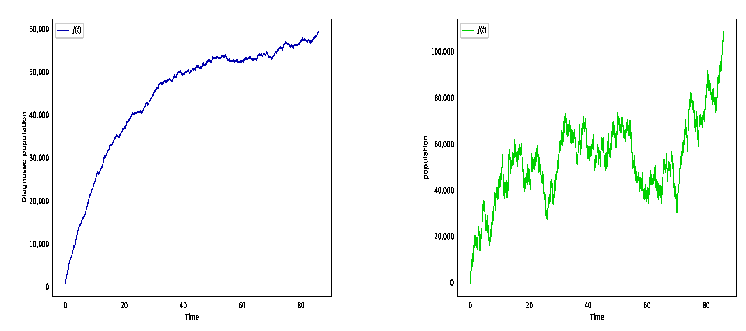
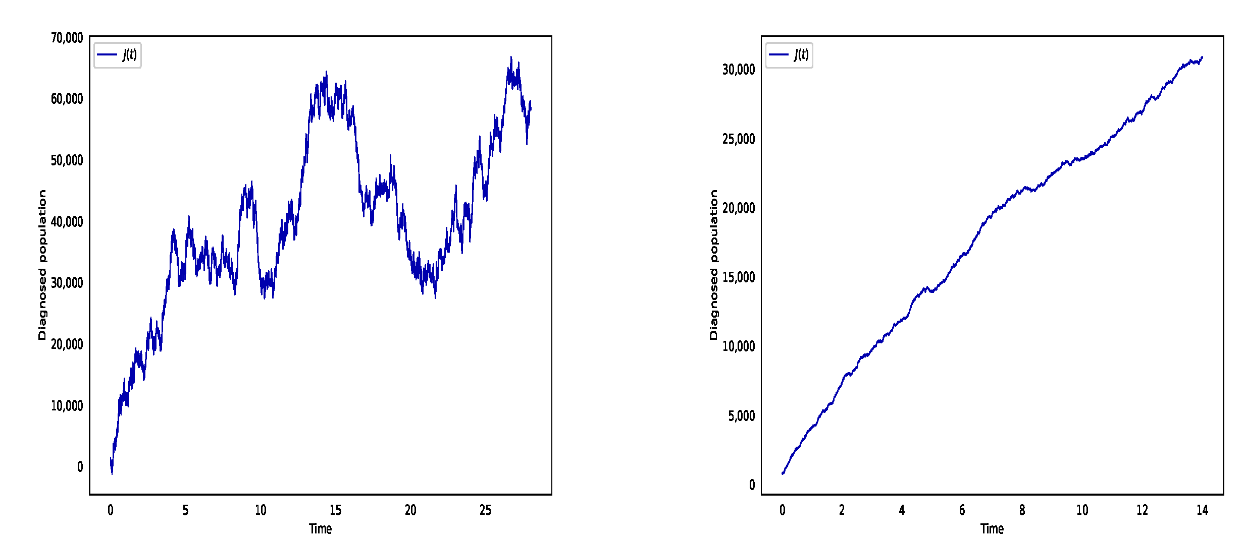
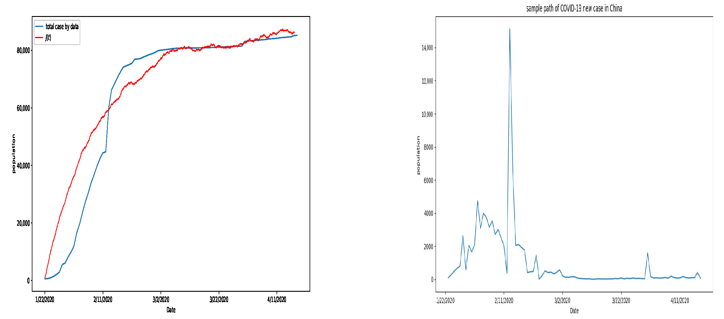
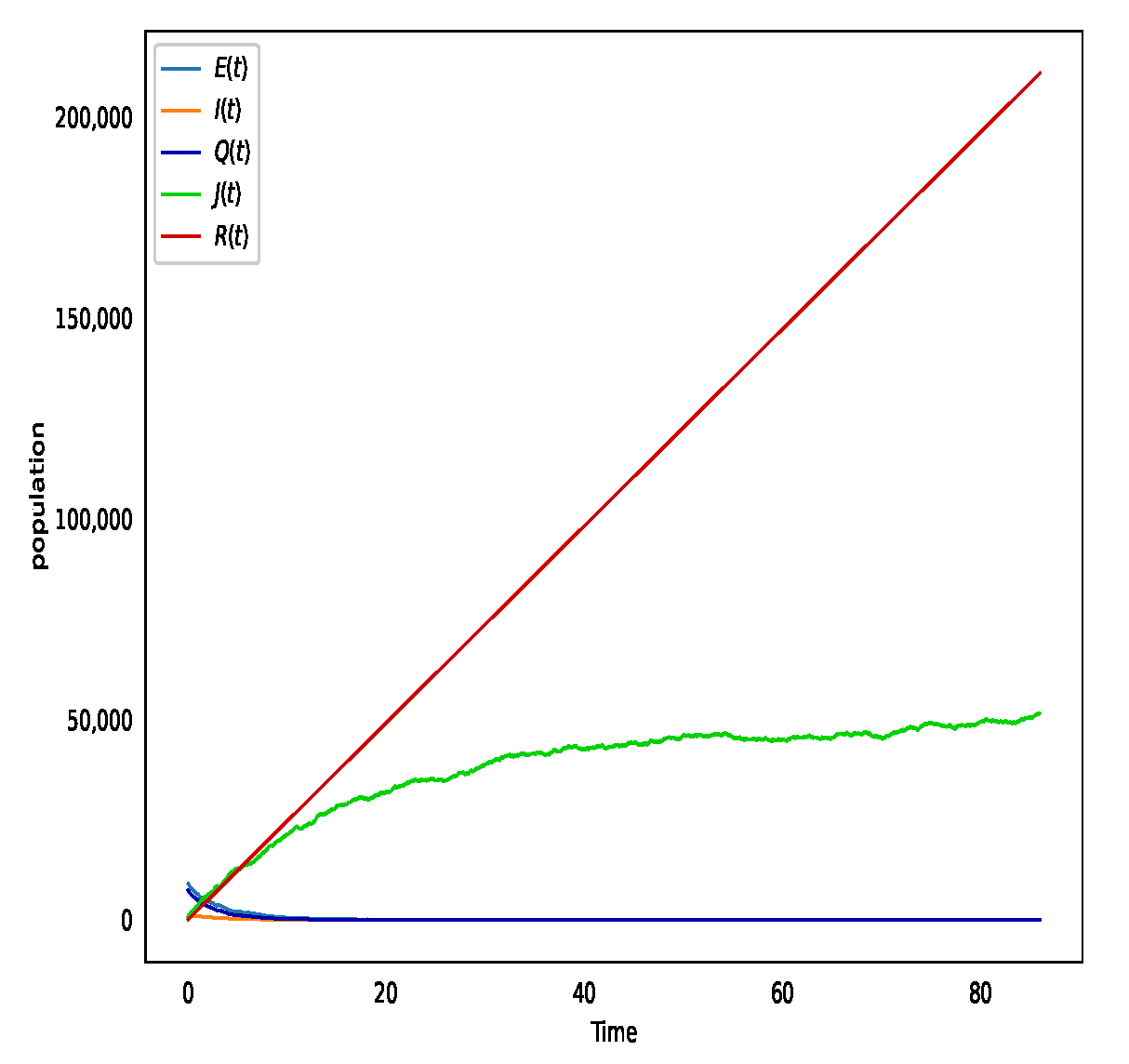
6. Numerical Simulation

Numerically, we will consider the numerical method given in [38] to approximate the proposed system (2) as follows:

$$\begin{array}{cc}\hfill E_{i+1}& =E_i+({\beta }_i(k{E}_i+I_i)-(\epsilon +\lambda )E_i)h-{\alpha }_1{E}_i\sqrt{h}{\xi }_i^j+\frac{1}{2}{\alpha }_1^2{E}_i(h{\left({\xi }_i^j\right)}^2-h),\hfill \\ \hfill I_{i+1}& =I_i+(\epsilon E_i-(\delta +\theta )I_i)h+{\alpha }_1{E}_i\sqrt{h}{\xi }_i^j,\hfill \\ \hfill Q_{i+1}& =Q_i+(\lambda E_i-\sigma Q_i)h-{\alpha }_2{Q}_i\sqrt{h}{\xi }_i^j+\frac{1}{2}{\alpha }_2^2{Q}_i(h{\left({\xi }_i^j\right)}^2-h),\hfill \\ \hfill J_{i+1}& =J_i+(\theta I_i+\sigma Q_i-(\delta +\gamma )J_i)h+{\alpha }_2{Q}_i\sqrt{h}{\xi }_i^j,\hfill \\ \hfill R_{i+1}& =R_i+\gamma J_{i}h,\hfill \end{array}$$

(26)

where ${\xi }_i^j,j=1,2$ are independent Gaussian random variables $N(0,1)$. Although the outbreak is not over, the spread of COVID-19 in China has been basically controlled in March. So, we have collected data between 23 January and 18 April 2020 in order to estimate the parameters in the model. The parameters of the stochastic EIQJR model are estimated following [39], then the numerical approximations are performed. We assume that the average latent period is 4 days [40], which means that the first symptom appears on the fifth day as a result of infection. Thus, we assume that the time from infection to diagnosis is 7 days, with the first 4 days in the exposed case having low infectivity and the last 3 days in the infected case having high infectivity. The proportion k is assumed to be 0.3. $94.3\%$ of the diagnosed COVID-19 cases come from the quarantined class, whereas the remaining $5.7\%$ come from the infected classes that have not been quarantined [40]. So,

$$\epsilon =\frac{1}{4}\frac{5.7}{100},\lambda =\frac{1}{4}\frac{94.3}{100},\theta =\frac{1}{3},\sigma =\frac{1}{3}.$$

Infected individuals will recover after 21 days on average, so we choose $\gamma =\frac{1}{21}$. The period of death for COVID-19 patients is 17 days, and the average death rate is $6.1\%$, and hence $\delta =\frac{1}{17}\frac{6.1}{100}$. Since the transmission rate $\beta \left(t\right)$ vary $t\in [0,86]$, we try to fix the function based on [41]. We assume that the transmission rate is $0.523$ before 20 February and $0.009$ after 20 February as a result of intervention strategies. From the data of [42], we estimate the initial values $E\left(0\right)=9000,I\left(0\right)=1240,Q\left(0\right)=7347,J\left(0\right)=771,R\left(0\right)=34$ as of 23 January 2020. We choose ${\alpha }_1,{\alpha }_2\in [0,1]$. We perform numerical simulations to certify our models, to discuss the transmission of COVID-19 and the effectiveness of control measures in China.

We carry out the simulation for different values of ${\alpha }_1$ and ${\alpha }_2$ to determine the impact of environmental noises while leaving the other parameters unchanged. In Figure 1, we choose ${\alpha }_1=0.09$, ${\alpha }_2=0.07$ (left) and ${\alpha }_1=0.95,{\alpha }_2=0.95$ (right). We see that the smaller noise has slight impact in the population whereas the larger white noises create more violent fluctuation curves and increase in infected population. Therefore the increases in environmental forcing may result in a reduction in the average time to extinction.

Figure 1. The numbers of diagnosed case with different noises. In particular, ${\alpha }_1=0.09,{\alpha }_2=0.07$ in (left) and ${\alpha }_1=0.95,{\alpha }_2=0.95$ in (right). It depicts that fluctuation is getting smaller with the decrease of the noise.

Figure 2 depicts the diagnosed populations at two time ranges: from 23 January to 20 February, and from 20 February to 6 March. At the transmission rate $5.23$ and $\delta =9.61,{\alpha }_1=0.95,{\alpha }_2=0.95$, Figure 2 (left) illustrates that the final diagnosed population is 68,000 as the result of few preventive and control measures before 20 February 2020. Due to the stringent control measure, the transmission rate and death rates decrease to $\delta =\frac{1}{17}\frac{0.67}{100},k=0.1,{\alpha }_1=0.09,{\alpha }_2=0.07$, and transmission rate is $0.009$ and result in the diagnosed case is 30,000 in the right side of Figure 2.

Figure 2. The numbers of diagnosed patient between 23 January and 20 February (left), and between 20 February and 6 March (right).

On the left side of Figure 3, the blue line is the statistical data reported (by Kaggle), the fluctuation curve is the prediction of the model. In the fluctuation curve, we choose ${\alpha }_1=0.05,{\alpha }_2=0.07,$ the transmission rate is $0.87$ and the other parameters are unchanged. The prediction curve relates to the actual data well. This figure illustrates the disease persists in the population. The right side of Figure 3 illustrates the daily new case in China, and it is suggested that the COVID-19 infection is stochastic.

Figure 3. Prediction and actual accumulated cases in China (left) and new confirmed cases in China (right).

In Figure 4, choose ${\alpha }_1=0.09,{\alpha }_2=0.07,k=0.1$ and transmission rate is $0.009$, then $\mu +\epsilon >{\beta }^{*}+{\alpha }_1^2,\sigma >\frac{3}{2}{\alpha }_2^2$. That is to say, the disease-free equilibrium condition is satisfied; therefore according to Theorem 2, Figure 4 depicts that $P^0$ is globally asymptotically stable.

Figure 4. The solution of system (2) when $\epsilon +\lambda >{\beta }^{*}k+{\alpha }_1^2$ and $\sigma >\frac{3}{2}{\alpha }_2^2$. It depicts the disease-free equilibrium $P^0$ is stable.

7. Discussion

In this paper, we propose and analyze a stochastic EIQJR model, which is an extension of deterministic model studied by Zhou and Ma [12]. We have investigated how stochastic perturbations in transmission coefficient $\epsilon$ and the diagnosis coefficient $\sigma$ affect the population dynamics of COVID-19. We have developed the analysis of the model in both theoretical and numerical ways.

First, we have shown that the proposed model has a global positive solution. Our Theorems 2 and 3 extend the corresponding Theorem 2 (if $R_0<1$, the disease die out) in [12]. For the stochastic dynamics of our model (2), we obtain the sufficient condition of the extinction of the disease, namely, if $R_0\le 1$, $\epsilon +\lambda -{\beta }^{*}k-{\alpha }_1^2>0$ and $\sigma >\frac{3}{2}{\alpha }_2^2$ hold, then the disease-free equilibrium is global asymptotic stability (see, Theorems 2 and 3). We have also examined the population behavior of system (2) around the endemic equilibrium of the deterministic system if $R_0>1$, $\epsilon +\lambda >{\alpha }_1^2$, and $\sigma >\frac{3}{2}{\alpha }_2^2$ hold. Comparing the previous deterministic model with our model (2), we find out that the presence of stochastic perturbation can restrain the spread of the disease. Epidemiologically, we can conclude that the volatility of the infected population rises with increasing noise intensity, and that environmental noises can maintain the irregular repetition of disease.

We have carried out numerical simulation to support theoretical results and to show the transmission process of COVID-19 in China. Numerical results suggest that disease-free equilibrium is global asymptotic stability under suitable conditions (see, Figure 4). In Figure 1 and Figure 2, our results suggest that the increase of ${\alpha }_1$ and ${\alpha }_2$ and transmission rate might cause the volatility of infected population. Figure 3 suggests that our prediction curve fits the actual data, and we can see that COVID-19 infection is stochastic. Because the explicit solutions are available in numerical analysis, it is interesting for one to consider a numerical method for stochastic EIQJR models. Some scholars have already worked in the literature (e.g., ([43,44,45])). We leave these investigations for future work.

References

- World Health Organization. Coronavirus. Available online: https://www.who.int/health-topics/coronavirus (accessed on 19 January 2020).
- World Health Organization. Naming the Coronavirus Disease (COVID-2019) and the Virus That Causes It. Available online: https://www.who.int/emergencies/diseases/novel-coronavirus-2019/technical-guidance/naming-the-coronavirus-disease-(covid-2019)-and-the-virus-that-causes-it#:~:text=Human (accessed on 24 February 2020).
- Gorbalenya, A.E.B. Severe acute respiratory syndrome-related coronavirus: The species and its viruses, a statement of the Coronavirus Study Group. bioRxiv 2020. [Google Scholar]
- Gao, Q.; Hu, Y.; Dai, Z.; Xiao, F.; Wang, J.; Wu, J. The epidemiological characteristics of 2019 novel coronavirus diseases (COVID-19) in Jingmen, Hubei, China. Medicine 2020, 99, e20605. [Google Scholar] [CrossRef] [PubMed]
- Thinley, P. Technical comments on the design and designation of biological corridors in Bhutan: Global to national perspectives. J. Renew. Nat. Resour. Bhutan 2010, 6, 91–106. [Google Scholar]
- World Health Organization. Coronavirus Disease 2019. 2020. Available online: https://www.who.int/emergencies/diseases/novel-coronavirus-2019 (accessed on 18 June 2020).
- How Does Coronavirus Spread? NBC News, 29 January 2020.
- U.S. Centers for Disease Control and Prevention (CDC). How COVID-19 Spreads. Available online: https://www.cdc.gov/coronavirus/2019-ncov/about/transmission.html (accessed on 27 January 2020).
- World Health Organization. Getting Your Workplace Ready for COVID-19. Available online: https://www.who.int/docs/default-source/searo/thailand/getting-your-workplace-ready-for-covid19.pdf?sfvrsn=1a068386_0 (accessed on 3 March 2020).
- Wang, F.S.; Zhang, C. What to do next to control the 2019-nCoV epidemic? Lancet 2020, 395, 391–393. [Google Scholar] [CrossRef]
- Li, Q.; Guan, X.; Wu, P.; Wang, X.; Zhou, L.; Tong, Y.; Feng, Z. Early transmission dynamics in Wuhan, China, of novel coronavirus-infected pneumonia. N. Engl. J. Med. 2020, 382, 1199–1207. [Google Scholar] [CrossRef]
- Zhou, Y.; Ma, Z. A discrete epidemic model for SARS transmission and control in china. Math. Comput. Model. 2004, 40, 1491–1506. [Google Scholar] [CrossRef]
- Lin, Q.; Zhao, S.; Gao, D.; Lou, Y.; Yang, S.; Musa, S.S.; Wang, M.H.; Cai, Y.; Wang, W.; Yang, L.; et al. A conceptual model for the coronavirus disease 2019 (COVID-19) outbreak in Wuhan, China with individual reaction and government action. Int. J. Infect. Dis. 2020, 93, 211–216. [Google Scholar] [CrossRef]
- Chen, T.M.; Rui, J.; Wang, Q.P.; Zhao, Z.Y.; Cui, J.A.; Yin, L. A mathematical model for simulating the phase-based transmissibility of a novel coronavirus. Infect. Dis. Poverty 2020, 9, 1–8. [Google Scholar] [CrossRef]
- Tang, S.; Xiao, Y.; Yuan, L.; Cheke, R.A.; Wu, J. Campus quarantine (Fengxiao) for curbing emergent infectious diseases: Lessons from mitigating A/H1N1 in Xian, China. J. Theor. Biol. 2012, 295, 47–58. [Google Scholar] [CrossRef]
- Xiao, Y.; Tang, S.; Wu, J. Media impact switching surface during an infectious disease outbreak. Sci. Rep. 2015, 5, 1–9. [Google Scholar] [CrossRef]
- Wu, J.T.; Leung, K.; Leung, G.M. Nowcasting and forecasting the potential domestic and international spread of the 2019-nCoV outbreak originating in Wuhan, China: A modelling study. Nat. Med. 2020, 395, 689–697. [Google Scholar] [CrossRef]
- Zeb, A.; Alzahrani, E.; Erturk, V.S.; Zaman, G. Mathematical model for coronavirus disease 2019 (COVID-19) containing isolation class. BioMed Res. Int. 2020, 2020, 3452402. [Google Scholar] [CrossRef] [PubMed]
- Allen, L.J. Some discrete-time SI, SIR, and SIS epidemic models. Math. Biosci. 1994, 124, 83–105. [Google Scholar] [CrossRef]
- Jamshidi, S.; Baniasad, M.; Niyogi, D. Global to USA county scale analysis of weather, urban density, mobility, homestay, and mask use on COVID-19. Int. J. Environ. Res. Public Health 2020, 17, 7847. [Google Scholar] [CrossRef]
- Keeling, M.; Rohani, P. Modeling Infectious Diseases in Human and Animals; Princeton University Press: Princeton, NJ, USA, 2008. [Google Scholar] [CrossRef]
- Ikram, R.; Khan, A.; Zahri, M.; Saeed, A.; Yavuz, M.; Kumam, P. Extinction and stationary distribution of a stochastic COVID-19 epidemic model with time-delay. Comput. Biol. Med. 2022, 141, 105115. [Google Scholar] [CrossRef]
- Mao, X.; Marion, G.; Renshaw, E. Environmental brownian noise suppresses explosions in population dynamics. Stoch. Process. Their Appl. 2002, 97, 95–110. [Google Scholar] [CrossRef]
- Britton, T. Stochastic epidemic models: A survey. Math. Biosci. 2010, 225, 24–35. [Google Scholar] [CrossRef]
- Ji, C.; Jiang, D.; Shi, N. The behavior of an SIR epidemic model with stochastic perturbation. Stoch. Anal. Appl. 2012, 30, 755–773. [Google Scholar] [CrossRef]
- Tornatore, E.; Buccellato, S.M.; Vetro, P. Stability of a stochastic SIR system. Phys. A 2005, 354, 111–126. [Google Scholar] [CrossRef]
- Tornatore, E.; Vetro, P.; Buccellato, S.M. SIVR epidemic model with stochastic perturbation. Neural Comput. Appl. 2014, 24, 309–315. [Google Scholar] [CrossRef]
- Lahrouz, A.; Omari, L.; Kiouach, D. Global analysis of a deterministic and stochastic nonlinear SIRS epidemic model. Nonlinear Anal. Model. Control 2011, 16, 59–76. [Google Scholar] [CrossRef] [Green Version]
- Hou, T.; Lan, G.; Yuan, S.; Zhang, T. Threshold dynamics of a stochastic SIHR epidemic model of COVID-19 with general population-size dependent contact rate. Math. Biosci. Eng. 2022, 19, 4217–4236. [Google Scholar] [CrossRef] [PubMed]
- Hussain, S.; Madi, E.N.; Khan, H.; Etemad, S.; Rezapour, S.; Sitthiwirattham, T.; Patanarapeelert, N. Investigation of the stochastic modeling of COVID-19 with environmental noise from the analytical and numerical point of view. Mathematics 2021, 9, 3122. [Google Scholar] [CrossRef]
- Tesfaye, A.W.; Satana, T.S. Stochastic model of the transmission dynamics of COVID-19 pandemic. Adv. Differ. Equ. 2021, 2021, 457. [Google Scholar] [CrossRef] [PubMed]
- Zhang, Z.; Zeb, A.; Hussain, S.; Alzahrani, E. Dynamics of COVID-19 mathematical model with stochastic perturbation. Adv. Differ. Equ. 2020, 2020, 451. [Google Scholar] [CrossRef] [PubMed]
- Ding, Y.; Fu, Y.; Kang, Y. Stochastic analysis of COVID-19 by a SEIR model with lévy noise. Chaos Interdiscip. J. Nonlonear Sci. 2021, 31, 043132. [Google Scholar] [CrossRef]
- Nino-Torres, D.; Rios-Gutierrez, A.; Arunachalam, V.; Ohajunwa, C.; Seshaiyer, P. Stochastic modelling, analysis, and simulation of the COVID-19 pandemic with explicit behavioral changes in Bogota: A case study. Infect. Dis. Model. 2022, 7, 199–211. [Google Scholar] [CrossRef]
- Tesfay, A.; Saeed, T.; Zeb, A.; Tesfay, D.; Khalaf, A.; Brannan, J. Dynamics of a stochastic COVID-19 epidemic model with jump-diffusion. Adv. Differ. Equ. 2021, 2021, 228. [Google Scholar] [CrossRef]
- Arnold, L. Stochastic Differential Equations: Theory and Applications; Wiley: Hoboken, NJ, USA, 1972. [Google Scholar]
- Mao, X. Stochastic Differential Equations and Applications; Horwood: Chichester, UK, 1997. [Google Scholar]
- Kingi, H. Numerical SDE Simulation-Euler vs. Milstein Methods. Available online: https://hautahi.com/sde-simulation (accessed on 31 December 2019).
- Zhang, W.; Du, R.; Li, B.; Zheng, X.; Yang, X.; Hu, B.; Wang, Y.; Xiao, G.; Yan, B.; Shi, Z.; et al. Molecular and serological investigation of 2019-nCoV infected patients: Implication of multiple shedding routes. Emerg. Microbes Infect. 2020, 9, 386–389. [Google Scholar] [CrossRef]
- Mi, Y.; Huang, T.; Zhang, J.; Qin, Q.; Gong, Y.; Liu, S.; Xue, H.; Ning, C.; Cao, L.; Cao, Y. Estimating instant case fatality rate of COVID-19 in China. Int. J. Infect. Dis. 2020, 97, 1–6. [Google Scholar] [CrossRef]
- Zhang, X.-S.; Vynnycky, E.; Charlett, A.; Angelis, D.D.; Chen, Z.; Liu, W. Transmission dynamics and control measures of COVID-19 outbreak in China: A modelling study. Sci. Rep. 2021, 11, 2652. [Google Scholar] [CrossRef] [PubMed]
- Tang, B.; Xia, F.; Tang, S.; Bragazzi, N.L.; Li, Q.; Sun, X.; Liang, J.; Xiao, Y.; Wu, J. The effectiveness of quarantine and isolation determine the trend of the COVID-19 epidemic in the final phase of the current outbreak in China. Int. J. Infect. Dis. 2020, 96, 636–647. [Google Scholar] [CrossRef] [PubMed]
- Eissa, M.A.; Zhang, H.; Xiao, Y. Mean-square stability of split-step theta milstein methods for stochastic differential equaitons. Math. Probl. Eng. 2018, 2018, 1682513. [Google Scholar] [CrossRef]
- Eissa, M.A. Mean-square stability of two classes of theta milstein methods for nonlinear stochastic differential equations. Proc. Jangjeon Math. Soc. 2019, 22, 119–128. [Google Scholar]
- Eissa, M.A.; Ye, Q. Convergence, nonnegativity and stability of a new Lobatto IIIC-Milstein method for a pricing option approach based on stochastic volatility model. Jpn. J. Ind. Appl. Math. 2021, 38, 391–424. [Google Scholar] [CrossRef]
Publisher’s Note: MDPI stays neutral with regard to jurisdictional claims in published maps and institutional affiliations. |
© 2022 by the authors. Licensee MDPI, Basel, Switzerland. This article is an open access article distributed under the terms and conditions of the Creative Commons Attribution (CC BY) license (https://creativecommons.org/licenses/by/4.0/).