
Stationary Probability Density Analysis for the Randomly Forced Phytoplankton–Zooplankton Model with Correlated Colored Noises

Abstract
:1. Introduction
2. Model Formulation
- (i)
- In the absence of zooplankton, the growth of TPP population follows the logistic law with intrinsic growth rate r and environmental carrying capacity K.
- (ii)
- In the absence of limiting factors, the chance of an individual zooplankton encountering prey is proportional to its abundance, so the predation rate is assumed to obey the simple law of mass action. On the other hand, no matter how large the TPP population is, each zooplankton individual has a maximum consumption rate. Therefore, in the presence of toxic algae, the more common choice is the Holling type II functional response to describe this grazing phenomena [13].
- (iii)
- TPP population is directly affected by anthropogenic toxins, while zooplankton population feeding on contaminated TPP is indirectly affected by toxins [21].
- (iv)
3. Stochastic Analysis of The Model
4. Numerical Simulation
5. Discussion
- •
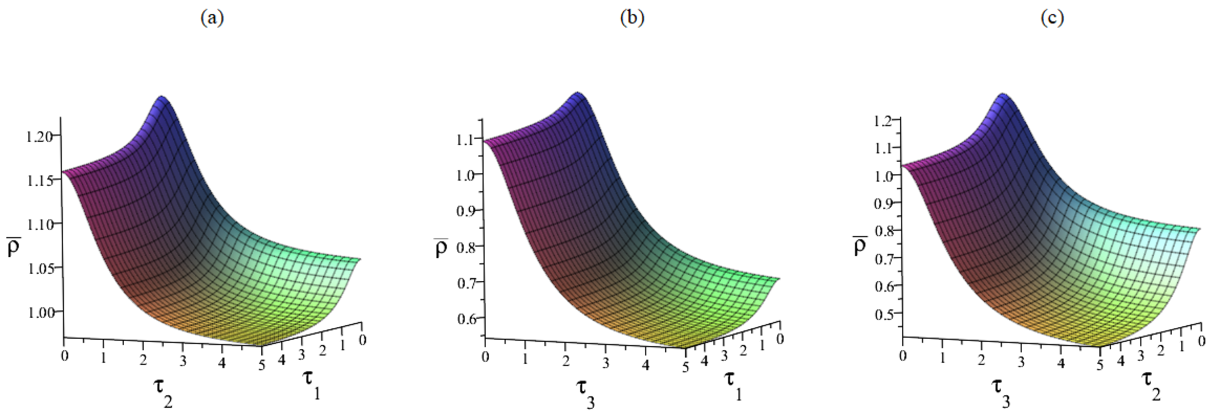
- The noise intensity , the correlation time () and the coefficient of anthropogenic toxicity may reduce the level of , namely, the distribution range of population density will be more concentrated with the increase in , (), and . Ecologically, these parameters are favorable for maintaining a balanced plankton population, which may seem counterintuitive.
- •
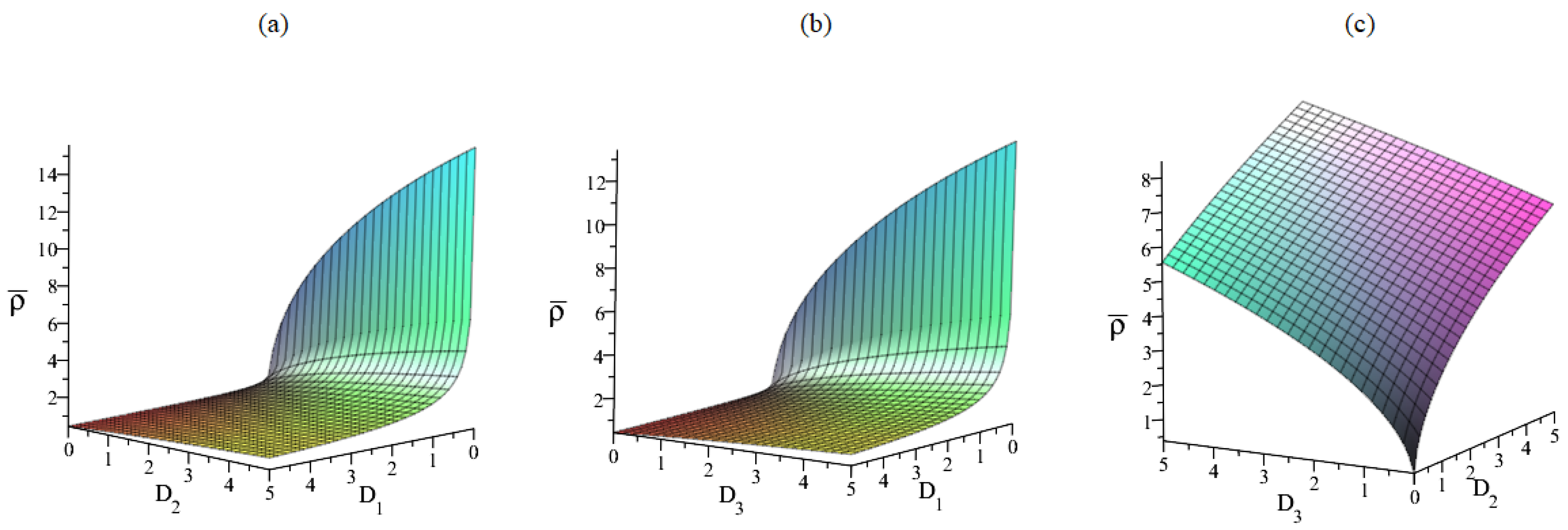
- The noise intensities and can enhance the level of , which implies that the distribution range of population density will be enlarged with the increase in and . As a result, they weaken the stability of the system.
- •
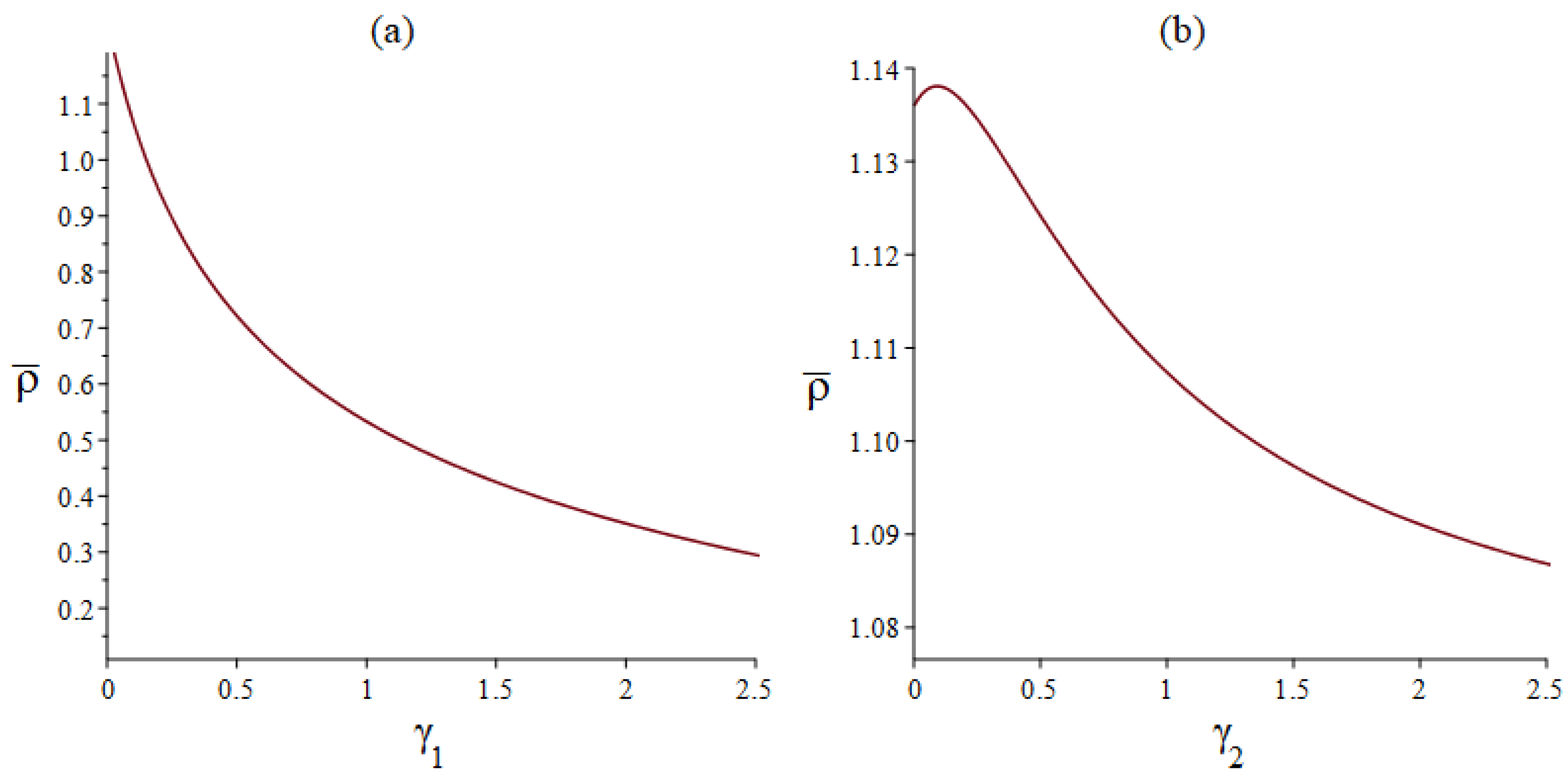
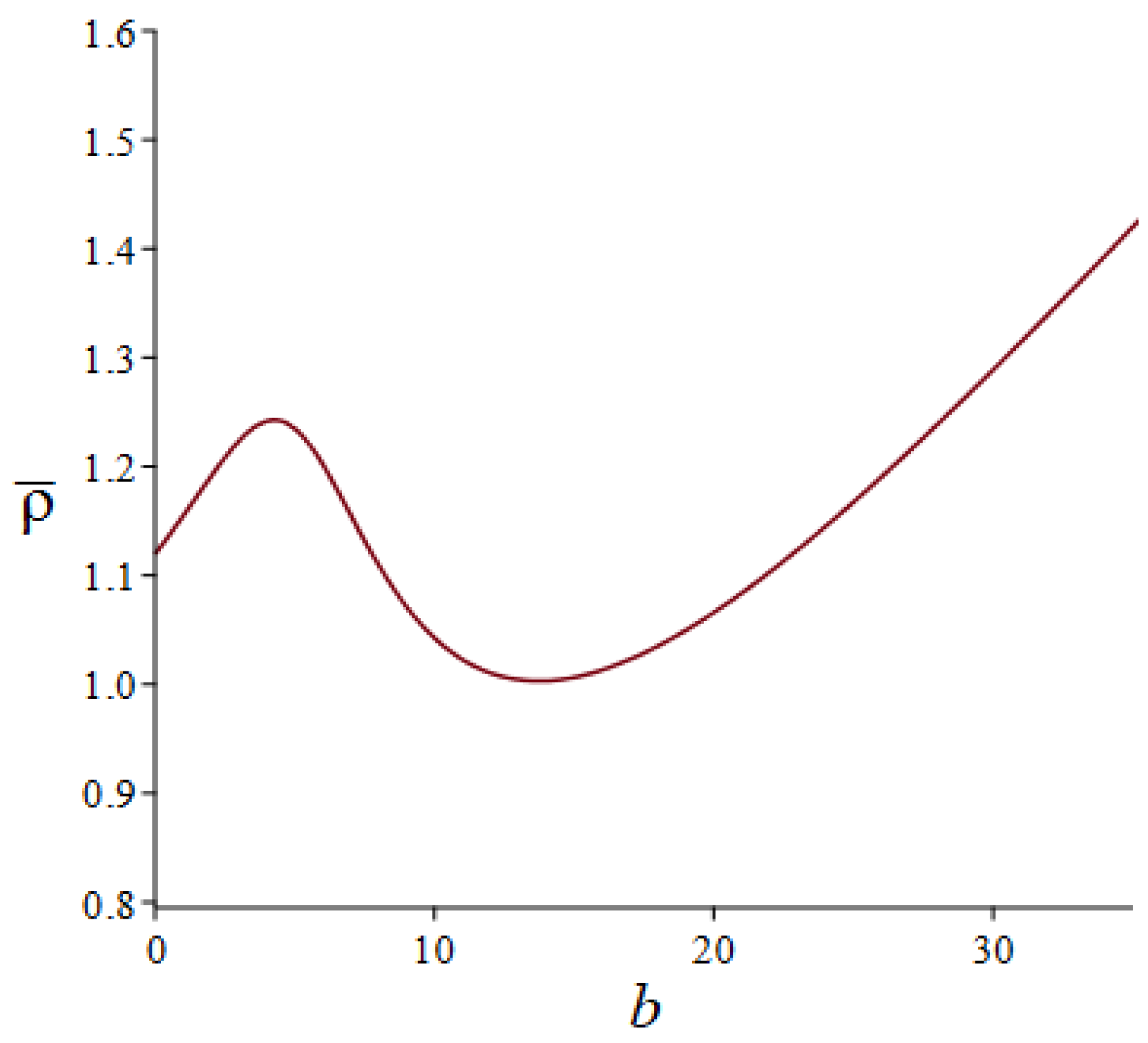
- The influence of anthropogenic toxicity coefficient and the toxin release rate by TPP population b is more complicated, depending on the content of the two toxins. In other words, these two parameters can be used as a means of controlling algal blooms.
Author Contributions
Funding
Institutional Review Board Statement
Informed Consent Statement
Data Availability Statement
Conflicts of Interest
References
- Bharathi, M.; Venkataramana, V.; Sarma, V. Phytoplankton community structure is governed by salinity gradient and nutrient composition in the tropical estuarine system. Cont. Shelf. Res. 2022, 234, 104643. [Google Scholar] [CrossRef]
- Sekerci, Y.; Petrovskii, S. Mathematical modelling of plankton-oxygen dynamics under the climate change. Bull. Math. Biol. 2015, 77, 2325–2353. [Google Scholar] [CrossRef] [PubMed] [Green Version]
- Agnihotri, K.; Kaur, H. The dynamics of viral infection in toxin producing phytoplankton and zooplankton system with time delay. Chaos Solitons Fractals 2019, 118, 122–133. [Google Scholar] [CrossRef]
- Niu, Y.; Liu, C.; Lu, X.; Zhu, L.; Sun, Q.; Wang, S. Phytoplankton blooms and its influencing environmental factors in the southern Yellow Sea. Reg. Stud Mar. Sci. 2021, 47, 101916. [Google Scholar] [CrossRef]
- Bao, L.; Chen, J.; Tong, H.; Qian, J.; Li, X. Phytoplankton dynamics and implications for eutrophication management in an urban river with a series of rubber dams. J. Environ. Manag. 2022, 311, 114865. [Google Scholar] [CrossRef]
- Ghanbari, B.; Gómez-Aguilar, J. Modeling the dynamics of nutrient-phytoplankton-zooplankton system with variable-order fractional derivatives. Chaos Soliton. Fract. 2018, 116, 114–120. [Google Scholar] [CrossRef]
- Schweigert, J.; Thompson, M.; Fort, C.; Hay, D.E.; Therriault, T.W.; Brown, L.N. Factors linking Pacific herring (Clupea pallasi) productivity and the spring plankton bloom in the Strait of Georgia, British Columbia, Canada. Prog. Oceanogr. 2013, 115, 103–110. [Google Scholar] [CrossRef]
- Niu, L.; Van Gelder, P.; Zhang, C.; Guan, Y.; Vrijling, J.K. Physical control of phytoplankton bloom development in the coastal waters of Jiangsu (China). Ecol. Model. 2016, 321, 75–83. [Google Scholar] [CrossRef]
- Sohma, A.; Imada, R.; Nishikawa, T.; Shibuki, H. Modeling the life cycle of four types of phytoplankton and their bloom mechanisms in a benthic-pelagic coupled ecosystem. Ecol. Model. 2022, 467, 109882. [Google Scholar] [CrossRef]
- Kumar, B.; Bhaskararao, D.; Krishna, P. Impact of nutrient concentration and compositionon shifting of phytoplankton community in the coastal waters of the Bay of Bengal. Reg. Stud. Mar. Sci. 2022, 51, 102228. [Google Scholar] [CrossRef]
- Zhao, Q.; Liu, S.; Niu, X. Effect of water temperature on the dynamic behavior of phytoplankton-zooplankton model. Appl. Math. Comput. 2020, 378, 125211. [Google Scholar] [CrossRef]
- Chen, M.; Fan, M.; Liu, R.; Wang, X.; Yuan, X.; Zhu, H. The dynamics of temperature and light on the growth of phytoplankton. J. Theor. Biol. 2015, 385, 8–19. [Google Scholar] [CrossRef] [PubMed]
- Chattopadhayay, J.; Sarkar, R.R.; Mandal, S. Toxin-producing plankton may act as a biological control for planktonic blooms-field study and mathematical modelling. J. Theor. Biol. 2002, 215, 333–344. [Google Scholar] [CrossRef] [PubMed] [Green Version]
- Pal, R.; Basu, D.; Banerjee, M. Modelling of phytoplankton allelopathy with Monod-Haldane-type functional response-a mathematical study. Biosystems 2009, 95, 243–253. [Google Scholar] [CrossRef] [PubMed]
- Scotti, T.; Mimura, M.; Wakano, J.Y. Avoiding toxic prey may promote harmful algal blooms. Ecol. Complex. 2015, 21, 157–165. [Google Scholar] [CrossRef]
- Jang, S.; Baglama, J.; Wu, L. Dynamics of phytoplankton-zooplankton systems with toxin producing phytoplankton. Appl. Math. Comput. 2014, 227, 717–740. [Google Scholar] [CrossRef]
- Han, R.; Dai, B. Spatiotemporal pattern formation and selection induced by nonlinear cross-diffusion in a toxic-phytoplankton-zooplankton model with Allee effect. Nonlinear Anal. Real World Appl. 2019, 45, 822–853. [Google Scholar] [CrossRef]
- Peng, Y.; Li, Y.; Zhang, T. Global bifurcation in a toxin producing phytoplankton-zooplankton system with prey-taxis. Nonlinear Anal. Real World Appl. 2021, 61, 103326. [Google Scholar] [CrossRef]
- Liu, C.; Yu, L.; Zhang, Q.; Li, Y. Dynamic analysis of a hybrid bioeconomic plankton system with double time delays and stochastic fluctuations. Appl. Math. Comput. 2018, 316, 115–137. [Google Scholar] [CrossRef]
- Walker, C.H.; Sibly, R.M.; Hopkin, S.H.; Peakall, D.B. Principles of Ecotoxicology; CRC Press: Boca Raton, FL, USA, 2012. [Google Scholar]
- Das, T.; Mukherjee, R.N.; Chaudhuri, K.S. Harvesting of a prey-predator fishery in the presence of toxicity. Appl. Math. Model. 2009, 33, 2282–2292. [Google Scholar] [CrossRef]
- Chakraborty, K.; Das, K. Modeling and analysis of a two-zooplankton one-phytoplankton system in the presence of toxicity. Appl. Math. Model. 2015, 39, 1241–1265. [Google Scholar] [CrossRef]
- Huang, Q.; Wang, H.; Lewis, M.A. The impact of environmental toxins on predator-prey dynamics. J. Theor. Biol. 2015, 378, 12–30. [Google Scholar] [CrossRef]
- May, R. Stability and Complexity in Model Ecosystems; Princeton University Press: Princeton, NJ, USA, 1973. [Google Scholar]
- Qi, H.; Meng, X.; Hayat, T.; Hobiny, A. Stationary distribution of a stochastic predator-prey model with hunting cooperation. Appl. Math. Lett. 2022, 1124, 107662. [Google Scholar] [CrossRef]
- Li, D.; Liu, S.; Cui, J. Threshold dynamics and ergodicity of an SIRS epidemic model with semi-Markov switching. J. Differ. Equ. 2019, 266, 3973–4017. [Google Scholar] [CrossRef]
- Liu, M. Optimal harvesting of stochastic population models with periodic coefficients. J. Nonlinear Sci. 2022, 32, 23. [Google Scholar] [CrossRef]
- Song, M.; Zuo, W.; Jiang, D.; Hayat, T. Stationary distribution and ergodicity of a stochastic cholera model with multiple pathways of transmission. J. Frankl. Inst. 2020, 357, 10773–10798. [Google Scholar] [CrossRef]
- Li, X.; Liu, W.; Mao, X.; Zhao, J. Stabilization and destabilization of hybrid systems by periodic stochastic controls. Syst. Control Lett. 2021, 152, 104929. [Google Scholar] [CrossRef]
- He, S.; Tang, S.; Cai, Y.; Wang, W.; Rong, L. A stochastic epidemic model coupled with seasonal air pollution: Analysis and data fitting. Stoch. Environ. Res. Risk Assess. 2020, 34, 2245–2257. [Google Scholar] [CrossRef]
- Nguyen, D.; Yin, G.; Zhu, C. Long-term analysis of a stochastic SIRS model with general incidence rates. SIAM J. Appl. Math. 2020, 80, 814–838. [Google Scholar] [CrossRef] [Green Version]
- Yu, X.; Ma, Y. An avian influenza model with nonlinear incidence and recovery rates in deterministic and stochastic environments. Nonlinear Dyn. 2022, 108, 4611–4628. [Google Scholar] [CrossRef]
- Sarkar, R.R.; Chattopadhayay, J. The role of environmental stochasticity in a toxic phytoplankton-non-toxic phytoplankton-zooplankton system. Environmetrics 2003, 14, 775–792. [Google Scholar] [CrossRef]
- Chen, Z.; Zhang, R.; Li, J.; Zhang, S.; Wei, C. A stochastic nutrient-phytoplankton model with viral infection and Markov switching. Chaos Solitons Fractals 2020, 140, 110109. [Google Scholar] [CrossRef]
- Jang, S.; Allen, E. Deterministic and stochastic nutrient-phytoplankton-zooplankton models with periodic toxin producing phytoplankton. Appl. Math. Comput. 2015, 271, 52–67. [Google Scholar] [CrossRef]
- Song, D.; Fan, M.; Yan, S.; Liu, M. Dynamics of a nutrient-phytoplankton model with random phytoplankton mortality. J. Theor. Biol. 2020, 488, 110119. [Google Scholar] [CrossRef] [PubMed]
- Wang, H.; Jiang, D.; Hayat, T.; Alsaedi, A.; Ahmad, B. Stationary distribution of stochastic NP ecological model under regime switching. Phys. A 2020, 549, 124064. [Google Scholar] [CrossRef]
- Sarkar, R.R.; Chattopadhayay, J. Occurrence of planktonic blooms under environmental fluctuations and its possible control mechanism-mathematical models and experimental observations. J. Theor. Biol. 2003, 224, 501–516. [Google Scholar] [CrossRef]
- Xu, C. Phenomenological bifurcation in a stochastic logistic model with correlated colored noises. Appl. Math. Lett. 2020, 101, 106064. [Google Scholar] [CrossRef]
- Hu, J.; Liu, Z. Incorporating two coupling noises into a nonlinear competitive system with saturation effect. Int. J. Biomath. 2020, 13, 2050012. [Google Scholar] [CrossRef]
- Tian, B.; Yang, L.; Chen, X.; Zhang, Y. A generalized stochastic competitive system with Ornstein-Uhlenbeck process. Int. J. Biomath. 2021, 14, 2150001. [Google Scholar] [CrossRef]
- Liao, T. The impact of plankton body size on phytoplankton-zooplankton dynamics in the absence and presence of stochastic environmental fluctuation. Chaos Solitons Fractals 2022, 154, 111617. [Google Scholar] [CrossRef]
- Yu, X.; Yuan, S.; Zhang, T. The effects of toxin-producing phytoplankton and environmental fluctuations on the planktonic blooms. Nonlinear Dyn. 2018, 91, 1653–1668. [Google Scholar] [CrossRef]
- Zhang, Y.; Zheng, Y.; Zhao, F.; Liu, X. Dynamical analysis in a stochastic bioeconomic model with stage-structuring. Nonlinear Dyn. 2016, 84, 1113–1121. [Google Scholar] [CrossRef]
- Denaro, G.; Valenti, D.; Spagnolo, B.; Basilone, G.; Mazzola, S.; Zgozi, S.W.; Aronica, S.; Bonanno, A. Dynamics of two picophytoplankton groups in mediterranean sea: Analysis of the deep chlorophyll maximum by a stochastic advection-reaction-diffusion model. PLoS ONE 2013, 8, e66765. [Google Scholar] [CrossRef] [PubMed]
- Caruso, A.; Gargano, M.E.; Valenti, D.; Fiasconaro, A.; Spagnolo, B. Cyclic fluctuations, climatic changes and role of noise in planktonic foraminifera in the mediterranean sea. Fluct. Noise Lett. 2005, 5, L349–L355. [Google Scholar] [CrossRef] [Green Version]
- Spagnolo, B.; Cirone, M.; Barbera, A.; de Pasquale, F. Noise-induced effects in population dynamics. J. Phys-Condens. Mat. 2002, 14, 2247–2255. [Google Scholar] [CrossRef]
- Huang, D.; Wang, H.; Feng, J.; Zhu, Z.W. Hopf bifurcation of the stochastic model on HAB nonlinear stochastic dynamics. Chaos Soliton. Fract. 2006, 27, 1072–1079. [Google Scholar] [CrossRef]
- Zeng, C.; Wang, H. Colored noise enhanced stability in a tumor cell growth system under immune response. J. Stat. Phys. 2010, 141, 889–908. [Google Scholar] [CrossRef]
- Guarcello, C.; Valenti, D.; Carollo, A.; Spagnolo, B. Stabilization effects of dichotomous noise on the lifetime of the superconducting state in a long Josephson junction. Entropy 2015, 17, 2862–2875. [Google Scholar] [CrossRef] [Green Version]
- Mikhaylov, A.; Pimashkin, A.; Pigareva, Y.; Gerasimova, S.; Gryaznov, E.; Shchanikov, S.; Zuev, A.; Talanov, M.; Lavrov, I.; Demin, V.; et al. Neurohybrid memristive CMOS-integrated systems for biosensors and neuroprosthetics. Front. Neurosci. 2020, 14, 358. [Google Scholar] [CrossRef]
- Wang, K.; Ju, L.; Wang, Y.; Li, S.H. Impact of colored cross-correlated non-Gaussian and Gaussian noises on stochastic resonance and stochastic stability for a metapopulation system driven by a multiplicative signal. Chaos Solitons Fractals 2018, 108, 166–181. [Google Scholar] [CrossRef]
- Fulinski, A.; Telejko, T. On the effect of interference of additive and multiplicative noises. Phys. Lett. A 1991, 152, 11–14. [Google Scholar] [CrossRef]
- Mei, D.; Xie, C.; Zhang, L. The stationary properties and the state transition of the tumor cell growth model. Eur. Phys. J. B 2004, 41, 107–112. [Google Scholar] [CrossRef]
- Madureira, A.J.R.; Haenggi, P.; Wio, H.S. Giant suppression of the activation rate in the presence of correlated white noise sources. Phys. Lett. A 1996, 217, 248–252. [Google Scholar] [CrossRef]
- Mantegna, R.N.; Spagnolo, B. Probability distribution of the residence times in periodically fluctuating metastable systems. Int. J. Bifurcat. Chaos 1998, 8, 783–790. [Google Scholar] [CrossRef]
- Mikhaylov, A.N.; Guseinov, D.V.; Belov, A.I.; Korolev, D.S.; Shishmakova, V.A.; Koryazhkina, M.N.; Filatov, D.O.; Gorshkov, O.N.; Maldonado, D.; Alonso, F.J.; et al. Stochastic resonance in a metal-oxide memristive device. Chaos Solitons Fractals 2021, 144, 110723. [Google Scholar] [CrossRef]
- Li, Y.G.; Xu, Y.; Kurths, J.; Yue, X. Lévy-noise-induced transport in a rough triple-well potential. Phys. Rev. E 2016, 94, 042222. [Google Scholar] [CrossRef]
- Guarcello, C.; Valenti, D.; Spagnolo, B.; Pierro, V.; Filatrella, G. Anomalous transport effects on switching currents of graphene-based Josephson junctions. Nanotechnology 2017, 28, 134001. [Google Scholar] [CrossRef] [PubMed] [Green Version]
- Carollo, A.; Valenti, D.; Spagnolo, B. Geometry of quantum phase transitions. Phys. Rep. 2020, 838, 1–72. [Google Scholar] [CrossRef] [Green Version]
- Ma, Y.; Yu, X. Stochastic stability and stationary probability density analysis for a nutrient-phytoplankton model with multiplicative and additive noises. Appl. Math. Lett. 2022, 132, 108201. [Google Scholar] [CrossRef]
- Yu, X.; Ma, Y. Steady-state analysis of the stochastic Beverton-Holt growth model driven by correlated colored noises. Chaos Soliton. Fract. 2022, 158, 112102. [Google Scholar] [CrossRef]
- Khasminskii, R. On the principle of averaging for Itô stochastic differential equations. Kybernetika (Prague) 1968, 4, 260–279. [Google Scholar]
- Zhu, W. Nonlinear Stochastic Dynamics and Control Hamilton Theory System Framework; Science Press: Beijing, China, 2003. [Google Scholar]
- Xu, Y.; Guo, R.; Jia, W.; Li, J. Stochastic averaging for a class of single degree of freedom systems with combined Gaussian noises. Acta Mech. 2014, 225, 2611–2620. [Google Scholar] [CrossRef]
- Namachchivaya, N. Stochastic bifurcation. Appl. Math. Comput. 1990, 38, 101–159. [Google Scholar]


| Parameter | Description |
|---|---|
| r | Intrinsic growth rate of TPP population |
| K | Environmental carrying capacity of TPP population |
| Rate of predation of zooplankton on TPP population | |
| Ratio of biomass consumed by zooplankton for its growth | |
| Mortality rate of zooplankton | |
| a | Half saturation constant |
| b | Rate of toxin liberation by TPP population |
| Coefficient of toxicity to phytoplankton | |
| Coefficient of toxicity to zooplankton |
Publisher’s Note: MDPI stays neutral with regard to jurisdictional claims in published maps and institutional affiliations. |
© 2022 by the authors. Licensee MDPI, Basel, Switzerland. This article is an open access article distributed under the terms and conditions of the Creative Commons Attribution (CC BY) license (https://creativecommons.org/licenses/by/4.0/).
Share and Cite
Ma, Y.; Yu, X. Stationary Probability Density Analysis for the Randomly Forced Phytoplankton–Zooplankton Model with Correlated Colored Noises. Mathematics 2022, 10, 2383. https://doi.org/10.3390/math10142383
Ma Y, Yu X. Stationary Probability Density Analysis for the Randomly Forced Phytoplankton–Zooplankton Model with Correlated Colored Noises. Mathematics. 2022; 10(14):2383. https://doi.org/10.3390/math10142383
Chicago/Turabian StyleMa, Yuanlin, and Xingwang Yu. 2022. "Stationary Probability Density Analysis for the Randomly Forced Phytoplankton–Zooplankton Model with Correlated Colored Noises" Mathematics 10, no. 14: 2383. https://doi.org/10.3390/math10142383
APA StyleMa, Y., & Yu, X. (2022). Stationary Probability Density Analysis for the Randomly Forced Phytoplankton–Zooplankton Model with Correlated Colored Noises. Mathematics, 10(14), 2383. https://doi.org/10.3390/math10142383