Electric-Vehicle Routing Planning Based on the Law of Electric Energy Consumption

Abstract

In this paper, we establish the Electric Vehicle Routing Problem with Time Windows Based on Driving Cycles (EVRPTW-DC) to optimize the delivery routing of electric vehicles (EVs). As energy consumption may affect the maximal driving range and the recharging behavior of EVs, we first develop a nonlinear electric energy consumption model based on typical driving cycles of suburban and urban areas, with consideration of vehicle load, travel distance, and speed. An adaptive particle swarm optimization algorithm is then designed to solve the problem. Moreover, we study cases built from the actual operational data of Company J and compare the optimal delivery schemes of EVRPTW-DC and EVRPTW under the traditional linear electric energy consumption law. The results show that our nonlinear energy consumption model, which provides a better simulation of energy consumption, can lead to a more realistic delivery plan. Finally, we explore the applicability of the proposed EVPRTW-DC and discuss the conditions of using a linear electric energy consumption coefficient.

1. Introduction

As a result of rapid economic development and the continuous growth in the population, human demand for fossil fuels is also increasing, which is leading to a situation of environmental pollution and energy crises. A major cause of air pollution is the large quantity of emissions from fuel combustion vehicles, which rely on fossil fuels for energy. According to statistics, the total emissions from automobiles in China have shown a trend of continuous growth, increasing over the last decade from 37.706 million tons to 39.393 million tons at an average annual growth rate of 0.9%, which has placed tremendous pressure on the environment [1]. In addition, China has now become the world’s largest energy consumer, and nearly 70% of its oil is consumed by fuel combustion vehicles [2]. As a result of this growth trend, the shortage of energy may become a major obstacle to China’s economic development in the future. Therefore, China has announced research to meet the schedule of banning fuel combustion vehicles to reach carbon neutralization in the next 50 years. New energy vehicles, especially pure electric vehicles, have become the main strategic direction of auto industry transformation.

Urban logistics account for a significant proportion of the use of fuel combustion vehicles. In addition, the need for frequent and efficient cargo delivery has continuously grown as a result of the fast development of the e-commerce industry in recent years. In response to national policies, the urban logistics industry has considered pure electric vehicles (EVs) as a major alternative to fuel combustion vehicles (CVs), as EVs produce no greenhouse gas emissions during operation. However, the operation of EVs has been challenged by their special characteristics: (1) compared to CVs, EVs have shorter driving mileage, which causes the problem of “the anxiety of mileage”; (2) EVs cannot complete a long-distance task without recharging; (3) under current technology, EVs take more time to refuel than CVs; and (4) there is a complex nonlinear relationship between the energy consumption of electric vehicles and many factors such as vehicle parameters, driving distance, vehicle load, driving conditions, and the external environment. Because of these features, the traditional vehicle routing problem (VRP) is no longer applicable for EVs. Therefore, it is of great necessity to formulate an appropriate EV routing model to plan reasonable routes and improve delivery efficiency, and extra attention should be given to the energy consumption process of EVs in realistic operations.

In this work, we first analyze the main factors affecting the energy consumption of EVs and generate two typical driving conditions of EVs in suburban and urban areas. Then, we construct a nonlinear electric battery consumption model based on EVs’ driving cycles to mimic real-life energy consumption. Furthermore, we propose our Electric Vehicle Routing Problem with Time Windows Based on Driving Cycles (EVRPTW-DC) to determine minimum-cost routes for a fleet of EVs to serve a given set of customers from a distribution center. To solve EVRPTW-DC, we design an adaptive particle swarm optimization algorithm. In the case studies, instances of different scales are set up with realistic operational data. Experiments are conducted for both EVRPTW-DC and EVRPTW under the linear energy consumption law (L-EVRPTW). Optimal routes from both models are compared and we find that delivery paths of L-EVRPTW are usually inferior to those of EVRPTW-DC due to battery capacity violation. We further explore the applicability of EVPRTW-DC and discuss the conditions of using a linear electric energy consumption coefficient.

The paper is organized as follows. In Section 2, a review of EVRPTW-DC-related literature is presented. In Section 3, we analyze the driving cycles of EVs and construct the nonlinear energy consumption model, which is then incorporated into the EVRPTW-DC model in Section 4. Section 5 describes the particle swarm algorithm. The detailed experimental cases and settings are presented in Section 6 along with the analysis of results. Section 7 summarizes and concludes the paper.

2. Literature Review

We present a brief literature review related to EVRPTW-DC in this section. First, the vehicle routing problem (VRP), as the basis of EVRPTW-DC, has been researched for many years. It was originally introduced by Dantzig and Ramser [3] with the aim of minimizing the total transportation cost of visiting a set of customers with known demands by designing proper routes for a fleet of vehicles departing from and returning to the depot. An important extension, VRP with a time window (VRPTW), which considers customers to be served within a specific time range, was then be proposed by Solomon [4]. Laporte [5] developed another remarkable extension of VRP, named capacitated VRP, which is incorporated with limited cargo capacity of vehicles. Most of the existing work on VRP is constructed on top of these two extensions while using CVs as the transportation tool.

However, the increasing negative effects caused by CVs are a heavy burden on the environment. To reduce this burden, green logistics using alternative fuel vehicles, which comprise the second related theme in the literature, has received increasing attention. According to Lin’s survey [6], routing models considering electricity and hydrogen as green alternatives to fossil fuels have been developed in recent years. Erdogan and Miller-Hooks [7] proposed a green VRP that considers alternative fuel vehicles with limited driving range and limited refueling infrastructure. This allows vehicles to visit one or more refueling facilities during the route with a fixed refueling time. Sawik [8] established a multi-vehicle routing model with quantified environmental costs of noise, air pollution, and fuel consumption. Mauceri [9] developed a green VRP model to minimize carbon emissions and applied a genetic algorithm to solve the problem. Mancini [10] built a hybrid electric vehicle routing model in which vehicles can be powered by either battery or fuel, and designed a maximum neighborhood search algorithm to find the solution. When focusing on EVs as the specific alternative vehicles, the VRP problem is called EVRP.

Conrad and Figliozzi [11] studied a recharging EVRP in which vehicles have limited range and capacitated load, and the recharging time is assumed to be fixed. The existence of customer time windows was studied to show its influence on the objectives, including the number of employed vehicles and total travel costs. Goncalves et al. [12] studied the routing problem using a mixed fleet of EVs and CVs, in which EVs were allowed to be recharged during the route and the number of recharging stops was determined by dividing the total traveled distance by the EV’s maximum travel range. However, this is unrealistic under actual operation conditions as recharging stations cannot be available everywhere. Schneider et al. [13] introduced EVRP with customer time windows and EVs were assumed to follow a linear recharging pattern at a recharging station and always be recharged to full battery capacity. They solved the model by a hybrid variable neighborhood search (VNS) approach combined with a tabu search (TS) heuristic. Keskin and Catay [14] proposed a similar model to that of Schneider but with a flexible recharging time and the assumption that EVs are allowed to be partially recharged. Felipe et al. [15] discussed EVRP under assumptions of multiple charging technologies, and the possibility of partial recharging to strategically reduce the travel time, but without time window consideration. Erdelić and Carić [16] studied the EVRP with time windows considering both full and partial charging strategies and analyzed the results under both charging strategies. Yang et al. [17] considered a location-routing problem to determine the location of recharging stations and the routing of EVs, and constructed a two-echelon method of tabu search and the Clarke–Wright algorithm to locate recharging stations in the first echelon and determine travel paths of EVs in the second echelon. Keskin et al. [18] presented an electric vehicle routing problem with time windows and random waiting times at charging stations, and proposed a two-stage simulation-based heuristic algorithm based on adaptive large neighborhood search (ALNS). The results show that uncertainty in waiting times at charging stations can have a significant impact on route plans. Jie et al. [19] compared various EVs in terms of battery capacity, unit energy consumption rate, and load capacity, and then built an EVRP model for routing multiple types of EVs. Lee [20] considered the EVRP with nonlinear charging time, aiming to minimize the total travel and charging times without approximation of the charging time function.

However, most of the existing research on EVRP has been conducted under a number of assumptions, such as: (1) an EV travels at a constant speed, and (2) the energy consumption process of an EV is linearly related to its traveled distance. Few researchers have considered a dynamic speed or a nonlinear energy consumption process when EVs are in operation. Goeke and Schneider [21] established an EVRP based on a nonlinear energy consumption model that incorporates speed, gradient and cargo load, to optimize multiple objectives of distance, labor, and energy. However, the vehicle speed remains the same between any two nodes. Shao et al. [22] also proposed a nonlinear relationship between speed and energy per unit distance, and built an EVRP under the condition of speed changing over time. Kancharla and Ramadurai [23] proposed a nonlinear charging and load-dependent discharging EVRP that allows multiple visits to charge stations without duplicating nodes. Xiao et al. [24] developed a new comprehensive model of EVRP that considers an electric energy consumption function considering energy losses, a nonlinear charging function technique with piecewise linearization, efficient visits to charging stations, and continuous decision variables for speed, payload, travel time, and recharging.

Therefore, to address the gaps in the above work, in this paper, EVs’ typical driving cycles in operation are constructed, and a nonlinear electric energy consumption model based on the driving cycles of suburban and urban areas is developed, with consideration of speed, acceleration, and load. These electric energy consumption rules are then incorporated in a new EVRP with customer time windows, which aims to provide a more realistic routing scheme for EVs operating under real-life conditions.

3. Driving-Cycle-Based Energy Consumption Model

3.1. Constructing Driving Cycles of EVs

The battery level of EVs is directly impacted by their energy consumption behavior, which further influences the necessity to visit a recharging station and the recharging time at the station. Researchers have found out that various factors affect EVs’ energy consumption behavior, mainly including the load, speed, temperature, and road conditions. Thus, the driving states and resistance of EVs directly affects their energy consumption.

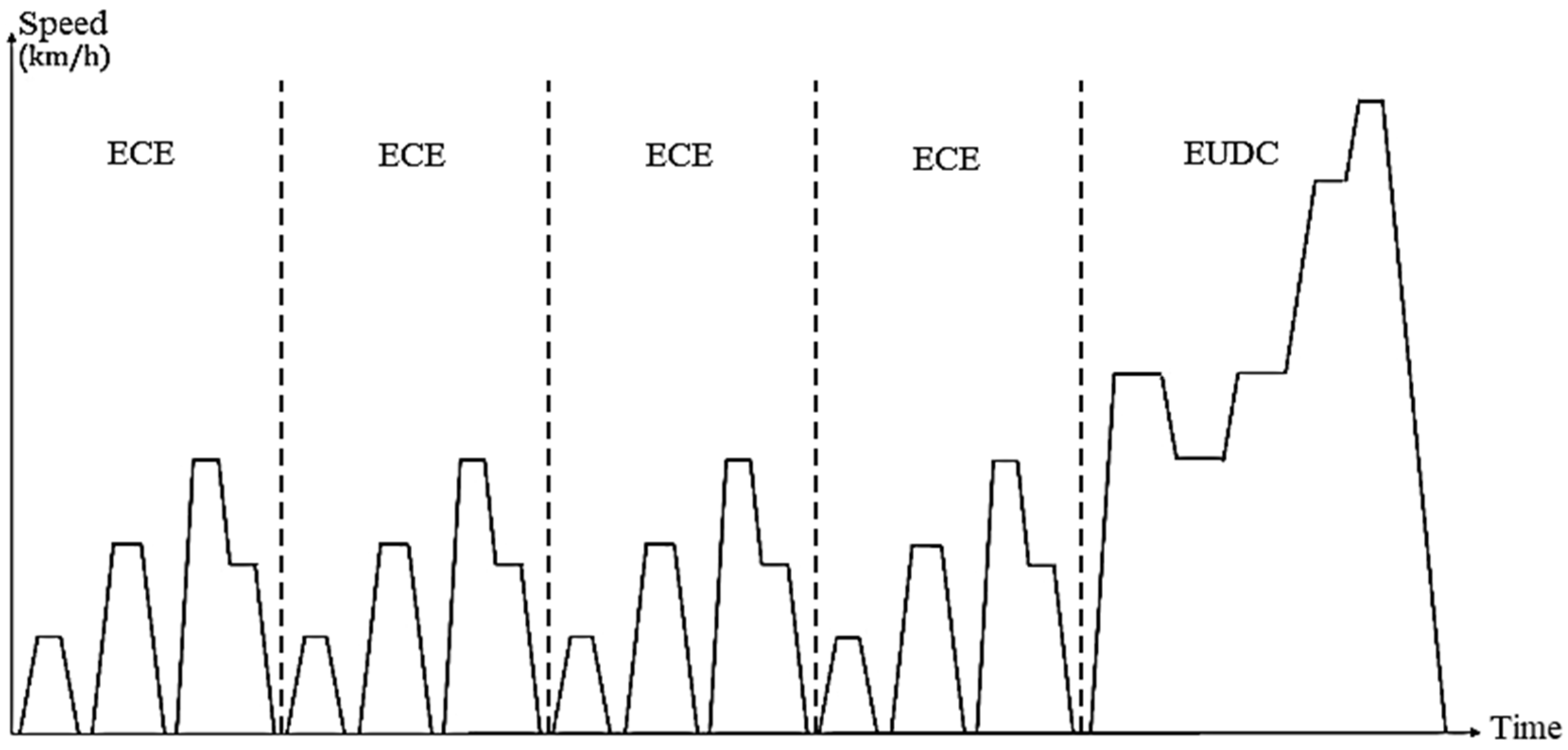
Like that of CVs, the typical driving state of an EV consists of starting, accelerating, constant speed, decelerating, and stopping, and the driving state transforms from one to another during travel. Previous work either assumed a constant speed of EVs, or a linear coefficient between energy consumption and distance, which ignores the changes in driving states. Therefore, in this work, we use a more realistic model based on the driving cycles with consideration of the factors of load, travel distance, and speed. The driving cycle of a vehicle presents the change in speed with the change in driving states. The New European Driving Cycle (NEDC), which is widely used to estimate EVs’ maximum driving range in China, includes two test cycles: that of the Economic Commission for Europe (ECE) and the Extra Urban Driving Cycle (EUDC). The driving cycles of ECE and EUDC are shown in Figure 1.

ECE tests an EV operating within a city for the first four cycles, whereas EUDC tests it in a suburban area for the last cycle. The EV in EUDC operates at a higher speed than that in ECE. The driving cycle shows the change in speed over time. During ECE, the vehicle first accelerates from rest before it reaches a constant speed and runs for a period, after which it decelerates to stop and then starts to repeat similar movements. By comparison, during EUDC, the vehicle accelerates from a standstill, then undergoes an acceleration and deceleration process with different change rates, before it finally stops.

When using EVs in urban distribution, there are three types of nodes in the network: (1) distribution center $N_D$; (2) customers $N_C$; and (3) recharging stations $N_R$. EVs depart from $N_D$ in suburban areas and visit $N_C$ in the city for delivery. They visit the recharging stations when necessary, and return to $N_D$ after completing the task. By comparison, the driving cycle of EVs driving from and returning to $N_D$ is similar to that of EUDC, whereas driving between $N_C$ and $N_R$ is similar to that of ECE. Therefore, we present the following driving conditions of EVs to further describe their driving cycles.

Condition A: EVs depart from a distribution center to the first customer, or EVs return to the distribution center from the last customer.

Under this condition, an EV first starts from a stationary position and accelerates at a uniform rate $a_{a1}$ until its speed reaches $v_{a1}$, then it decelerates to $v_{a2}$ at rate $a_{a2}$. Then, it accelerates again at rate $a_{a3}$ to speed $v_{a3}$, then travels at a constant speed $v_{a3}$ for some time, and finally decelerates to a full stop at rate $a_{a4}$. This driving cycle is named cycle A, as shown in Figure 2.

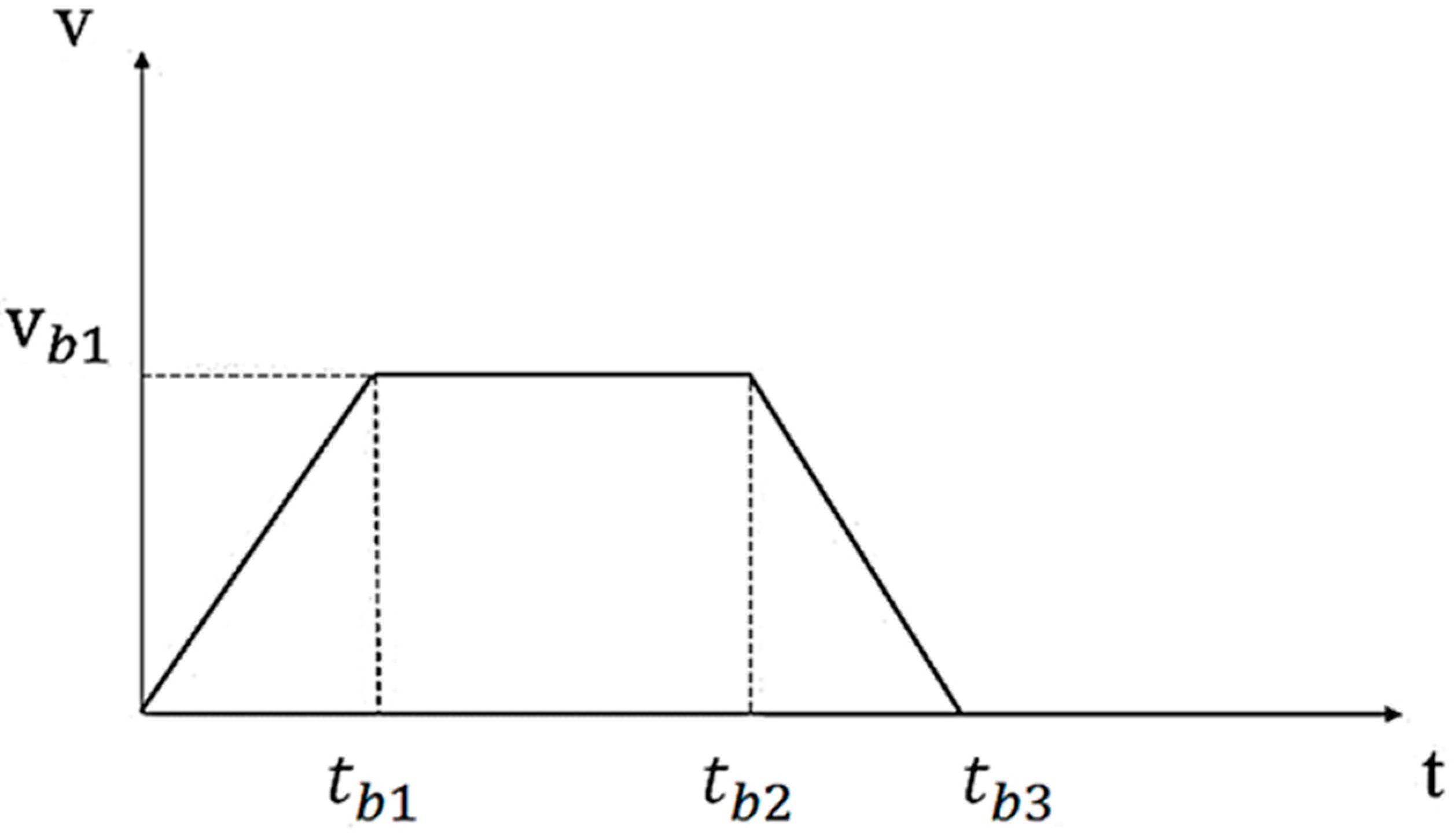
Condition B: During delivery, EVs travel between customer and customer, or between customer and recharging station.

Under condition B, the driving cycle of an EV is as follows: an EV starts from a stationary position at a customer or recharging station, then accelerates at a uniform rate $a_{b1}$ to speed $v_{b1}$ and maintains $v_{b1}$ for a period, after which it decelerates at rate $a_{b2}$ to a complete stop when it reaches the next customer or recharging station. This driving cycle B is shown in Figure 3.

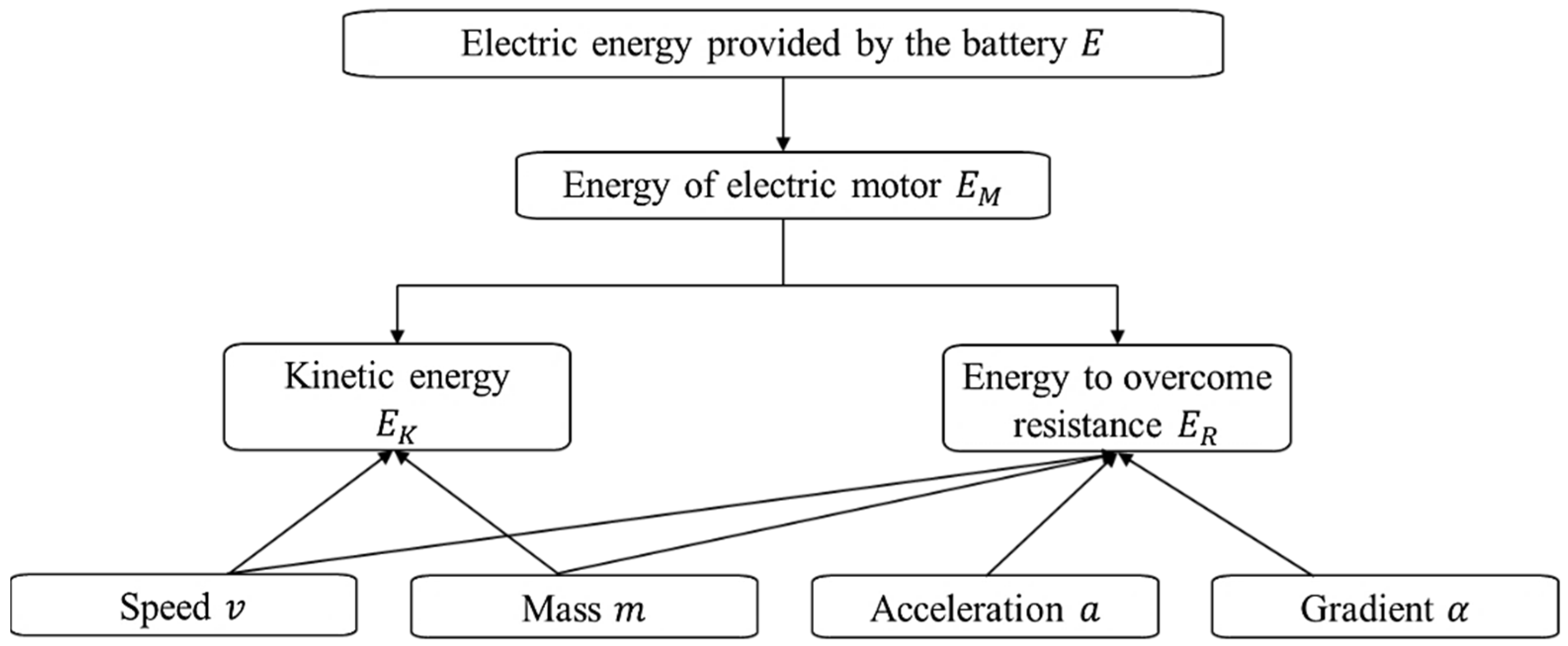
3.2. Energy Consumption Models of EVs Based on Different Driving Cycles

We develop the energy consumption models of an EV in a few steps, as shown in Figure 4. According to the kinetic energy theorem, the kinetic energy obtained by the vehicle should be equal to the work done by the vehicle’s combined external force, while the total external force is the difference between the vehicle’s traction and resistance. Therefore, during an EV’s driving process, both the kinetic energy $E_K$ and the energy consumed to overcome resistance $E_R$ come from the electric energy of the motor $E_M$:

$$E_M=E_K+E_R$$

(1)

$E_M$ is then translated into the electric energy $E$ provided by the battery, that is:

$$E=\frac{E_M}{\eta }$$

(2)

where $\eta$ is the efficiency of the electric motor.

Similar to combustion vehicles, EVs are influenced by four types of external forces during driving, namely, rolling resistance $F_f$, acceleration resistance $F_j$, slope resistance $F_g$, and air resistance $F_w$. Resistances are mainly determined by factors of vehicle mass, vehicle load, vehicle dimensions, engine properties, acceleration rate, speed, and gradient.

To present the equations of resistance, we use the notation shown in

Table 1. Notation to calculate resistance.

Notation	Definition
$\mathit{m}$	Mass of an EV in kilograms
$\mathit{g}$	Gravitational acceleration constant
$\mathit{\alpha }$	Gradient angle
$\mathit{f}$	Rolling friction coefficient
$\mathit{\delta }$	The conversion factor of vehicle rotation mass
$\mathit{v}$	Speed
${\mathit{\rho }}_{\mathit{a}}$	Air density
${\mathit{C}}_{\mathit{d}}$	Aerodynamic drag coefficient
${\mathit{A}}_{\mathit{f}}$	Vehicle frontal area

.

Then, the rolling resistance $F_f$, the acceleration resistance $F_j$, the air resistance $F_w$, and the slope resistance $F_g$ can be respectively determined as:

$$F_f=f\cdot m\cdot g$$

(3)

$$F_j=\delta \cdot m\cdot a$$

(4)

$$F_w=\frac{1}{2}\cdot {\rho }_a\cdot C_d\cdot A_f\cdot v^2$$

(5)

$$F_g=m\cdot g\cdot \mathit{sin}\alpha$$

(6)

In the following, the steps to build energy consumption models for driving cycles A and B are described in further detail. Let $d$ be the distance between any two nodes, and $s$ the distance an EV drives. We start with driving cycle B as it has fewer phases.

Driving cycle B, as shown in previous Figure 3, consists of three phases: first acceleration phase, second uniform motion phase, and, finally, the deceleration phase.

The first acceleration phase is from speed 0 to $v_{b1}$ during time 0 to $t_{b1}$, that is:

$$E_{B1}=\frac{E_K+E_R}{\eta }=\frac{\frac{1}{2}m{v}_{b1}^2+E_R}{\eta }$$

(7)

and:

$$E_R=F_f\cdot s_{b1}+F_j\cdot s_{b1}+F_g\cdot s_{b1}+F_w\cdot s_{w,b1}$$

(8)

where $s_{b1}$ is the distance the EV travels during this phase, while $s_{w,b1}$ is the distance traveled when facing air resistance.

Based on the law of uniform acceleration:

$$s_{b1}=\frac{1}{2}{a}_{b1}{t}_{b1}^2$$

(9)

the intensity of air resistance is changed by speed; then, based on the infinitesimal method:

$$F_w\cdot s_{w,b1}={\int }_0^{t_{b1}}\frac{1}{2}{\rho }_a{C}_d{A}_f{v}^2\cdot vdt$$

(10)

This converts into:

$$F_w\cdot s_{w,b1}=\frac{1}{8}{\rho }_a{C}_d{A}_f{a}_{b1}^3{t}_{b1}^4$$

(11)

Therefore:

$$E_R=fmg\cdot \frac{1}{2}{a}_{b1}{t}_{b1}^2+\delta m{a}_{b1}\cdot \frac{1}{2}{a}_{b1}{t}_{b1}^2+mgsin\left(\alpha \right)\cdot \frac{1}{2}{a}_{b1}{t}_{b1}^2+\frac{1}{8}{\rho }_a{C}_d{A}_f{a}_{b1}^3{t}_{b1}^4$$

(12)

The battery energy consumed during the acceleration phase of cycle B, $E_{B1}$, is then calculated as below:

$$E_{B1}=\frac{\frac{1}{2}m{v}_{b1}^2+\frac{1}{2}m\left(gf+\delta a_{b1}+g\mathit{sin}\alpha \right)a_{b1}{t}_{b1}^2+\frac{1}{8}{\rho }_a{C}_d{A}_f{a}_{b1}^3{t}_{b1}^4}{\eta }$$

(13)

In the second uniform motion phase, the acceleration resistance $F_j$ is 0 due to 0 acceleration and constant speed, while air resistance $F_w$ is constant. The battery energy consumed during this phase of cycle B, $E_{B2}$, is determined as:

$$\begin{array}{l}{E}_{B2}=\frac{F_f+F_g+F_w\cdot s_{b2}}{\eta }\\ =\frac{\left(mgf+mgsin\alpha +\frac{1}{2}{\rho }_a{C}_d{A}_f{v}_{b1}^2\right)\cdot v_{b1}\left(t_{b2}-t_{b1}\right)}{\eta }\end{array}$$

(14)

In the last phase of deceleration, regardless of energy recovery, all the kinetic energy is converted into work to overcome the resistance, so the battery output power is 0, and the battery does not consume energy; that is, $E_{B3}=0$.

Based on the law of uniform acceleration and uniform deceleration:

$$t_{b1}=\frac{v_{b1}}{a_{b1}}$$

(15)

$$s_{b1}=\frac{v_{b1}^2}{2a_{b1}}$$

(16)

$$s_{b3}=\frac{v_{b1}^2}{2a_{b2}}$$

(17)

$t_{b1}$ and $s_{b1}$ are the driving time and distance in the acceleration phase, respectively, and $s_{b3}$ is the driving distance in the deceleration phase.

With known distance $d$ between any two nodes, the distance traveled in the uniform motion phase is calculated as:

$$s_{b2}=d-\frac{v_{b1}^2}{2a_{b1}}-\frac{v_{b1}^2}{2a_{b2}}$$

(18)

Inserting Equations (15)–(18) into Equations (13) and (14), we have:

$$E_{B1}=\frac{\frac{1}{2}m{v}_{b1}^2+\frac{v_{b1}^2}{2a_{b1}}m\left(gf+\delta a_{b1}+g\mathit{sin}\alpha \right)+\frac{v_{b1}^4}{8a_{b1}}{\rho }_a{C}_d{A}_f}{\eta }$$

(19)

$$E_{B2}=\frac{\left(\mathit{mgf}+\mathit{mgsin}\alpha +\frac{1}{2}{\rho }_a{C}_d{A}_f{v}_{b1}^2\right)\cdot \left(d-\frac{v_{b1}^2}{2a_{b1}}-\frac{v_{b1}^2}{2a_{b2}}\right)}{\eta }$$

(20)

Therefore, the total battery energy consumed during the entire driving cycle B is determined as:

$$E^B=E_{B1}+E_{B2}$$

(21)

Driving cycle A, as in Figure 2, has five sequential phases: first acceleration, first deceleration, second acceleration, uniform motion, and second deceleration phase. Similar to the case of cycle B, in acceleration phases, the electric energy is converted into kinetic energy and the energy to overcome external resistance; in the uniform motion phase, the energy from the battery is used to overcome resistance; and in deceleration phases, the battery does not consume any energy.

In the first acceleration phase from time 0 to $t_{a1}$, the battery energy consumed is:

$$E_{A1}=\frac{\frac{1}{2}m{v}_{a1}^2+\frac{v_{a1}^2}{2a_{a1}}m\left(gf+\delta a_{a1}+g\mathit{sin}\alpha \right)+\frac{v_{a1}^4}{8a_{a1}}{\rho }_a{C}_d{A}_f}{\eta }$$

(22)

From time $t_{a2}$ to $t_{a3}$ of the second acceleration phase, based on the kinetic energy theorem:

$$\frac{1}{2}m{v}_{a3}^2-\frac{1}{2}m{v}_{a2}^2=\eta E_{A3}-E_R$$

(23)

Then,

$$E_{A3}=\frac{\frac{1}{2}m\left(v_{a3}^2-v_{a2}^2\right)+\frac{v_{a3}^2-v_{a2}^2}{2a_{a3}}m\left(gf+\delta a_{a1}+g\mathit{sin}\alpha \right)+E_{F_w}}{\eta }$$

(24)

with:

$$E_{F_w}=\frac{{\rho }_a{C}_d{A}_f}{8a_{a3}}\left[{\left(v_{a2}+a_{a3}{t}_{a3}\right)}^4-{\left(v_{a2}+a_{a3}{t}_{a2}\right)}^4\right]$$

(25)

Based on the law of uniform acceleration and uniform deceleration:

$$t_{a1}=\frac{v_{a1}}{a_{a1}}$$

(26)

$$t_{a2}=t_{a1}+\frac{v_{a1}-v_{a2}}{a_{a2}}$$

(27)

$$t_{a3}=t_{a2}+\frac{v_{a3}-v_{a2}}{a_{a3}}$$

(28)

Insert $t_{a1}$, $t_{a2}$, and $t_{a3}$ into Equation (25); after simplification, we obtain:

$$\begin{array}{c}{E}_{F_w}=\frac{{\rho }_a{C}_d{A}_f}{8a_{a3}}\{{[v_{a2}+\frac{v_{a1}{a}_{a2}{a}_{a3}+a_{a1}{a}_{a3}\left(v_{a1}-v_{a2}\right)+a_{a1}{a}_{a2}\left(v_{a3}-v_{a2}\right)}{a_{a1}{a}_{a2}}]}^4\\ -{[v_{a2}+\frac{v_{a1}{a}_{a2}{a}_{a3}+a_{a1}{a}_{a3}\left(v_{a1}-v_{a2}\right)}{a_{a1}{a}_{a2}}]}^4\}\end{array}$$

(29)

In the uniform motion phase, from time $t_{a3}$ to $t_{a4}$, which is similar to that in cycle B, the battery energy in this phase of cycle A is calculated using:

$$\begin{array}{c}{E}_{A4}=\\ \frac{\left(mgf+mg\mathit{sin}\alpha +\frac{1}{2}{\rho }_a{C}_d{A}_f{v}_{a3}^2\right)\cdot \left(d-\frac{v_{a1}^2}{2a_{a1}}-\frac{v_{a1}^2-v_{a2}^2}{2a_{a2}}-\frac{v_{a3}^2-v_{a2}^2}{2a_{a3}}-\frac{v_{a3}^2}{2a_{a4}}\right)}{\eta }\end{array}$$

(30)

Since the other two phases are the deceleration process, $E_{A2}=0$, and $E_{A5}=0$. Therefore, the total battery energy consumed during driving cycle A is determined as:

$$E^A=E_{A1}+E_{A3}+E_{A4}$$

(31)

4. The Electric Vehicle Routing Problem with Time Windows Based on Driving Cycles (EVRPTW-DC)

4.1. Formulation of EVRPTW-DC

The electric vehicle routing problem in our work is constructed using the energy consumption models established in Section 3, also with consideration of customer time windows, the safe battery level, and vehicle load capacity. We define EVRPTW-DC with the following assumptions:

• Only one distribution center exists and all EVs depart from the distribution center at the same time with a full battery, and return to the same distribution center after completing the delivery tasks;
• EVs are homogeneous;
• When visiting a recharging station, an EV is always recharged to full battery capacity;
• Only delivery tasks for a customer are considered, i.e., no pickup tasks;
• A customer must be visited only once, and by only one vehicle;
• The locations of the distribution center, customers, and recharging stations, and the demands of customers, are known;
• The number of chargers is sufficient at any recharging station, and an EV can be serviced whenever it arrives.

With the above assumptions, we now present the notation of our model in

Table 2. Notation of variables and parameters in the EVRPTW-DC model.

Sets
$N$	Set of all nodes
$N_0$	Distribution center
$N_C$	Set of customers
$N_R$	Set of recharging stations
$K$	Set of EVs
Parameters
$T_{lim}$	The maximum time span of a delivery route, in hour units
$Q$	The maximum battery level of an EV, in $\mathrm{kW}·\mathrm{h}$
$Q_{low}$	The lowest battery level of an EV, in $\mathrm{kW}·\mathrm{h}$
$r$	Recharging rate at a charger, in kW
$\varphi$	Unit price of recharging, in $\mathrm{Yuan}/(\mathrm{kW}·\mathrm{h})$
$M$	Number of available EVs at the distribution center
$W$	The maximum load of an EV, in kg
${\lambda }_1$	Unit cost of a vehicle arriving before the time window, in Yuan/h
${\lambda }_2$	Unit cost of a vehicle arriving after the time window, in Yuan/h
$v_{ai}$	The speed of an EV in driving cycle A, $i=1,2,3$$,\mathrm{in}\mathrm{m}/\mathrm{s}$
$a_{ai}$	The acceleration of an EV in driving cycle A, $i=1,2,3,4$$,\mathrm{in}\mathrm{m}/{\mathrm{s}}^2$
$v_{bi}$	The speed of an EV in driving cycle B, $i=1,2,3,4$$,\mathrm{in}\mathrm{m}/\mathrm{s}$
$a_{bi}$	The acceleration of an EV in driving cycle B, $i=1,2,$$\mathrm{in}\mathrm{m}/{\mathrm{s}}^2$
$c_1$	Unit cost of traveled distance, in Yuan/km
$c_2$	Fixed cost for recharging
$q_i$	The demand of node $i$$,i\in N_C$
${\mu }_i$	Earliest start of service at node $i$$,i\in N_C$
$l_i$	Latest start of service at node $i$$,i\in N_C$
$d_{ij}$	Distance between node $i$ and $j$, $i,j\in N$
$t_{ijk}$	Travel time of vehicle $k$ between node $i$ and $j$$,i,j\in N, k\in K$
$E_{ijk}$	Battery energy consumption of vehicle $k$ between node i and j, $i,j\in N$, $k\in K$; and is calculated by Equations (21) and (31) depending on driving cycle
Variables
$t_{ik}^a$	Time of arrival of vehicle $k$ at node $i$, $i\in N, k\in K$
$t_{ik}^l$	Time of arrival of vehicle $k$ at node $i$, $,i\in N, k\in K$
$t_{ik}^s$	The service time or recharging time of vehicle $k$ at node $i$$,i\in N, k\in K$
$t_{ik}^w$	The waiting time of vehicle $k$ at node $i$, $i\in N, k\in K$
$p_{ik}^a$	Battery level of vehicle $k$ when arriving node $,i\in N, k\in K$
$p_{ik}^l$	Battery level of vehicle $k$ when leaving node $i$, $i\in N, k\in K$
$w_{ik}$	Load of vehicle $k$ when arriving node $i$, $i\in N, k\in K$
$E_{ijk}$	Battery energy consumption of vehicle $k$ between node $i$ and $j$, $i,j\in N$, $k\in K$; and is calculated by Equations (21) and (31) depending on driving cycle
$x_{ijk}$	Binary decision variable indicating if vehicle $k$ travels from node $i$ to node $j$$,i,j\in N, k\in K$

.

The objective for EVRPTW-DC is to minimize the total costs of distance, recharging, and time window punishment.

(1)

Cost of traveled distance C_d:

$$C_d=c_1{\displaystyle \sum }_{i\in N}{\displaystyle \sum }_{j\in N}{\displaystyle \sum }_{k\in K}{x}_{ijk}{d}_{ij}$$

(32)

(2)

Cost of recharging C_r:

$$C_r=\left[c_2+\varphi \left(Q-p_{jk}^a\right)\right]{\displaystyle \sum }_{i\in N}{\displaystyle \sum }_{j\in N_R}{\displaystyle \sum }_{k\in K}{x}_{ijk}$$

(33)

$C_r$ consists of two components: the fixed cost for using a recharging facility, and the variable cost depending on the amount of recharged energy. To linearize $C_r$, we introduce new nonnegative variables $y_{ijk}$.

Let $y_{ijk}=p_{jk}^a{x}_{ijk}$, and, with the below constraints:

$$y_{ijk}\le Q{x}_{ijk}$$

(34)

$$y_{ijk}\le p_{jk}^a$$

(35)

$$y_{ijk}\ge p_{jk}^a-Q(1-x_{ijk})$$

(36)

Equation (33) can be transformed into a linear formation as:

$$C_r=c_2{\displaystyle \sum }_{i\in N}{\displaystyle \sum }_{j\in N_R}{\displaystyle \sum }_{k\in K}{x}_{ijk}+\varphi Q{\displaystyle \sum }_{i\in N}{\displaystyle \sum }_{j\in N_R}{\displaystyle \sum }_{k\in K}{x}_{ijk}-\varphi {\displaystyle \sum }_{i\in N}{\displaystyle \sum }_{j\in N_R}{\displaystyle \sum }_{k\in K}{y}_{ijk}$$

(37)

(3)

Cost of time window punishment C_t:

$$C_t={\displaystyle \sum }_{i\in N_C}{\displaystyle \sum }_{k\in K}f\left(t_{ik}^a\right)$$

(38)

with:

$$f\left(t_{ik}^a\right)=\{\begin{array}{ccc}{\lambda }_1\left(u_i-t_{ik}^a\right)& & t_{ik}^a<u_i\\ 0& & u_i\le t_{ik}^a\le l_i\\ {\lambda }_2\left(t_{ik}^a-l_i\right)& & l_i<t_{ik}^a\end{array}, \forall i\in N_C,k\in K$$

(39)

To linearize $f\left(t_{ik}^a\right)$, we introduce new variables ${\epsilon }_{ik}$ and ${\xi }_{\mathit{ik}}$ for $i\in N_C,k\in K$, which are defined as:

$${\epsilon }_{ik}=max\left({\lambda }_1\left(u_i-t_{ik}^a\right),0\right)$$

(40)

$${\xi }_{\mathit{ik}}=max\left(0,{\lambda }_2\left(t_{ik}^a-l_i\right)\right)$$

(41)

Then, $f\left(t_{ik}^a\right)$ is replaced by:

$$f\left(t_{ik}^a\right)={\epsilon }_{ik}+{\xi }_{\mathit{ik}}$$

(42)

and Equation (38) is transformed into:

$$C_t={\displaystyle \sum }_{i\in N_C}{\displaystyle \sum }_{k\in K}({\epsilon }_{ik}+{\xi }_{ik})$$

(43)

Therefore, the objective function is presented as:

$$\mathrm{MIN}C=C_d+C_r+C_t$$

(44)

The constraints of EVRPTW-DC are as follows:

$${\displaystyle \sum }_{k\in K}{\displaystyle \sum }_{i\in N_C, i\ne j}{x}_{ijk}=1 \forall j\in N$$

(45)

$${\displaystyle \sum }_{i\in N, i\ne j}{x}_{ijk}={\displaystyle \sum }_{s\in N, j\ne s}{x}_{jsk} \forall k\in K, j\in N$$

(46)

$${\displaystyle \sum }_{k\in K}{\displaystyle \sum }_{j\in N_C}{x}_{0jk}\le M$$

(47)

$${\displaystyle \sum }_{j\in N}{x}_{0jk}=1 \forall k\in K$$

(48)

$${\displaystyle \sum }_{i\in N}{x}_{i0k}=1 \forall k\in K$$

(49)

$$0\le w_{0k}\le W \forall k\in K$$

(50)

$$\begin{array}{c}0\le w_{jk}\le w_{ik}-q_i{x}_{ijk}+W\left(1-x_{ijk}\right)\hfill \\ \forall i\in N,\forall j\in \left\{N_C\cup N_R\right\}, i\ne j,\forall k\in K\end{array}$$

(51)

$$p_{ik}^l=Q \forall i\in \left\{N_0\cup N_R\right\},\forall k\in K$$

(52)

$$p_{ik}^a=p_{ik}^l \forall i\in N_C,\forall k\in K$$

(53)

$$Q_{low}\le p_{ik}^a,p_{ik}^l\le Q \forall i\in N,\forall k\in K$$

(54)

$$p_{jk}^a\le p_{ik}^l-E_{ijk}{x}_{ijk}+Q\left(1-x_{ijk}\right) \forall i,j\in N,i\ne j,\forall k\in K$$

(55)

$$p_{ik}^l\ge \min \left\{E_{i0k}{x}_{i0k},E_{ijk}{x}_{ijk}\right\} \forall i\in N_C,j\in N_R,\forall k\in K$$

(56)

$$t_{0k}^l=0 \forall k\in K$$

(57)

$$0\le t_{ik}^a,t_{ik}^l\le T_{\mathit{lim}} \forall i\in N,\forall k\in K$$

(58)

$$t_{ik}^l+t_{i0k}\le T_{lim} \forall i\in \left\{N_C\cup N_R\right\},\forall k\in K$$

(59)

$$t_{jk}^a\ge t_{ik}^l+t_{ijk}{x}_{ijk}-T_{lim}\left(1-x_{ijk}\right) \forall i,j\in N,i\ne j,\forall k\in K$$

(60)

$$t_{ik}^l=t_{ik}^a+t_{ik}^s+t_{ik}^w \forall i\in \left\{N_C\cup N_R\right\},\forall k\in K$$

(61)

$$t_{ik}^w=max\{0,\left(u_i-t_{ik}^a\right)\} \forall i\in N_C,\forall k\in K$$

(62)

$$t_{ik}^s=\{\begin{array}{cc}\theta & \forall i\in N_C,\forall k\in K\\ \frac{Q-p_{ik}^a}{r}& \forall i\in N_R,\forall k\in K\end{array}$$

(63)

$$t_{ijk}=\left\{\begin{array}{cc}\begin{array}{c}\frac{v_{a1}}{a_{a1}}+\frac{v_{a1}-v_{a2}}{a_{a2}}+\frac{v_{a3}-v_{a2}}{a_{a3}}+\frac{v_{a3}}{a_{a4}}\\ +\frac{d_{ij}-\frac{v_{a1}^2}{2a_{a1}}-\frac{v_{a1}^2-v_{a2}^2}{2a_{a2}}-\frac{v_{a3}^2-v_{a2}^2}{2a_{a3}}-\frac{v_{a3}^2}{2a_{a4}}}{v_{a3}}\end{array}& \begin{array}{c}i=0, \forall j\in \{N_C\cup N_R\}, or\\ \forall i\in \{N_C\cup N_R\}, j=0 \forall k\in K\end{array}\\ \frac{v_{b1}}{a_{b1}}+\frac{v_{b1}}{a_{b2}}+\frac{d_{ij}-\frac{v_{b1}^2}{2a_{b1}}-\frac{v_{b1}^2}{2a_{b2}}}{v_{b1}}& \begin{array}{c}\forall i,j\in \{N_C\cup N_R\}i\ne j,\\ \forall k\in K\end{array}\end{array}\right.$$

(64)

Constraint (45) ensures that each customer must be visited exactly once. The Flow Constraint (46) guarantees for each node that the incoming flow is equal to the outgoing flow for each vehicle. Constraint (47) ensures that the number of employed vehicles does not exceed the number of available vehicles. Constraints (48) and (49) ensure each vehicle departs from and returns to the distribution center. Constraint (50) restricts the initial load to the maximum load capacity of a vehicle, and Constraint (51) enforces the fulfillment of demand at customer nodes. Constraint (52) ensures the battery level is at the maximum capacity when leaving the distribution center and recharging stations. The battery level maintains the same level at a customer node, as presented in Constraint (53). Constraint (54) ensures the battery level is within the range of minimum and maximum levels. Constraint (55) sets the battery level at a node succeeding a previous node according to the energy consumption models introduced in Section 3. Constraint (56) guarantees that the battery level when leaving a customer node should at least allow the vehicle to either return to the distribution center or travel to the closest recharging station.

All vehicles depart from the distribution center at time 0, as constrained in (57). Constraint (58) ensures the arrival and departure time at any node be within the maximum time span, while Constraint (59) ensures the time any vehicle returns to the distribution center is also within the maximum time span. Constraint (60) links the arrival time at a node with the departure time from the previous node. Constraint (61) illustrates that the departure time from a node is composed of arrival time, service time, and waiting time at this node. Constraint (62) calculates the waiting time at a customer node if the vehicle arrives earlier than the earliest service time. The service time at a node is either constant for a customer node, or the time required for recharging to full battery capacity at a recharging station, as presented in Constraint (63). Constraint (64) calculates the driving time between any two nodes, depending on driving cycles A and B in Section 3.

4.2. EVRPTW with Linear Energy Consumption (L-EVRPTW)

Most of the previous works on EVRP assumed energy consumption to be a linear function of the traveled distance, which is less realistic compared to our proposed EVRPTW-DC. To conduct comparative analysis in a later section, here we present a brief introduction of EVRPTW with linear energy consumption, denoted as L-EVRPTW.

Unlike EVRPTW-DC, L-EVRPTW has assumptions of constant speed during driving, and the energy consumption is linearly related to traveled distance only, without considering the impacts of speed and load. In addition to the notations in previous Table 2, $v$ represents the constant speed of EVs, and $\zeta$ is the energy consumption rate, which is also constant. The battery energy consumed between two nodes $i$ and $j$ with distance $d_{ij}$ can then be calculated by the below formula:

$$E_{ij}=\zeta ·d_{ij}, \hspace{1em} \forall i,j\in N,k\in K$$

(65)

The travel time is determined as:

$$t_{ijk}=\frac{d_{ij}}{v}, \forall i,j\in N,k\in K$$

(66)

The remainder of the constraints and objective function of L-EVRPTW are the same as EVRPTW-DC.

5. Adaptive Particle Swarm Optimization Algorithm for Solving EVRPTW-DC

This section details the adaptive particle swarm optimization (PSO) algorithm for our proposed EVRPTW-DC model. PSO was first introduced by Kennedy and Eberhart in 1995, and simulated the cooperation mechanism in foraging behavior in a swarm of birds and fish to search for the optimal solution [25].

In standard PSO, each particle has two attributes: position and velocity. The swarm searches for the best solution in an $n$-dimensional space. The position of a particle represents a solution and is adjusted by velocity to search for new solutions. The particle records the best position, $pbest$, it reached, and the best position experienced by the entire swarm, $gbest$, is also recorded [26].

In each iteration, the velocities $\overrightarrow{v}$ and positions $\overrightarrow{x}$ of the particles are updated by the following rules:

$${\overrightarrow{v}}_{id}^{t+1}=\omega {\overrightarrow{v}}_{id}^t+{\phi }_1{\gamma }_1\left(pbes{t}_{id}^t-{\overrightarrow{x}}_{id}^t\right)+{\phi }_2{\gamma }_2\left(gbes{t}_{id}^t-{\overrightarrow{x}}_{id}^t\right)$$

(67)

$${\overrightarrow{x}}_{id}^{t+1}={\overrightarrow{x}}_{id}^t+{\overrightarrow{v}}_{id}^{t+1}$$

(68)

where $pbest$ is the best solution a particle has found and $gbest$ is the best solution the swarm has found. $\omega$, ${\phi }_1$, and ${\phi }_2$ are important parameters for PSO. $\omega$ is the parameter called inertia weight, which serves as a memory of particle velocity from the last iteration, preventing the particle from drastically changing direction. ${\phi }_1$ and ${\phi }_2$ are acceleration coefficients, affecting the self-learning ability and social-learning ability of the particle, respectively. ${\gamma }_1$ and ${\gamma }_2$ are random numbers within 0 to 1.

The proposed adaptive PSO for EVRPTW-DC consists of similar attributes and parameters but with additional steps to check battery constraints as shown in Figure 5.

5.1. Particles Coding and Decoding

The solutions of EVRPTW-DC represented by particles are encoded by two vectors, $X_v$ and $X_r$, for vehicle and service order, respectively [27]. For illustration, the problem has a total of nine customers and three available vehicles, and a delivery plan is presented in

Table 3. Example of particle coding.

Customers	1	2	3	4	5	6	7	8	9
Vector of Vehicles	1	2	3	1	3	2	1	1	3
Vector of Service Orders	3	2	3	1	1	1	4	2	2

.

The vector of vehicles indicates the IDs of vehicles serving each customer, indicating that customers 1, 4, 7, and 8 are visited by vehicle 1; customers 2 and 6 are visited by vehicle 2; and the rest of the customers are visited by vehicle 3. The vector of service orders indicates the sequence of visiting each customer by a vehicle, which is the path of the vehicle. The vector of service orders indicates that vehicle 1 first visits customer 4, secondly customer 8, then customer 1, and finally customer 7. Similarly, we can decode the paths for vehicles 2 and 3, as listed in

Table 4. Example of decoded paths.

Vehicle 1	4 → 8 → 1 → 7
Vehicle 2	6 → 2
Vehicle 3	5 → 9 → 3

.

Note that, due to the randomness of initialization and the iterative process, there may be solutions that do not meet the model constraints during the iterations, e.g., the same customer appearing on the delivery paths of multiple vehicles, and those solutions need to be eliminated after decoding.

5.2. Settings of Adaptive PSO

Similar to standard PSO, particles of adaptive PSO are updated in each iteration. As mentioned in Section 5.1, a particle is encoded by two vectors $X_v$ and $X_r$. Let $V_v$ and $V_r$ be the velocities of $X_v$ and $X_r$, respectively. The velocities and positions in iteration $i+1$ are updated by the following equations:

$${\overrightarrow{V}}_v^{i+1}=\omega {\overrightarrow{V}}_v^i+{\phi }_1{\gamma }_1\left(pbes{t}_{X_v}^i-{\overrightarrow{X}}_v^i\right)+{\phi }_2{\gamma }_2\left(gbes{t}_{X_v}^i-{\overrightarrow{X}}_v^i\right)$$

(69)

$${\overrightarrow{X}}_v^{i+1}={\overrightarrow{X}}_v^i+{\overrightarrow{V}}_v^{i+1}$$

(70)

$${\overrightarrow{V}}_r^{i+1}=\omega {\overrightarrow{V}}_r^i+{\phi }_1{\gamma }_1\left(pbes{t}_{X_r}^i-{\overrightarrow{X}}_r^i\right)+{\phi }_2{\gamma }_2\left(gbes{t}_{X_r}^i-{\overrightarrow{X}}_r^i\right)$$

(71)

$${\overrightarrow{X}}_r^{i+1}={\overrightarrow{X}}_r^i+{\overrightarrow{V}}_r^{i+1}$$

(72)

The value of $\omega$ has a significant influence on the global search ability and local search ability of PSO algorithm. According to the research by Zhao and Deng [28], choosing a larger $\omega$ in the preliminary stage can make the algorithm have a stronger global search ability, whereas in the later stage, a smaller $\omega$ can improve the convergence speed of the algorithm. Therefore, in the adaptive PSO for our problem, we adopt a linearly decreasing selection strategy for $\omega$ to improve the searching ability and convergence speed of the algorithm, and update its value by the following formula [29]:

$$\omega ={\omega }_{max}-\left({\omega }_{max}-{\omega }_{min}\right)\ast \left(\frac{{{\rm I}}_{current}}{{{\rm I}}_{max}}\right)$$

(73)

where ${{\rm I}}_{current}$ is the current iteration number and ${{\rm I}}_{max}$ is the maximum number of iterations. ${\omega }_{max}$ and ${\omega }_{min}$ are set to be 0.9 and 0.4, respectively. ${\phi }_1$ and ${\phi }_2$ are both set to be 1.494 based on Clrec’s research [30].

6. Case Study

Company J is an e-commerce enterprise that has its own distribution network. The cases in this section are constructed based on the actual distribution network of company J. The warehouse of company J serving the greater Xi’an area is selected as the distribution center $N_0$ and a few EVs are used to perform daily delivery tasks. The customer set $N_C$ consist of outlets within the city of Xi’an, with known locations, demands, and time windows. In addition, public recharging stations are selected as the charging facilities $N_R$ in the distribution network. The locations of facilities and the recharging rate are provided. Experiments are then conducted on three different scales of distribution network, with the same distribution center but a different number of customer nodes and maximum available EVs, as listed in

Table 5. Settings of three scenarios.

Number of	Distribution Center	Customer Nodes	Recharging Stations	Maximum Available EVs
Scenario 1	1	25	5	6
Scenario 2	1	30	5	8
Scenario 3	1	35	5	10

. Five recharging stations with the same unit charging rate and cost are selected for each scenario, but their locations may vary from scenario to scenario. Figure 6 shows the distribution networks of each scenario, including the distribution center, customers, and recharging stations.

6.1. Experimental Environment and Parameter Settings

There are various types of EVs on the market, with different load capacities and battery capacities. We compared the available EVs for logistics and selected five for experiments that have the listed attributes in

Table 6. Attributes of EVs.

Type	Mass $\left(\mathbf{k}\mathbf{g}\right)$	Max Load $\left(\mathbf{k}\mathbf{g}\right)$	Max Battery $(\mathbf{k}\mathbf{W}·\mathbf{h})$	Price (YUAN)
Type 1	3150	1215	96.77	158K
Type 2	2995	1305	87.20	239.8K
Type 3	4050	3105	96.76	217.8K
Type 4	2990	1310	103.42	240.5K
Type 5	3110	1265	83.20	324.8K

. Note that Company J adopted Type 4 EVs for daily delivery tasks to align with government policy and development.

Table 7. Parameters of driving resistance.

Parameters	Value
$g$	$9.8\mathrm{m}/{\mathrm{s}}^2$
$f$	0.01 [31]
$\delta$	1.14
$sin\alpha$	0.05
$C_d$	0.7 [32]
${\rho }_a$	$1.2 \mathrm{kg}/{\mathrm{m}}^3$ [32]
$A_f$	$5{\mathrm{m}}^2$

lists the values of parameters to calculate the driving resistance, and

Table 8. Parameters of driving cycles.

Driving Cycle	Parameters	Value
A	$v_{a1}$	$63 \mathrm{km}/\mathrm{h}$
	$v_{a2}$	$54 \mathrm{km}/\mathrm{h}$
	$v_{a3}$	$72 \mathrm{km}/\mathrm{h}$
	$a_{a1}$	$0.9 \mathrm{m}/{\mathrm{s}}^2$ [33]
	$a_{a2}$	$1.5 \mathrm{m}/{\mathrm{s}}^2$ [33]
	$a_{a3}$	$1 \mathrm{m}/{\mathrm{s}}^2$ [33]
	$a_{a4}$	$2 \mathrm{m}/{\mathrm{s}}^2$ [33]
B	$v_{b1}$	$36 \mathrm{km}/\mathrm{h}$
	$a_{b1}$	$0.9 \mathrm{m}/{\mathrm{s}}^2$ [33]
	$a_{b2}$	$1.5 \mathrm{m}/{\mathrm{s}}^2$ [33]

presents the values of speed and acceleration.

According to operational data of Company J, the average speed of vehicles during the overall route is between 30 and 40 km/h, while the driving speed in the suburban area differs from that within the city. Therefore, based on actual operational data and speed limits, the detailed speed and acceleration settings of driving cycles A and B are listed in Table 8.

The remainder of the parameters in the EVRPTW-DC model, such as unit distance cost, punishment of time window violation, recharging rate, and unit recharging cost, are presented in

Table 9. Other parameters of EVRPTW-DC.

Parameters	Definition	Value
$Q_0$	Safe battery level (20% of Max Battery)	$20.68\mathrm{kW}·\mathrm{h}$
${\lambda }_1$	Unit cost of vehicle arriving before time window	$3.6\mathrm{Yuan}/\mathrm{h}$
${\lambda }_2$	Unit cost of vehicle arriving after time window	$18\mathrm{Yuan}/\mathrm{h}$
$c_1$	Unit distance cost	$0.4\mathrm{Yuan}/\mathrm{km}$ [34]
$r$	Recharging rate	$60\mathrm{kW}$
$\varphi$	Unit recharging cost	$1.2\mathrm{Yuan}/\left(\mathrm{kW}·\mathrm{h}\right)$
$T_{lim}$	Maximum time span of a delivery route	$10\mathrm{h}$

, and

Table 10. Parameters of L-EVRPTW.

Parameters	Definition	Value
$\zeta$	Energy consumption rate	$1.03\mathrm{kW}·\mathrm{h}/\mathrm{km}$ [35]
$v$	Average speed	$35\mathrm{km}/\mathrm{h}$

provides the distinctive parameters, the energy consumption rate $\zeta$, and average speed $v$, for the L-EVRPTW model. The remaining experimental parameters listed in

Table 11. Parameters of PSO algorithm.

Parameters	Definition	Value
Num	Particle size	50
maxgen	Maximum number of iterations	200
${\phi }_1$	Learning coefficient 1	1.494
${\phi }_2$	Learning coefficient 2	1.494
${\omega }_{min}$	Minimum inertia coefficient	0.4
${\omega }_{max}$	Maximum inertia coefficient	0.9

are for the PSO algorithm.

6.2. Results and Analysis

6.2.1. Solutions of EVRPTW-DC and L-EVRPTW

Based on the scenarios and settings described earlier, we used MATLAB and Statistics Toolbox Release 2014a (The MathWorks, Inc., Natick, Massachusetts, United States) to build the PSO algorithm to solve the EVRPTW-DC and L-EVRPTW models, and the program was run on a desktop operating on Windows 10, with an Intel Core i5-7200U, 2.5 GHz processor, and 8 GB RAM. For each case, we conducted 20 individual tests and selected the best solution obtained among these tests to be the optimal solution achieved by our algorithm, which is presented in the following section.

We solved for EVRPTW-DC and L-EVRPTW individually. It is shown in Figure 7 and Figure 8 that our PSO algorithm is capable of solving scenarios with up to 35 customers. The number of iterations to obtain the optimum of EVRPTW-DC is similar to that of L-EVRPTW, and the number of iterations to obtain the optimum rises when the number of customers increases in both models. The optimal delivery paths are provided in

Table 12. Optimal delivery paths for EVRPTW-DC.

Vehicle	No.	Path
Scenario 1	1	0—1—2—0
	2	0—24—6—3—15—14—0
	3	0—22—4—0
	4	0—10—11—17—28—23—21—13—20—0
	5	0—12—16—18—28—9—7—8—0
	6	0—5—19—25—0
Scenario 2	1	0—19—12—2—18—0
	2	0—21—6—20—31—0
	3	0—30—3—0
	4	0—4—31—8—13—26—32—9—0
	5	0—16—5—15—35—29—24—0
	6	0—17—25—31—7—14—23—27—31—0
	7	0—22—11—0
	8	0—1—28—10—0
Scenario 3	1	0—19—12—2—18—0
	2	0—21—6—20—31—0
	3	0—30—3—0
	4	0—4—31—8—13—26—32—9—0
	5	0—16—5—15—35—29—24—0
	6	0—17—25—31—7—14—23—27—31—0
	7	0—22—11—0
	8	0—1—28—10—0

and

Table 13. Optimal delivery paths for L-EVRPTW.

Vehicle	No.	Path
Scenario 1	1	0—1—13—0
	2	0—9—12—16—23—5—22—30—0
	3	0—17—21—19—0
	4	0—20—3—7—0
	5	0—25—11—10—4—0
	6	0—15—18—24—29—6—14—8—2—0
Scenario 2	1	0—19—30—26—0
	2	0—20—21—24—1—34—0
	3	0—11—15—5—4—31—0
	4	0—28—23—0
	5	0—7—12—22—6—32—25—0
	6	0—9—18—27—13—17—32—16—0
	7	0—14—10—3—0
	8	0—2—29—8—0
Scenario 3	1	0—22—12—0
	2	0—32—24—13—17—0
	3	0—1—7—0
	4	0—10—14—19—27—21—37—11—0
	5	0—4—5—6—0
	6	0—26—2—31—15—35—40—16—0
	7	0—30—23—8—0
	8	0—20—28—25—3—34—37—9—0

, and the corresponding mappings of the paths are presented in Figure 9 and Figure 10. It is obvious that, for both EVRPTW-DC and L-EVRPTW, scenarios with more customers need more EVs. In both models, the number of deployed EVs is 6, 8, and 9 for Scenarios 1, 2, and 3, respectively. During the delivery, these EVs visit recharging stations as expected to complete the routes. The numbers of visits to recharging stations are different, which are 2, 6, and 5 times for EVRPTW-DC, compared to 2, 4, and 4 times for L-EVRPTW, for Scenarios 1, 2, and 3, respectively. The visited recharging stations are highlighted in each path provided in Table 12 and Table 13.

The major difference between EVRPTW-DC and L-EVRPTW models is the energy consumption assumption; that is, a nonlinear model as described in Section 3.2 is used for EVRPTW-DC, but a linear function is used for L-EVRPTW. This leads to the observation that more visits to recharging stations are required in EVRPTW-DC than in L-EVRPTW.

Table 14. Results of EVRPTW-DC and L-EVRPTW models.

Model	Scenario 1		Scenario 2		Scenario 3
	EVRPTW-DC	L-EVRPTW	EVRPTW-DC	L-EVRPTW	EVRPTW-DC	L-EVRPTW
Total Cost (Yuan)	440.53	482.08	946.67	783.01	1032.09	721.74
Total Distance (km)	438.48	494.60	703.31	686.35	730.40	695.80
Cost of Distance (Yuan)	175.39	197.84	281.32	274.54	292.16	278.32
$\mathbf{Recharged}\mathbf{Energy}\mathbf{(}kW·h$)	159.30	149.72	424.02	293.34	414.79	272.98
Recharging Cost (Yuan)	191.16	179.66	508.82	352.01	497.75	327.57
Cost of Time Window Violation (Yuan)	73.98	104.58	156.53	156.46	242.18	115.85
Number of EVs	6	6	8	8	9	9

provides detailed comparisons of various costs of the two models.

Overall, the total cost increases as the scale increases, while the number of deployed EVs is the same for both EVRPTW-DC and L-EVRPTW. It is notable that for Scenario 1, EVRPTW-DC provides a lower total cost compared to L-EVRPTW, and this is because the cost of time window violation in EVRPTW-DC is much less than that of L-EVRPTW. For Scenarios 2 and 3, although there is little increase in the distance cost, the largest gap in costs comes from the recharging cost, which indicates that our proposed nonlinear energy consumption model can provide a better estimation of consumed energy than the linear model and lead to more realistic travel routes.

6.2.2. L-EVRPTW Path under Nonlinear Energy Consumption (L-EVRPTW-NL)

To further compare the results, we implemented the optimal routes of L-EVRPTW but with the driving-cycle-based energy consumption functions, and the results are listed in

Table 15. Results of L-EVRPTW-NL.

Scenario	1	2	3
Total Cost (Yuan)	693.85	1022.25	1114.72
Total Distance (km)	504.80	690.70	719.20
Cost of Distance (Yuan)	201.92	276.28	287.68
$\mathbf{Recharged}\mathbf{Energy}\mathbf{(}kW·h$)	298.53	405.01	545.35
Recharging Cost (Yuan)	358.23	486.01	654.42
Cost of Time Window Violation (Yuan)	133.70	259.96	172.62

. We found that additional visits to recharging stations and more energy are required to complete the routes, which is because the linear energy consumption function in L-EVRPTW is less realistic when simulating the energy consumption in operation. Moreover, the order of visits to recharging stations may also be adjusted during the implementation. It is notable that, the solution of L-EVRPTW-NL would be a feasible solution to EVRPTW-DC. As a result of these adjustments, the cost of L-EVRPTW-NL is largely increased when compared to that of EVRPTW-DC and L-EVRPTW. It is shown that the additional costs mainly come from recharging and time window violation.

We then present the cost compositions of EVRPTW-DC, L-EVRPTW, and L-EVRPTW-NL in

Table 16. Cost compositions of EVRPTW-DC, L-EVVRPTW, and L-EVRPTW-NL.

Model	Scenario 1			Scenario 2			Scenario 3
	EVRPTW-DC	L-EVRPTW	L-EVRPTW-NL	EVRPTW-DC	L-EVRPTW	L-EVRPTW-NL	EVRPTW-DC	L-EVRPTW	L-EVRPTW-NL
Total Cost (Yuan)	440.53	482.08	693.85	946.67	783.01	1022.25	1032.09	721.74	1114.72
Cost of Distance (%)	40%	40%	29%	30%	35%	27%	30%	35%	27%
Recharging Cost (%)	43%	37%	52%	54%	45%	48%	54%	45%	48%
Cost of Time Window Violation (%)	17%	23%	19%	16%	20%	25%	16%	20%	25%
Number of Visits to Recharging Stations	2	2	4	6	4	5	5	4	7
Average Path Length (km)	73.08	82.43	84.13	87.91	85.79	86.34	81.16	77.31	79.91

. It is shown that recharging cost contributes the largest proportion of total cost in almost every experiment, and can be up to 54%. When considering the nonlinear energy consumption function, as in EVRPTW-DC and L-EVRPTW-NL, the recharging cost is larger than that of L-EVRPTW with the linear energy consumption function. This indicates that the pattern of energy consumption has a significant impact on the total costs, and a larger recharging cost would be expected with a more realistic assumption. Moreover, EVs need to be recharged a few more times when implementing the nonlinear energy consumption function, and the average path length is usually longer for EVRPTW-DC.

As can be seen from the above analysis, in general, the delivery paths under L-EVRPTW cannot be completely carried out under the nonlinear energy consumption function, and the costs of recharging and time window violation may be increased due to the actual recharging needs or due to the recharging operation, which makes the total cost higher than the theoretical value. In addition, L-EVRPTW and L-EVRPTW-NL have similar distance costs while the gap is due to recharging and time window violation costs. Various reasons lead to the increasing recharging cost and time window violation cost in L-EVRPTW-NL, including: (1) nonlinear energy consumption is larger than the linear energy consumption in the same path, which would increase the number of visits to recharging stations and the amount of recharging; (2) when an EV completes the delivery task, its last delivery point is far from distribution center, which may require additional recharging to ensure the safety battery level for it to return; (3) due to increasing or advanced charging operation, the time window satisfaction of the subsequent demand point is weakened, which may also lead to an additional time window penalty.

Furthermore, for paths substantially shorter than the average path length in these three scenarios, using the nonlinear energy consumption function does not necessarily increase the number of visits to recharging stations or the recharging costs. In addition, those short paths usually have fewer customers to serve, and would be less affected by time window violation. However, the opposite impact is observed on paths having a substantially longer length than the average path length. These longer paths are more likely to show an increase in costs when using the nonlinear energy consumption function due to additional needs for recharging and occurrences of time window violation. Moreover, the increasing cost may also be possible for paths having a slightly short length than the average path length. Therefore, it is considered that, the shorter the length of the delivery path and the fewer the customer demand points on the delivery path, the smaller the possibility of higher recharging costs under nonlinear conditions and time window violation resulting from an additional recharging operation.

7. Conclusions

In this paper, we develop a nonlinear energy consumption model based on EVs’ driving cycles, which incorporates driving phase, load, travel distance, and speed. This has a key influence on routing EVs, as energy consumption directly determines the maximal driving range and the recharging behavior of EVs. We then introduce the EVRPTW-DC and L-EVRPTW models to address the EVs’ routing problem and utilize an adaptive PSO algorithm to solve it.

Numerical analyses are performed for scenarios built from realistic operational data of Company J. Each scenario is solved by three approaches, which are EVRPTW-DC with the driving-cycle-based nonlinear energy consumption model, L-EVRPTW using a linear energy consumption function, and L-EVRPTW-NL implementing nonlinear energy consumption on the optimal routes of L-EVRPTW. By comparing the optimal routes of EVRPTW-DC and L-EVRPTW, we find that the implementation of the driving-cycle-based energy consumption model effectively provides more realistic routing paths. The routing scheme obtained under linear energy consumption may not be able to proceed smoothly as the actual recharging needs may require more recharging time and possibly result in additional time window violation, leading to higher total cost than the theoretical plan. Moreover, when comparing L-EVRPTW-NL with EVRPTW-DC, it is found that the shorter the length of the paths and the fewer the customers on the paths obtained under the linear energy consumption rule, the lower the probability that the costs of recharging and time window violation will increase when the implementing nonlinear energy consumption model. It can therefore be considered that the L-EVRPTW model can be applied to such scenarios if the scale is small, the customer’s time window is relaxed, the nodes in the distribution network are close, and the delivery paths are short in the resulting solution of the linear energy consumption function. Otherwise, EVRPTW-DC will be the better choice to provide a more realistic delivery plan.

Several interesting aspects are available for future research. Even though our driving-cycle-based energy consumption model considered some main factors, the realistic driving cycles may be more complicated. Further research may consider more complex driving phases with additional external environmental conditions. Additionally, we would like to incorporate a partial recharging strategy in future research, which would allow EVs to be recharged to the necessary battery level rather than to full capacity. From the computational perspective, future research can focus on improving the efficiency of the adaptive PSO algorithm for a better quality of the optimal solution, and testing the algorithm on larger-scale problems.

References

1. Ministry of Ecology and Environment of the People’s Republic of China. Available online: https://www.mee.gov.cn/ (accessed on 20 December 2020).
2. Bp Statistical Review of World Energy 2021: A Dramatic Impact on Energy Markets. Available online: https://www.bp.com/en/global/corporate/news-and-insights/press-releases/bp-statistical-review-of-world-energy-2021-a-dramatic-impact-on-energy-markets.html (accessed on 10 September 2021).
3. Dantzig, G.B.; Ramser, J.H. The truck dispatching problem. Manag. Sci. 1959, 6, 80–91. [Google Scholar] [CrossRef]
4. Solomon, M.M. Algorithms for the vehicle routing and scheduling problems with time window constraints. Oper. Res. 1987, 35, 254–265. [Google Scholar] [CrossRef]
5. Laporte, G.; Mercure, H.; Nobert, Y. An exact algorithm for the asymmetrical capacitated vehicle routing problem. Networks 1986, 16, 33–46. [Google Scholar] [CrossRef]
6. Lin, C.; Choy, K.L.; Ho, G.T.S.; Chung, S.H.; Lam, H.Y. Survey of Green Vehicle Routing Problem: Past and future trends. Expert Syst. Appl. 2014, 41, 1118–1138. [Google Scholar] [CrossRef]
7. Erdogan, S.; Miller-Hooks, E. A green vehicle routing problem. Transp. Res. Part E Logist. Transp. Rev. 2012, 48, 100–114. [Google Scholar] [CrossRef]
8. Sawik, B.; Faulin, J.; Pérez-Bernabeu, E. A Multicriteria Analysis for the Green VRP: A Case Discussion for the Distribution Problem of a Spanish Retailer. Transp. Res. Procedia 2017, 22, 305–313. [Google Scholar] [CrossRef]
9. da Costa, P.R.O.; Mauceri, S.; Carroll, P.; Pallonetto, F. A Genetic Algorithm for a Green Vehicle Routing Problem. Electron. Notes Discret. Math. 2018, 64, 65–74. [Google Scholar] [CrossRef]
10. Mancini, S. The Hybrid Vehicle Routing Problem. Transp. Res. Part C Emerg. Technol. 2017, 78, 1–12. [Google Scholar] [CrossRef]
11. Conrad, R.G.; Figliozzi, M.A. The recharging vehicle routing problem. In Proceedings of the Industrial Engineering Research Conference (IERC), Reno, Nevada, 21–25 May 2011. [Google Scholar]
12. Gonçalves, F.; Cardoso, S.R.; Relvas, S.; Barbosa-Póvoa, A. Optimization of a distribution network using electric vehicles: A VRP problem. In Proceedings of the IO2011-15 Congresso da associação Portuguesa de Investigação Operacional, Coimbra, Portugal, 18–20 April 2011. [Google Scholar]
13. Schneider, M.; Stenger, A.; Goeke, D. The electric vehicle-routing problem with time windows and recharging stations. Transp. Sci. 2014, 48, 500–520. [Google Scholar] [CrossRef]
14. Keskin, M.; Catay, B. Partial recharge strategies for the electric vehicle routing problem with time windows. Transp. Res. Part C Emerg. Technol. 2016, 65, 111–127. [Google Scholar] [CrossRef]
15. Felipe, Á.; Ortuño, M.T.; Righini, G.; Tirado, G. A heuristic approach for the green vehicle routing problem with multiple technologies and partial recharges. Transp. Res. Part E Logist. Transp. Rev. 2014, 71, 111–128. [Google Scholar] [CrossRef]
16. Erdelić, T.; Carić, T. Goods Delivery with Electric Vehicles: Electric Vehicle Routing Optimization with Time Windows and Partial or Full Recharge. Energies 2022, 15, 285. [Google Scholar] [CrossRef]
17. Yang, J.; Feng, P.; Sun, H.; Yang, C. Battery exchange station location and vehicle routing problem in electric vehicle distribution system. Chin. J. Manag. Sci. 2015, 23, 87–96. (In Chinese) [Google Scholar]
18. Keskin, M.; Çatay, B.; Laporte, G. A simulation-based heuristic for the electric vehicle routing problem with time windows and stochastic waiting times at recharging stations. Comput. Oper. Res. 2021, 125, 105060. [Google Scholar] [CrossRef]
19. Jie, W.; Yang, J.; Yang, C. Branch-and-price algorithm for heterogeneous electric vehicle routing problem. Syst. Eng.-Theory Pract. 2016, 36, 1795–1805. [Google Scholar]
20. Lee, C. An exact algorithm for the electric-vehicle routing problem with nonlinear charging time. J. Oper. Res. Soc. 2021, 72, 1461–1485. [Google Scholar] [CrossRef]
21. Geoke, D.; Schneider, M. Routing a mixed fleet of electric and conventional vehicles. Eur. J. Oper. Res. 2015, 245, 81–99. [Google Scholar] [CrossRef]
22. Shao, S.; Guan, W.; Bi, J. Electric vehicle-routing problem with charging demands and energy consumption. IET Intell. Transp. Syst. 2018, 12, 202–212. [Google Scholar] [CrossRef]
23. Kancharla, S.R.; Ramadurai, G. Electric Vehicle Routing Problem with nonlinear charging and load-dependent discharging. Expert Syst. Appl. 2020, 160, 113714. [Google Scholar] [CrossRef]
24. Xiao, Y.; Zhang, Y.; Kaku, I.; Kang, R.; Pan, X. Electric vehicle routing problem: A systematic review and a new comprehensive model with nonlinear energy recharging and consumption. Renew. Sustain. Energy Rev. 2021, 151, 111567. [Google Scholar] [CrossRef]
25. Qi, M.; Wu, K. Application of improved particle swarm optimization algorithm in agricultural product logistics distribution path management. Packag. Eng. 2019, 40, 110–115. (In Chinese) [Google Scholar]
26. Huang, L.; Wang, K.; Zhou, C.; Pang, W.; Dong, L.; Peng, L. Particle Swarm Optimization Algorithm for Travelling Salesman Problem. J. Jilin Univ. (Sci. Ed.) 2003, 41, 447–480. (In Chinese) [Google Scholar]
27. Ma, Y.; Yan, F.; Kang, K.; Li, Z. An Improved Particle Swarm Optimization for Simultaneous Pickup and Delivery Vehicle Routing Problems with Time Windows under a Fuzzy Random Environment. Oper. Res. Manag. Sci. 2018, 27, 77–87. (In Chinese) [Google Scholar]
28. Zhao, N.; Deng, J. A Review of Particle Swarm Optimization Algorithm. Sci. Technol. Innov. Herald 2015, 12, 216–217. [Google Scholar]
29. Yang, B.; Qian, W. An Overview on the Strategy of Improving Inertia Weight in Particle Swarm Optimization Algorithm. J. Bohai Univ. (Nat. Sci. Ed.) 2019, 3, 274–288. (In Chinese) [Google Scholar]
30. Clerc, M. The swarm and the queen: Towards a deterministic and adaptive particle swarm optimization. In Proceedings of the 1999 congress on evolutionary computation-CEC99 (Cat. No. 99TH8406), Washington, DC, USA, 6–9 July 1999; Volume 3, pp. 1951–1957. [Google Scholar]
31. Zhang, G.; Chen, H. Selection and Simulation Analysis of A Pure Electric Vehicle Driving System. Auto Electr. Parts 2019, 9, 24–25. (In Chinese) [Google Scholar]
32. Demir, E.; Bektaş, T.; Laporte, G. An adaptive large neighborhood search heuristic for the Pollution-Routing Problem. Eur. J. Oper. Res. 2012, 223, 346–359. [Google Scholar] [CrossRef]
33. Li, L.; Qiu, Y. Research on Electric Energy Consumption in Different Ways of Accelerating on Electric Vehicle. Energy Conserv. Technol. 2018, 36, 14–19. (In Chinese) [Google Scholar]
34. Zhao, Y. Electric-Vehicle Path Planning Based on Nonlinear Energy Consumption. Master’s Thesis, South China University of Technology, Guangzhou, China, 2018. [Google Scholar]
35. Wu, S. Research on Optimization of Urban Distribution Scheduling for Pure Electric Logistics Vehicles. Master’s Thesis, Beijing Jiaotong University, Beijing, China, 2018. [Google Scholar]
Figure 1. The driving cycles of ECE and EUDC.
Mathematics 10 03099 g001
Figure 2. Cycle A of an EV.
Mathematics 10 03099 g002
Figure 3. Cycle B of an EV.
Mathematics 10 03099 g003
Figure 4. Flow of consumed battery energy.
Mathematics 10 03099 g004
Figure 5. Flowchart of adaptive PSO algorithm.
Mathematics 10 03099 g005
Figure 6. Distribution network in Xi’an, China: (a) Scenario 1; (b) Scenario 2; (c) Scenario 3.
Mathematics 10 03099 g006
Figure 7. Iteration graph to obtain optimum for EVRPTW-DC: (a) 81 iterations for Scenario 1; (b) 119 iterations for Scenario 2; (c) 141 iterations for Scenario 3.
Mathematics 10 03099 g007
Figure 8. Iteration graph to obtain optimum for L-EVRPTW: (a) 80 iterations for Scenario 1; (b) 116 iterations for Scenario 2; (c) 143 iterations for Scenario 3.
Mathematics 10 03099 g008
Figure 9. Mapping of optimal delivery paths for EVRPTW-DC: (a) Scenario 1; (b) Scenario 2; (c) Scenario 3.
Mathematics 10 03099 g009
Figure 10. Mapping of optimal delivery paths for L-EVRPTW: (a) Scenario 1; (b) Scenario 2; (c) Scenario 3.
Mathematics 10 03099 g010