Variable Neighborhood Search Algorithms to Solve the Electric Vehicle Routing Problem with Simultaneous Pickup and Delivery

Abstract

This paper addresses the Electric Vehicle Routing Problem with Simultaneous Pickup and Delivery (EVRP-SPD), in which electric vehicles (EVs) simultaneously deliver goods to and pick up goods from customers. Due to the limited battery capacity of EVs, their range is shorter than that of internal combustion vehicles. In the EVRP, in addition to the depot and the customers, there are also charging stations (CS) because EVs need to be charged when their battery is empty. The problem is formulated as an integer linear model, and an efficient solution is proposed to minimize the total distance traveled. To create a feasible initial solution, Clarke and Wright’s savings algorithm is used. Several variants of variable neighborhood search are tested, and the reduced-variable neighborhood search algorithm is used to find the best solution in a reasonable time. Computer experiments are performed with benchmark instances to evaluate the effectiveness of our approach in terms of solution quality and time. The obtained results show that the proposed method can achieve efficient solutions in terms of solution quality and time in all benchmark instances.

1. Introduction

In recent years, research and development of alternative energy sources have accelerated as countries seek to reduce their energy dependence on fossil fuels. As in many other areas, regulations are being introduced to avoid environmental problems associated with logistical activities. One of the concepts developed to reduce the economic, social, and environmental impacts of urban transportation in growing cities is the concept of sustainable urban logistics. Sustainable urban logistics can be defined as the use of vehicles that use sustainable resources to distribute goods in cities. Many logistics and e-commerce companies currently use EVs for transportation in urban areas because they are quiet and do not produce carbon emissions. Despite these advantages, the need for on-road charging due to the limited range of EVs creates new difficulties in planning and managing logistics activities carried out with EVs. Therefore, it is important to create an ideal charging plan for EVs that takes into account impacts on total travel time and route length.

In this paper, we discuss sustainable urban transportation through the problem of routing EVs with simultaneous pickup and delivery (EVRP-SPD), a variant of the Vehicle Routing Problem (VRP) well known in the literature. As shown in Figure 1, the amount of cargo in the EVs increases and decreases based on the SPD constraint, depending on the pickup and delivery requirements of the customers. The vertical bars in red, green, and gray represent the load to be picked up or delivered by the EV and the state of charge (SoC) of the EV. The horizontal bars in red and green represent the pickup and delivery requirements of the customers, respectively. In general terms, the goal of the EVRP is to efficiently route a fleet of EVs to serve customer demand. This is done with respect to optimizing a given objective function, which is (usually) the total travel distance (to be minimized). Due to difficulties arising from the limited range of EVs and simultaneous pickup and delivery, it is often not possible to derive an optimal solution for large instances. Thus, a variable neighborhood search (VNS)-based solution is proposed to solve the given problem.

To obtain a feasible initial solution for the metaheuristic solution approach, a method based on the Clark and Wright Savings Algorithm is developed. It generates an initial solution that takes into account the assumptions and properties of EVRP-SPD. While VNS systematically modifies (shakes) the neighborhood structures, it ensures that the determined solution does not get stuck in a local optimum. It also provides strong search performance by intensifying the search in the neighborhood (local search). In addition to the classical operators for shaking and local search, we have also applied well-known operators for searching large neighborhoods, called “destroy and repair”, to improve the performance of VNS.

The main contribution of this work can be summarized as follows:

• An integer programming model for EVRP-SPD is developed, which is the first time it has been studied in the literature.
• A new set of instances is created based on the benchmark instances proposed by Schneider et al. [1]. Customer demands in the original dataset are recalculated in accordance with the method used by Salhi and Nagy [2] to create pickup and delivery demands.
• A modified Clark and Wright sparse algorithm is proposed to obtain a feasible initial solution to the problem.
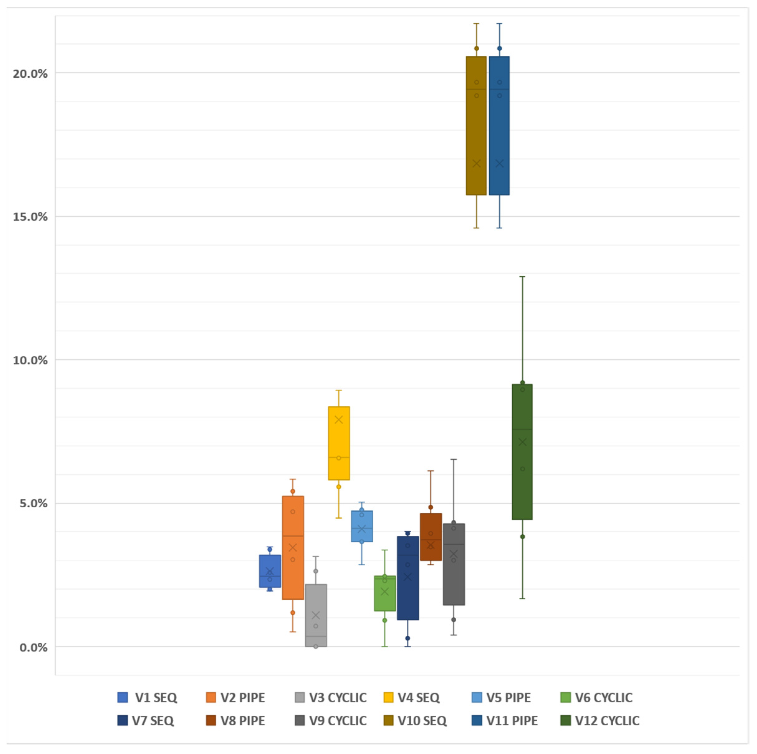
• Different neighborhood structures are extensively tested on the benchmark instances, and the performance of the structures in terms of algorithm speed and efficiency are shown.
• Several VNS variants are investigated, and the results are compared in detail.

In this paper, we address a particular variant of the EVRP, where goods are assumed to be transported from different origins to different destinations, and each customer has both delivery and pickup needs that must be met simultaneously. The structure of the paper is as follows: Section 2 reviews the scientific literature, while Section 3 proposes an integer linear programming model for EVRP-SPD. Section 4 describes the solution heuristics, neighborhood structures, and operators used to find the best solutions for benchmark instances. In Section 5, optimal solutions for small instances derived from the CPLEX solver are compared with the heuristic solution method in terms of solution quality and CPU time. In addition, some illustrative numerical examples are analyzed. Finally, in Section 6, the conclusions are presented, and some future work is described.

2. Literature Review

The Vehicle Routing Problem (VRP) was first introduced in the literature by Dantzig and Ramser [3]. The VRP is an important combinatorial optimization problem in transportation and logistics. The classical VRP is defined as finding routes that serve a given number of customers, where the routes start and end at a central depot, each customer is served exactly once, the total time is constrained, and the vehicle capacity is limited. The main objective is generally to minimize costs. The VRP has been expanded to include several variants as different constraints have been added from real-world uses.

Interest in the Electric Vehicle Routing Problem (EVRP) has been increasing in recent years, as the use of EVs in logistics operations has increased. EVRP is an NP-hard problem in which routing and charging plans are optimized simultaneously [4]. Charging strategy assumptions can be classified as partial and fully charging. Charging the battery fully takes longer, so it affects the solution in terms of time. Partial charging of the battery is more practical because it takes less time. The battery only needs to be charged enough to visit customers on the route and return to the depot, eliminating unnecessary charging time. In addition, charging EVs at the depot is cheaper than at charging stations, and the overall cost of charging can be reduced with partial charging [5,6]. Felipe, Ortuño, Righini, and Tirado [6]; Bruglieri et al. [7]; and Keskin and Catay [8] have considered partial charging strategies in which battery charging of EVs is adjusted at each charging station. Desaulniers et al. [9] proposed the EVRPTW and designed four variants with single or multiple charges per tour and partial or full charges.

Montoya et al. [10] developed a mixed-integer linear programming formulation with a nonlinear charging function and a hybrid metaheuristic to minimize the total time (driving and charging time). They tried to find an efficient charging plan under the fixed route assumption. Lin et al. [11] focused on the EVRP by taking into account the effect of payload on the battery consumption rate. They assumed charging time of EVs is constant, and EV load capacity was not considered. Erdoĝan and Miller-Hooks [12] developed a modified Clarke and Wright Savings heuristic to solve the Green Vehicle Routing Problem. Some assumptions included constant charging time and linear energy consumption with distance traveled. On the contrary, Kancharla and Ramadurai [13] assumed nonlinear charging time and load-dependent energy consumption. Strehler et al. [14] proposed a solution approach for a mixed fleet in which electric and hybrid vehicles are routed based on different strategies. In this context, they developed a mathematical model for both types of vehicles that tries to find the shortest path, use recyclable sources, and find charging stations. In the literature, there are other studies that assume nonlinear charging times, such as Froger et al. [15], Keskin et al. [16], and Koç et al. [17].

In the real world, when deciding on the size of the fleet and the characteristics of the EVs in the fleet, companies must consider customer demand, the characteristics and quantity of the loads to be transported, regional legal obligations, the physical characteristics of the demand points, and so on. In the literature, this problem is commonly referred to as the fleet size and mix (FSM) problem, and there are studies that focus on this problem in electric vehicle routing. Goeke and Schneider [18] studied the EVRPTW with a mixed fleet (E-VRPWTMF) of EVs and internal combustion engine vehicles. They investigated the effects of load and various objectives. They developed an accurate model for energy consumption. Hiermann et al. [19] considered time windows and charging stations to solve the electric fleet size and vehicle mix routing problem (E-FSMFTW). Hiermann et al. [20] presented a routing problem for a mixed fleet with different vehicle types, e.g., internal combustion engine vehicles, plug-in hybrids, and EVs.

In real-world applications, the time window is another essential constraint for EVRP. Schneider, Stenger, and Goeke [1] studied the EVRP with a time window (EVRPTW) for the first time in the literature. They assumed charging would be linear and EVs would be fully charged. Keskin, Laporte, and Catay [16] considered that charging stations have limited capacity. They also assumed time windows and time-dependent waiting times using a queuing system for charging stations. Lu et al. [21] considered the impact of traffic during peak hours for the time-dependent EVRP.

The location of charging stations has been combined with EVRP in some recent studies. Yang and Sun [22] presented the problem of battery-swap station locations for EVs with that capacity (BSS-EV-LRP). The authors developed models and four-phase and two-phase heuristic methods to solve the problem. Li-Ying and Yuan-Bin [23] presented the multiple EV charging station siting problem with time windows (EV-MCS-LRPTW) to optimize both infrastructure selection and charging station siting. Schiffer and Walther [5], Hof et al. [24], and Gatica et al. [25] proposed a novel EV location system that can simultaneously find charging stations and route EVs. Zhang et al. [26] constructed the routing problem for finding electric battery replacement stations with stochastic requirements. Paz et al. [27] proposed the electric location routing problem with time windows for multiple depots. The Electric Vehicles Integrated Planning Problem (EVs-IPP) was presented by Arias et al. [28]. The optimal placement of charging stations was performed considering the routes of EVs and the impact on the power-distribution system. Chen et al. [29] propose the problem of location and routing battery swap stations with time windows and a mixed fleet of electric and conventional vehicles (BSS-MF-LRPTW). Çalık et al. [30] assumed a heterogeneous fleet of EVs with limited capacity in solving the EVLRP.

One of the extensions of the EVRP is the pickup-and-delivery problem (PDP), where a customer must either be delivered or picked up. To the best of our knowledge, there are six journal articles in the current literature that propose different approaches to solving the electric vehicle routing problem with pickup and delivery and time windows (EVRP-PDP-TW). In this context, Lin, Zhou, and Wolfson [11] introduced the assumption that vehicle load affects battery consumption, and Zhao and Lu [31] considered a heterogeneous EV fleet with fixed charging times at charging stations. Grandinetti et al. [32] and Yang et al. [33] also proposed a homogeneous EV fleet with a linear charging function. Goeke [34] and Ahmadi et al. [35] both assume partial charging with linear and nonlinear charging functions, respectively. Ghobadi et al. [36] propose a multi-depot pickup and delivery problem for EVs with fuzzy time windows. Soysal et al. [37] studied the impact of stochastic battery discharge of EVs by visiting battery swap stations instead of charging stations for EVRP-PDP. Nolz et al. [38] developed an ALNS-based procedure to solve EVRP-PDP under the assumptions of a linear charging function, partial charging, and a heterogeneous EV fleet.

In summary, the current EVRP literature is limited to studies in which customer demand implies either delivery only or non-simultaneous delivery and pickup. To our knowledge, there is no study of EVRP in the literature that considers simultaneous pickup and delivery.

Table 1. EVRP with pickup and delivery in the literature.

Paper	SPD	PDP	TW	PD	BSS	MD	DM	ECM	OCM	TM	HEF	PC	CF
Grandinetti, Guerriero, Pezzella, and Pisacane [32]		✓	✓				✓		✓				L
Lin, Zhou, and Wolfson [11]		✓					✓	✓			✓		L
Goeke [34]		✓	✓				✓					✓	L
Zhao, and Lu [31]		✓	✓					✓	✓		✓		FT
Soysal, Cimen, and Belbag [37]		✓			✓			✓
Ahmadi, Tack, Harabor, and Kilby [35]		✓	✓							✓		✓	NL
Ghobadi, Tavakkoli Moghadam, Fallah, and Kazemipoor [36]		✓	✓			✓			✓				FT
Yang, Ning, Tong, and Shang [33]		✓	✓					✓	✓			✓	L
Nolz, Absi, Feillet, and Seragiotto [38]		✓							✓			✓	L

SPD: Simultaneous Pickup and Delivery; PDP: Pickup and Delivery Problem; TW: Time Windows; PD: Partial Delivery; BSS: Battery Swap Station; MD: Multi-Depot; DM: Distance Minimization; ECM: Energy Cost Minimization; OCM: Other Costs Minimization; TM: Time Minimization; HEF: Heterogenous Fleet; PC: Partial Charging; L: Linear Charging Function; FT: Fixed Time; NL: Non-linear Charging Function.

provides a summary of the literature on EVRP with pickup and delivery.

3. Mathematical Model

In this work, we address the problem of designing a network that simultaneously delivers/picks up freight from a central depot to customers and vice versa using EVs that need to visit multiple charging stations due to their limited range. In this context, the assumptions of EVRP-SPD can be formulated as follows: A group of customers is located in a distribution network in which customers require both deliveries and pickups. Partial deliveries and partial pickups are not allowed. Each customer must be served once for both operations with a given fleet of identical EVs; the EV fleet is homogeneous. Each vehicle leaves the central depot with the total amount of goods to be delivered and returns to the depot with the total amount of goods picked up. The vehicle load cannot exceed the vehicle capacity at any time during the tour. The capacity of the depot is unlimited. An EV visiting the charging station leaves with a full load; partial loads are not allowed. Charging stations may be visited more than once by the same EV. It is assumed that EVs are charged at a constant rate at charging stations. The objective function is to minimize the total distance traveled by the EVs.

An integer-model program based on three index nodes with the following notation is proposed for EVRP-SPD:

Notation and Sets

$n_d=\mathrm{number} \mathrm{of} \mathrm{depots}$

$n_r=\mathrm{number} \mathrm{of} \mathrm{charging} \mathrm{stations}$

$n_c=\mathrm{number} \mathrm{of} \mathrm{customers}$

$n_k=\mathrm{number} \mathrm{of} \mathrm{EVs}$

$N_D=\mathrm{the} \mathrm{set} \mathrm{of} \mathrm{depot} \left\{1, \dots , n_d\right\}$

$N_R=\mathrm{the} \mathrm{set} \mathrm{of} \mathrm{charging} \mathrm{stations} \left\{n_d+1, \dots , n_d+n_r\right\}$

$N_C=\mathrm{the} \mathrm{set} \mathrm{of} \mathrm{customers} \left\{n_d+n_r+1, \dots , n_d+n_r+n_c\right\}$

$N_{RC}=\mathrm{the} \mathrm{set} \mathrm{of} \mathrm{charging} \mathrm{stations} \mathrm{and} \mathrm{customers} \left\{n_d+1, \dots ,n_d+n_r+n_c\right\}$

$N_{DRC}=\mathrm{the} \mathrm{set} \mathrm{of} \mathrm{depots}, \mathrm{charging} \mathrm{stations} \mathrm{and} \mathrm{customers} \left\{n_d, \dots , n_d+n_r+n_c\right\}$

$N=\mathrm{the} \mathrm{set} \mathrm{of} \mathrm{nodes} \left\{1, \dots , n_d+n_r+n_c\right\}$

$N_k=\mathrm{the} \mathrm{set} \mathrm{of} \mathrm{EVs} \mathrm{at} \mathrm{the} \mathrm{depot} \left\{1, \dots , n_k\right\}$

Parameters

$d_{ij}= \mathrm{distance} \mathrm{from} \mathrm{nodes} i \mathrm{to} j$

$Q_k=\mathrm{maximum} \mathrm{loading} \mathrm{capacity} \mathrm{of} \mathrm{EV} k$

$B{C}_k=\mathrm{maximum} \mathrm{battery} \mathrm{capacity} \mathrm{of} \mathrm{EV} k$

$g_k=\mathrm{charging} \mathrm{rate} \mathrm{of} \mathrm{EV} k$

$h_k=\mathrm{energy} \mathrm{consumption} \mathrm{rate} \mathrm{of} \mathrm{EV} k$

$D_j=\mathrm{delivery} \mathrm{goods} \mathrm{demand} \mathrm{of} \mathrm{customer} j \left(\forall j\in N_C\right)$

$P_j= \mathrm{pick}-\mathrm{up} \mathrm{goods} \mathrm{demand} \mathrm{of} \mathrm{customer} j\left(\forall j\in N_C\right)$

Decision Variables

$x_{kij}=\left\{\begin{array}{ll}1,& if node j visited by EV k \mathit{after} \mathit{node} i;\\ 0,& otherwise\end{array}\right.\hspace{1em}\left(\forall k \in N_k , \forall i,j\in N_D\cup N_R\cup N_c\right)$

$U_{kij}=\mathrm{amount} \mathrm{of} \mathrm{goods} \mathrm{to} \mathrm{be} \mathrm{delivered} \mathrm{by} \mathrm{EV} k \mathrm{on} \mathrm{the} \mathrm{arc} (i,j) \left(\forall i,j\in N, \forall k\in N_k\right)$

$V_{kij}=\mathrm{amount} \mathrm{of} \mathrm{goods} \mathrm{picked}-\mathrm{up} \mathrm{by} \mathrm{EV} k \mathrm{on} \mathrm{the} \mathrm{arc} (i,j) \left(\forall i,j\in N, \forall k\in N_k\right)$

$BSC{a}_{ik}=\mathrm{charge} \mathrm{level} \mathrm{of} \mathrm{EV} k \mathrm{upon} \mathrm{arrival} \mathrm{at} \mathrm{node} i \left(\forall i\in N, \forall k\in N_k\right)$

$BSC{d}_{ik}= \mathrm{charge} \mathrm{level} \mathrm{of} \mathrm{EV} k \mathrm{at} \mathrm{departure} \mathrm{from} \mathrm{node} i \left(\forall i\in N, \forall k\in N_k\right)$

MODEL

$$Min Z={\displaystyle \sum }_{k\in N_k}{\displaystyle \sum }_{i\in N}{\displaystyle \sum }_{j\in N}{d}_{ij}\ast x_{kij}$$

(1)

$${{\displaystyle \sum }}_{k\in N_k}{{\displaystyle \sum }}_{i\in N}{x}_{kij}=1, \forall j\in N_C$$

(2)

$${{\displaystyle \sum }}_{i\in N}{x}_{kji}-{{\displaystyle \sum }}_{i\in N}{x}_{kij}=0, \forall k\in N_k , \forall j\in N$$

(3)

$${{\displaystyle \sum }}_{j\in N_{RC}^{\prime }}{x}_{kij}\le 1, \forall k\in N_k , \forall i\in N_D$$

(4)

$${{\displaystyle \sum }}_{j\in N_{RC}^{\prime }}{x}_{kji}\le 1, \forall k\in N_k , \forall i\in N_D$$

(5)

$$U_{kij}=0, \forall i\in N_{RC} , \forall j\in N_D,\forall k\in N_k$$

(6)

$$V_{kji}=0, \forall i\in N_{RC} , \forall j\in N_D,\forall k\in N_k$$

(7)

$$U_{kij}+V_{kij}\le Q_k\ast x_{kij}, \forall i,j\in N, \forall k\in N_k$$

(8)

$$x_{kii}=0, \forall i\in N, \forall k\in N_k$$

(9)

$$BSC{a}_{ik}\ge 0, \forall i\in N, \forall k\in N_k$$

(10)

$$BSC{d}_{ik}=B{C}_k, \forall i\in N_D, \forall k\in N_k$$

(11)

$$BSC{a}_{jk}\le BSC{a}_{ik}-\left(h_k\ast d_{ij}\right)\ast x_{kij}+B{C}_k\ast \left(1-x_{kij}\right), \forall i\in N_C ,\forall j\in N, i\ne j,\forall k\in N_k$$

(12)

$$BSC{a}_{jk}\le BSC{d}_{ik}-\left(h_k\ast d_{ij}\right)\ast x_{kij}+B{C}_k\ast \left(1-x_{kij}\right), \forall i,j\in N, i\ne j, \forall k\in N_k$$

(13)

$$BSC{a}_{ik}\le BSC{d}_{ik}, \forall i\in N, \forall k\in N_k$$

(14)

$$BSC{d}_{ik}\le B{C}_k, \forall i\in N, \forall k\in N_k$$

(15)

$$BSC{a}_{ik}=BSC{d}_{ik}, \forall i\in N_C, \forall k\in N_k$$

(16)

$$BSC{d}_{ik}=B{C}_k, \forall i\in N_R, \forall k\in N_k$$

(17)

$${{\displaystyle \sum }}_{i\in N}{U}_{kij}={{\displaystyle \sum }}_{i\in N}{U}_{kji}, \forall j\in N_R, \forall k\in N_k$$

(18)

$${{\displaystyle \sum }}_{i\in N}{V}_{kij}={{\displaystyle \sum }}_{i\in N}{V}_{kji}, \forall j\in N_R, \forall k\in N_k$$

(19)

$${{\displaystyle \sum }}_{k\in N_k}{{\displaystyle \sum }}_{i\in N}{U}_{kij}-{{\displaystyle \sum }}_{k\in N_k}{{\displaystyle \sum }}_{i\in N}{U}_{kji}=D_j, \forall j\in N_{RC}$$

(20)

$${{\displaystyle \sum }}_{k\in N_k}{{\displaystyle \sum }}_{i\in N_{DRC}^{\prime }}{V}_{kij}-{{\displaystyle \sum }}_{k\in N_k}{{\displaystyle \sum }}_{i\in N_{DRC}^{\prime }}{V}_{kji}=P_j, \forall j\in N_{RC}$$

(21)

$$d_{ij}\ge x_{kji}, \forall i,j\in N, \forall k\in N_k$$

(22)

$$x_{kij}\in \left\{0,1\right\}, \forall \mathrm{k}\in N_k, \forall \mathrm{i},j\in N_D\cup N_R\cup N_C$$

(23)

$$U_{kij}, BSC{a}_{ik}, BSC{d}_{ik},V_{kij}\ge 0, \forall \mathrm{i},j\in N, \forall \mathrm{k}\in N_k$$

(24)

The objective function (1) aims to minimize the total distance traveled by EVs. Constraint (2) ensures that each customer is visited exactly once, while Constraint (3) ensures that EVs depart immediately after visiting a customer or charging station, and that EVs leaving the depot return to the depot. Constraints (4), (5), and (22) allow EVs to be used only when needed at the depot. Constraint (6) states that no goods are delivered in EVs returning to the depot from the customer. Constraint (7) states that no goods will be picked up in EVs traveling from the depot to the customer. Constraint (8) states that the total number of goods picked up and to be delivered by the EV shall not exceed the capacity of the EV. Constraint (9) prevents the formation of a sub-tour with an element by preventing a trip from the current node to the node itself. Constraint (10) ensures that the charge level of EV $k$ upon arrival at node $i$ shall not be negative. Constraint (11) states that EVs leave the depot fully charged. Constraint (12) ensures that the charge level of vehicle $k$ arriving at node $j$ is less than or equal to the charge level arriving at node $i$. Constraint (13) ensures that the charge level of vehicle $k$ arriving at node $j$ is less than or equal to the charge level at departure from node $i$. Constraints (14)–(17) are other constraints related to the battery state of charge. Constraint (18) states that the amount of goods to be delivered by an EV visiting the charging station remains the same, while Constraint (19) states that the amount of goods picked up remains the same. Constraints (20) and (21) ensure that customer demand for the goods to be delivered and the goods to be picked up are satisfied by the same EV. Constraints (23) and (24) define the nature of the variables.

4. The Proposed Solution Methodology

Considering the complexity of the problem, we developed a metaheuristic solution approach based on the VNS algorithms to solve the EVRP-SPD. Several variants of the VNS solution approach were implemented in this methodology. A modified Clark and Wright Savings algorithm, which takes into account the assumptions and characteristics of the problem, was developed to obtain a feasible initial solution. Algorithm 1 details the creation of a feasible initial solution. In addition to the shaking and local search operators of the VNS, we also used well-known destruction and repair operators to improve the performance of the VNS. VNS was first proposed by Mladenović and Hansen [39]. The basic idea is to explore distant neighborhoods of the current solution and switch to a new solution only when improvement has been achieved. It is widely used to solve different variants of VRPs [1,7,29,40,41,42,43,44,45]. In this paper, we integrated the features of the proposed problem into the VNS. The details of the proposed solution approach are described in Algorithm 2.

Algorithm 1 Modified CW Savings Algorithm for EVRP-SPD

1: Start 2: while There are customers not added to the routes do 3:      Create back-forth (BF) tours (depot-customer-depot) 4:      if EV charge level insufficient to complete the tour then 5:      Add the CS with the lowest cost to the tour 6:      if energy constraint is not met then 7:        Cancel the tour and remove from tour list 8:        Add customer to the list of unvisited customers 9:      else 10:       Add the tour to the tour list 11:     end if 12:     else 13:     Add the BF tour to the tour list 14:     end if 15: end while 16: Create savings list by computing the savings 17: Sort the savings in descending order 18: while the savings list is not empty do 19:     Select two BF tours with largest savings 20:     if customer(s) have already been added to the current tours then 21:     Cancel the merge 22:     Remove the relevant customer pair from the savings list 23:     else 24:     Check remaining capacity of EV 25:     if capacity constraint is not met then 26:         Cancel the merge 27:         Remove the relevant customer pair from the savings list 28:     else 29:       Check remaining charge level of EV 30:       if energy constraint is not met then 31:        Add CS to the tour with minimum cost 32:        if energy constraint is not met then 33:         Cancel the merge 34:         Remove the relevant customer pair from the savings list 35:        else 36:         Merge selected BF tours 37:         Update the tour list 38:        end if 39:       else 40:        Merge selected BF tours 41:        Update the tour list 42:       end if 43:     end if 44:     end if 45:     Update the savings list based on new tour list 46: end while 47: Add customers from the list of unvisited customers to existing tours using the greedy insertion operator 48: End

Algorithm 2 VNS Framework

1: Function VNS Variants ($x, k_{max}, N$) 2: $f_{best}\leftarrow x$ Initial Solution 3: while the stopping condition is not fulfilled do 4:  $k\leftarrow 1$ 5:  while $k\le k_{max}$ do 6:  $x^{\prime }\leftarrow$ Shake ($x, k, N$); 7:  $x^{″}\leftarrow$ Local Search ($x^{\prime },N$); 8:  Neighborhood Change: Sequential or Pipe or Cyclic ($x,x^{″},k$); 9:  if $f_{\left(x^{″}\right)}<f_{best}$ then 10:    $x\leftarrow x^{″}$; $f_{best}=f_{\left(x\right)}$; 11:   end if 12:  end while 13: end while 14: Return $x$

4.1. Construction of the Initial Solution

To generate a feasible initial solution, we employ the savings heuristic proposed by Clarke and Wright [46] for EVRP-SPD. There are variations of saving heuristics developed for VRP and its extensions in the literature, but to our knowledge, a version for EVRP-SPD does not yet exist. To this end, we have adapted a savings heuristic that takes into account the limited range of EVs and simultaneous pickup and delivery.

Unlike the original method, a greedy insertion operator inserts a charging station with the maximum savings value (minimum insertion cost) into the back–forth tour (depot–customer–depot). If the battery constraint is not met even after the charging station is added, the relevant tour is removed, and the customer in the tour is added to the list of unvisited customers ($L_{unvisited})$. A savings list is generated that includes each pair of customers in back-and-forth tours and the savings values of those pairs. To calculate the savings values of each pair of customers, we used the formulation proposed by Clarke and Wright [46]. In Equation (25), $d_{i0}$, $d_{0j}$, and $d_{ij}$ represent the distances between the depot and customer $i$, the depot and customer $j$, and customer $i$ and customer $j$, respectively.

$$s_{ij}=d_{i0}+d_{0j}-d_{ij}$$

(25)

After the saving list is created, the list is sorted in descending order of savings values. Then, tours involving those customers are merged, starting with the pair of customers with the greatest savings value. If the new tour violates vehicle capacity, the merge is canceled, the relevant customer pair is removed from the savings list, and the merge continues with the next customer pair with the highest savings value. If the new tour violates battery constraint, the charging station with the minimum insertion cost is added to the tour. Minimum insertion cost represents the one that increases the tour distance the least among all possible charging stations, which, when added to the tour, makes the tour convenient. If feasibility cannot be achieved even after the charging station is added, a second charging station is not added, and the merge process is canceled. The relevant customer pair is removed from the savings list. The cycle continues with the next customer pair with the highest savings value until there are no pairs of customers left on the savings list. After merging of the tours is complete, the customers that have not yet been visited ($L_{unvisited})$ are inserted into the created tours using a greedy insertion operator.

4.2. Variable Neighborhood Search

Metaheuristics are expected to explore the solution space efficiently to find good-quality solutions and to do so as quickly as possible. By using multiple neighborhood structures and changing them systematically during the search, VNS has an excellent ability to explore the search space and shows superior performance over its competitors [1,7,21,24,43,47,48,49]. While shaking operators are used to diversify the search and to explore different neighborhoods, local search operators are used to find the local optima of a particular neighborhood. Therefore, it is crucial to choose the best neighborhood operators to obtain high-quality solutions to the problem.

In this work, different VNS variants, such as reduced VNS (RVNS), basic VNS (BVNS), general VNS (GVNS), nested VNS (NVNS), and random VNS (RNDVNS), and different neighborhood change steps, such as sequential, pipe, and cyclic, were tested to solve the EVRP-SPD. The purpose of the neighborhood change steps is to guide the VNS in exploring the solution space. In other words, it decides which neighborhood to explore after the incumbent solution and which solution or solutions to accept as the new incumbent solution(s). Commonly used neighborhood change steps are sequential, pipe, and cyclic [50]. In sequential neighborhood change, exploration continues in the first neighborhood structure of the new incumbent solution if improvement in the incumbent solution occurs in any neighborhood structure; otherwise, exploration continues in the next neighborhood. Regardless of whether there is improvement in the incumbent solution in the current neighborhood, exploration continues in the next neighborhood structure in the cyclic neighborhood change step, whereas in the pipe neighborhood change step, exploration continues in the current neighborhood. In this work, sequential, pipe, and cyclic neighborhood change steps are used in the VNS variants. Details can be found in

Table 2. Neighborhood change steps considered in VNS variants.

NCS	BVNS	GVNS	RVNS	RNDVNS	NVNS
Sequential	(v4)	-	(v1)	(v7)	(v10)
Pipe	-	(v5)	(v2)	(v8)	(v11)
Cyclic	-	(v6)	(v3)	(v9)	(v12)

.

Reduced VNS is a variant of the VNS heuristic introduced by Mladenović and Hansen [39] for solving combinatorial optimization problems [51,52,53]. RVNS is practical for large instances where local search is computationally intensive. Instead of searching for all solutions of a neighborhood structure, RVNS randomly selects one solution and immediately performs the neighborhood change step. Another variant of VNS is basic VNS, which examines neighborhood structures in a predefined order. If the solution improves when any neighborhood structure is applied, the search should be restarted at the first structure [54]. Therefore, BVNS uses a sequential step to change the neighborhood. General VNS uses local search with variable neighborhood descent (VND) within the BVNS scheme [55]. A simplification of VNS, called nested VNS, consists of applying a VNS variant to each point of a predefined nested (combined) neighborhood structure as a local search procedure [56]. Random VNS (RNDVNS) differs from BVNS by selecting the nearest neighborhood structure to visit. RNDVNS consists of randomly selecting an unvisited neighborhood to continue the search when a neighborhood structure cannot find an improved solution [57]. This variant does not depend on a predetermined order of visits to neighborhood structures.

For a pseudocode overview of the VNS and its variants, see Algorithm 2. First, the algorithm takes as input an initial solution generated by the modified C&W savings algorithm. A local search phase is used to improve the solution, and a shaking phase is used to avoid local minima traps. The neighborhood change step is performed sequentially until a predefined stop condition is satisfied. In this study, a reasonable time limit considering the problem size of datasets is applied as a termination criterion on the same hardware configuration. Thus, a fair performance comparison among algorithms is provided.

4.3. Neighborhood Structures

The neighborhood structures used in this work are described below. They are based on neighborhoods used in the VRP and EVRP literature. Four inter-route operators (replace, cross, exchange, and shift) and five intra-route operators (swap, 2-opt, 3-opt, insert customer, and insert charging station) are used, while six removal operators (Shaw customer, maximum distant n customer, random n customer, minimum capacity route, random route, and maximum distant one customer removal) are used in the shaking step. When a removal operator is used in the shaking step, repair operators (inserting a distance base, inserting a greedy customer, and creating a route from the list of removed customers) are used in the local search step. Further, four operators for best move (best swap of customers, best swap of all customers and charging stations), best insertion, and best reverse route) are used in the local search step. See

Table 3. VNS neighborhood structures.

Name	Applied to		Name	Applied to
Shaking Step	C	CS	Local Search Step	C	CS
Swap	✓		Best Swap Customer	✓
2-Opt	✓		Best Swap All	✓	✓
3-Opt	✓	✓	Best Insert	✓
Insert Customer (C)	✓		Best Reverse Route	✓	✓
Insert Charging Station (CS)		✓
Replace	✓
Cross	✓
Exchange	✓
Shift	✓
Shaking Step	Description			C	CS
Shaw Customer Removal	SeedC (Random), C (Similarity)			✓
Maximum Distant N Customer Removal	N (Random), C (Distance)			✓
N Random Customer Removal	N (Random), C (Random)			✓
Minimum Capacity Route Removal	R (Min Cap)			✓	✓
Random Route Removal	R (Random)			✓	✓
Maximum Distant One Customer Removal	C (Distance)			✓
Local Search Step				C	CS
Distance Base Insertion	Distance Change (Calc by Whole Route)			✓
Greedy Customer Insert	Distance Change (Calc by Pred. and Succ. Nodes)			✓
Create a Route from List of Removed	Creates Routes from Single Customers that Cannot be Added to the Same Route			✓

C: Customer, CS: Charging Station.

for details on the neighborhood structures.

5. Numerical Investigations

5.1. Implementation

Experiments with the proposed solution approaches and CPLEX were performed on a machine with an Intel Core i7-9750H CPU with 6 cores at 2.60 GHz and at least 16GB RAM. The mathematical model we developed for EVRP-SPD was solved using CPLEX 12.1 in one-threaded mode for small instances. The proposed algorithms were coded in MATLAB, a simple and effective programming language. Moreover, each experiment was performed in one-threaded mode using the asynchronous structure of the Parallel Computing Toolbox of MATLAB R2020b. Thus, by taking advantage of this parallel computing structure, replications of the experiments were obtained sooner than if the experiments had been run in sequence. CPLEX, on the other hand, was used to obtain exact results for small instances and to confirm that the VNS algorithms can reach these optimal results.

5.2. Generation of EVRP-SPD Instances

There is no available instance set for EVRP-SPD, as the problem has not yet been studied in the literature. Therefore, we created new instance sets to test our solution approach. EVRP-SPD instances were derived from EVRP-TW instance sets by Schneider, Stenger, and Goeke [1]. The original instance sets have 36 small and 56 large instances, but in this study 36 small and 34 large instances were derived from the instance sets by Schneider, Stenger, and Goeke [1] for EVRP-SPD. While all large instances from Schneider, Stenger, and Goeke [1] are identical in terms of customer and charging station locations, the 34 large instances differed in terms of pickup and delivery requirements, battery, and load capacity of EVs in EVRP-SPD. The small instances consisted of 5, 10, and 15 customers, and the large instances included 100 customers and 21 charging stations. There were three types of instances in terms of geographical distribution of customer coordinates: random distribution (R), clustered distribution (C), and a combination of both (RC).

One of the precautions taken in the datasets used was to redetermine customer demand in accordance with the model. The simultaneous pickup and delivery constraint requires two different sets of demand data for each customer, for both pickup and delivery. In this context, customer demand was recalculated in the original dataset, as in the method used by Salhi and Nagy [2].

In this method, a coefficient $k_i=\min \left(x_i/y_i,y_i/x_i\right)$ is determined based on the coordinates of each customer $\left(x_i,y_i\right)$. Then, this coefficient and customer demand $\left(q_i\right)$ of the original dataset are used to calculate the delivery $\left(D_i\right)$ and pickup $\left(P_i\right)$ demand of each customer. The equations $D_i=k_i\ast q_i$ and $P_i=k_i\ast q_i$ are used for delivery and pickup demand, respectively.

5.3. Neighborhood Structure Tests on Instances

In this section, 26 neighborhood structures were tested on three types of instances with respect to the geographic distribution of customer coordinates (C, R, and RC) to decide which neighborhoods to use and in what order. All operators of the shaking and local search steps started with the same solution ($x$) in their own step, since it is important that each operator competes under the same conditions. New neighborhoods $(N_s, s=1,\dots , s_{max})$ explored by each operator in the shaking step are determined as the incumbent solutions ($x^{\prime }$) for each local search operator. Then, new neighborhoods $(N_l, l=1,\dots , l_{max})$ are explored by each operator in the local search. Similarly, the fitness values of the newly explored neighborhoods are compared, and the best one is determined as the incumbent solution ($x^{″}$), so that one iteration is completed. This cycle continues until the established termination criteria are met. In summary, the average success rate ($AS{R}_k$) of each operator can be calculated as follows:

$$AS{R}_k=100\ast \left(N{S}_k/N{T}_k\right)$$

(26)

where $N{S}_k$ represents the number of successes of the $k$’th operator. Success means that a new neighborhood with better fitness is explored. $N{T}_k$ represents the total number of attempts of the $k$’th operator. The average success rates of the most successful operators used in this work are shown in descending order for small and large instances in Figure 2 and Figure 3, respectively.

Algorithm 3 Neighborhood Structure (NS) Performance Test Algorithm

1: Function Fair Performance Comparison 2: Select the set of NS for Shake Phase ($S{H}_i, i=1, \dots , i_{max}$) 3: Select the set of NS for Local Search Phase ($L{S}_j, j=1, \dots , j_{max}$) 4: $No{S}_{S{H}_i}\leftarrow 0$ // Initialize No of Success for $S{H}_i$ 5: $No{S}_{L{S}_j}\leftarrow 0$ // Initialize No of Success for $L{S}_j$ 6: $No{T}_{S{H}_i}\leftarrow 0$ // Initialize No of Total Usage for $S{H}_i$ 7: $No{T}_{L{S}_j}\leftarrow 0$ // Initialize No of Total Usage for $L{S}_j$ 8: $AS{R}_{S{H}_i}$: Average Success Rate of $S{H}_i$ 9: $AS{R}_{L{S}_j}$: Average Success Rate of $L{S}_j$ 10: $x_{best}\leftarrow$ Initial Solution by Modified CW Savings 11: while the stopping condition is not fulfilled do 12:  $x\leftarrow x_{best}$; 13:  for $i=1:i_{max}$ do 14:    $x_i^{\prime }\leftarrow$ Shake ($x,S{H}_i$); 15:    $No{T}_{S{H}_i}=No{T}_{S{H}_i}+1$; 16:    if $f_{\left(x_i^{\prime }\right)}<f_{\left(x\right)}$then 17:      $No{S}_{S{H}_i}=No{S}_{S{H}_i}+1$; 18:    end if 19:    if $f_{\left(x_i^{\prime }\right)}<f_{best}$then 20:      $x_{best}=x_i^{\prime }$; 21:    end if 22:    for $j=1:j_{max}$ do 23:      $x_j^{″}\leftarrow$ Local Search ($x_i^{\prime },L{S}_j$); 24:      $No{T}_{L{S}_j}=No{T}_{L{S}_j}+1$; 25:      if $f_{\left(x_j^{″}\right)}<f_{\left(x_i^{\prime }\right)}$ then 26:        $No{S}_{L{S}_j}=No{S}_{L{S}_j}+1$; 27:      end if 28:      if$f_{\left(x_j^{″}\right)}<f_{best}$ then 29:        $x_{best}=x_j^{″}$; 30:      end if 31:    end for 32:  end for 33: end while 34: for $i=1:i_{max}$ do 35:  $AS{R}_{S{H}_i}=100\times No{S}_{S{H}_i}÷No{T}_{S{H}_i}$; 36: end for 37: for $j=1:j_{max}$ do 38:  $AS{R}_{L{S}_j}=100\times No{S}_{L{S}_j}÷No{T}_{L{S}_j}$; 39: end for 40: Return $x_{best}, AS{R}_{S{H}_i}, AS{R}_{L{S}_j}$

When operators were ranked by success rate, similar results were obtained for three different customer location groups (C, R, and RC), but different results were obtained in terms of problem size. For this reason, the same set of operators was used for the three types of instances. Since the success rates of the operators were different for large and small problems, two sets of operators were created in which the operators and their order were different. The operators that could not improve the solution, i.e., with a success rate of zero ($AS{R}_k=0\%$), were eliminated. Moreover, each neighborhood structure was ordered in descending order of success rate to reduce the solution time. The operator sets to solve all the problems in the corresponding instances are listed in

Table 4. Operator sets employed in small-sized and large-sized instances.

Small-Sized Instances	Large-Sized Instances
Shake	Shake
Replace	Replace
Exchange	Shift
Cross	Exchange
Shift	Cross
InsertCS	InsertCS
Swap	MinCapRouteRem
NRandCustRem	RandRouteRem
2-Opt	NRandCustRem
MaxDistant1CustRem	MaxDistantNCustRem
ShawCustRem	ShawCustRem
MaxDistantNCustRem	MaxDistant1CustRem
RandRouteRem	Swap
MinCapRouteRem	SingleCustRRem
3-Opt	InsertC
InsertC
Local Search	Local Search
BestSwapALL	BestInsert
BestInsert	BestSwapALL
BestSwapC	BestSwapC
BestRoutebyCS	BestRoutebyCS
DistBasedCustIns	DistBasedCustIns
GreedyInsert	GreedyInsert
LremTo1Route	LremTo1Route

.

5.4. Numerical Results

Small test instances for EVRP-SPD were used to analyze the performance of our VNS-based solution approaches. For this purpose, the instances were solved with VNS variants, and the results were compared with the optimal solution found by the commercial solver CPLEX 12.1 using the EVRP-SPD formulation presented in Section 3.

An overview of the results is given in

Table 5. Comparison of CPLEX vs. VNS variant results on small-sized instances.

				Reduced VNS									Basic VNS			General VNS
	CPLEX			V1 Seq			V2 Pipe			V3 Cyclic			V4 Seq			V5 Pipe			V6 Cyclic
Instance	$\mathit{f}$	$\mathit{t}$	${\Delta }_{\mathit{f}}$	$\mathit{f}$	$\mathit{t}$	${\Delta }_{\mathit{f}}$	$\mathit{f}$	$\mathit{t}$	${\Delta }_{\mathit{f}}$	$\mathit{f}$	$\mathit{t}$	${\Delta }_{\mathit{f}}$	$\mathit{f}$	$\mathit{t}$	${\Delta }_{\mathit{f}}$	$\mathit{f}$	$\mathit{t}$	${\Delta }_{\mathit{f}}$	$\mathit{f}$	$\mathit{t}$	${\Delta }_{\mathit{f}}$
C101C5	208.9	1.35	0%	208.9	0.05	0.00%	208.9	0.03	0.00%	208.9	0.05	0.00%	208.9	0.16	0.00%	208.9	0.16	0.00%	208.9	0.13	0.00%
C103C5	154.5	1.2	0%	154.5	0.17	0.00%	154.5	0.17	0.00%	154.5	0.2	0.00%	154.5	0.7	0.00%	154.5	0.34	0.00%	154.5	0.36	0.00%
C206C5	201.55	1.92	0%	201.55	0.03	0.00%	201.55	0.03	0.00%	201.55	0.03	0.00%	201.55	0.08	0.00%	201.55	0.06	0.00%	201.55	0.08	0.00%
C208C5	158.48	1.34	0%	158.48	0.06	0.00%	158.48	0.08	0.00%	158.48	0.08	0.00%	158.48	0.06	0.00%	158.48	0.06	0.00%	158.48	0.09	0.00%
R104C5 *	136.69	1.75	0%	136.69	0	-	136.69	0	-	136.69	0	-	136.69	0	-	136.69	0	-	136.69	0	-
R105C5 *	139.48	1.23	0%	139.48	0	-	139.48	0	-	139.48	0	-	139.48	0	-	139.48	0	-	139.48	0	-
R202C5	128.78	1.29	0%	128.78	1.73	0.00%	128.78	0.23	0.00%	128.78	0.33	0.00%	128.78	0.75	0.00%	128.78	0.36	0.00%	128.78	0.33	0.00%
R203C5	179.06	1.37	0%	179.06	0.22	0.00%	179.06	0.2	0.00%	179.06	0.2	0.00%	179.06	16.36	0.00%	179.06	6.14	0.00%	179.06	6.14	0.00%
RC105C5	208.43	1.89	0%	208.43	0.13	0.00%	208.43	0.13	0.00%	208.43	0.23	0.00%	208.43	0.75	0.00%	208.43	0.41	0.00%	208.43	0.34	0.00%
RC108C5	211.53	1.36	0%	211.53	0.25	0.00%	211.53	0.23	0.00%	211.53	0.22	0.00%	211.53	0.83	0.00%	211.53	0.41	0.00%	211.53	0.39	0.00%
RC204C5	176.39	2.54	0%	176.39	3.17	0.00%	179.16	1.36	1.60%	176.39	0.2	0.00%	179.16	1.13	1.60%	179.16	0.52	1.60%	179.16	0.52	1.60%
RC208C5	167.98	2.29	0%	167.98	0.02	0.00%	167.98	0.02	0.00%	167.98	0.02	0.00%	167.98	0.06	0.00%	167.98	0.05	0.00%	167.98	0.05	0.00%
C101C10	260.01	4.85	0%	260.01	5.67	0.00%	260.01	3.13	0.00%	260.01	7.36	0.00%	265.75	9.52	2.20%	260.01	13.96	0.00%	260.01	19.95	0.00%
C104C10	239.13	3.39	0%	239.13	4.98	0.00%	239.13	3.71	0.00%	239.13	1.53	0.00%	239.13	17.08	0.00%	239.13	9.12	0.00%	239.13	9.42	0.00%
C202C10	214.96	4.12	0%	214.96	7.2	0.00%	214.96	3.57	0.00%	214.96	8.73	0.00%	214.96	10.72	0.00%	214.96	6.03	0.00%	214.96	4.54	0.00%
C205C10	224.78	4.45	0%	227.08	0.79	1.00%	227.08	0.73	1.00%	224.78	0.36	0.00%	227.08	2.66	1.00%	227.08	1.73	1.00%	227.08	1.08	1.00%
R102C10	220.97	19.01	0%	220.97	0.74	0.00%	220.97	0.72	0.00%	220.97	2.44	0.00%	220.97	11.1	0.00%	220.97	2	0.00%	220.97	1.56	0.00%
R103C10	160.41	10.35	0%	160.41	3.87	0.00%	160.41	2.55	0.00%	160.41	11.17	0.00%	160.41	18.15	0.00%	160.41	16.38	0.00%	160.41	9.27	0.00%
R201C10	183.11	2.36	0%	197.54	1.9	7.90%	183.11	2.3	0.00%	183.11	4.73	0.00%	197.54	8.98	7.90%	183.11	15.55	0.00%	183.11	13.63	0.00%
R203C10	214.9	5.43	0%	214.9	2.3	0.00%	214.9	2.98	0.00%	214.9	2.88	0.00%	214.9	12.03	0.00%	214.9	6.27	0.00%	214.9	3.59	0.00%
RC102C10	346.7	4.03	0%	346.7	1.65	0.00%	346.7	5.57	0.00%	346.7	4.5	0.00%	354.31	6.55	2.20%	346.7	8.15	0.00%	346.7	7.12	0.00%
RC108C10	317.96	6	0%	317.96	13.13	0.00%	317.96	6.63	0.00%	317.96	3.3	0.00%	345.53	10.82	8.70%	317.96	20.73	0.00%	317.96	5	0.00%
RC201C10	246.99	5.26	0%	246.99	27.07	0.00%	246.99	26.49	0.00%	246.99	9.78	0.00%	247.26	16.97	0.10%	247.26	8.67	0.10%	247.26	11.8	0.10%
RC205C10	306.82	4.14	0%	306.82	0.79	0.00%	306.82	1.3	0.00%	306.82	0.92	0.00%	306.82	3.56	0.00%	306.82	1.94	0.00%	306.82	2.08	0.00%
C103C15	255.68	30.81	0%	255.68	49.81	0.00%	255.68	21.63	0.00%	255.68	34.23	0.00%	255.68	126.46	0.00%	255.68	20.29	0.00%	255.68	46.59	0.00%
C106C15	223.84	142.65	0%	223.84	172.21	0.00%	223.84	6.36	0.00%	223.84	88.61	0.00%	223.84	61.63	0.00%	223.84	16.1	0.00%	223.84	19.6	0.00%
C202C15	314.62	373.2	0%	326.57	205.19	3.80%	314.62	52.62	0.00%	314.62	129.31	0.00%	314.62	95.09	0.00%	314.62	48.33	0.00%	326.57	243.03	3.80%
C208C15	262.5	244.4	0%	262.5	7.55	0.00%	262.5	4.79	0.00%	262.5	2.84	0.00%	262.5	27.33	0.00%	262.5	6.05	0.00%	262.5	5.34	0.00%
R102C15	258.59	681.12	0%	258.59	110.03	0.00%	259.79	144.02	0.50%	258.59	23.27	0.00%	259.79	106.54	0.50%	258.59	49.21	0.00%	258.59	30.68	0.00%
R105C15	231.96	119.88	0%	231.96	40.64	0.00%	231.96	19.04	0.00%	231.96	11.73	0.00%	233.92	284.61	0.80%	231.96	29.16	0.00%	231.96	28.65	0.00%
R202C15	275.04	64.31	0%	275.04	42.01	0.00%	275.04	44.88	0.00%	275.04	13.64	0.00%	275.04	108.5	0.00%	275.04	36.39	0.00%	275.04	34.26	0.00%
R209C15	239.7	49.6	0%	239.7	10.76	0.00%	239.7	26.31	0.00%	239.7	9.22	0.00%	239.7	76.07	0.00%	239.7	239.62	0.00%	239.7	46.26	0.00%
RC103C15	291.07	52.73	0%	291.07	22.78	0.00%	291.07	22.25	0.00%	291.07	9.73	0.00%	291.07	62.43	0.00%	291.07	35.31	0.00%	291.07	34.67	0.00%
RC108C15	330.01	1197.23	0%	330.01	6.22	0.00%	330.01	5.76	0.00%	330.01	7.27	0.00%	330.01	61.84	0.00%	330.01	9.97	0.00%	330.01	26.47	0.00%
RC202C15	295.6	87	0%	319.32	85.21	8.00%	295.6	201.46	0.00%	295.6	94.69	0.00%	315.22	60.75	6.60%	295.6	50.44	0.00%	315.22	49.43	6.60%
RC204C15	255.68	30	0%	255.68	51.88	0.00%	255.68	16.12	0.00%	255.68	29.24	0.00%	255.68	118.24	0.00%	255.68	14.64	0.00%	255.68	40.24	0.00%
Avg.		87.94			24.45	0.60%		17.43	0.10%		14.25	0.00%		37.18	0.90%		18.74	0.10%		19.52	0.40%

* Optimal solution found by the C&W savings heuristic as the initial solution. Notes: $f$ denotes distance traveled; $t$ denotes CPU time in seconds; ${\mathsf{\Delta }}_f$ denotes the gap to the distance traveled found by CPLEX. Optimality is guaranteed for CPLEX results.

and

Table 6. Comparison of CPLEX vs. VNS variant results on small-sized instances.

				Random VNS									Nested VNS
	CPLEX			V7 Seq			V8 Pipe			V9 Cyclic			V10 Seq			V11 Pipe			V12 Cyclic
Instance	$\mathit{f}$	$\mathit{t}$	${\Delta }_{\mathit{f}}$	$\mathit{f}$	$\mathit{t}$	${\Delta }_{\mathit{f}}$	$\mathit{f}$	$\mathit{t}$	${\Delta }_{\mathit{f}}$	$\mathit{f}$	$\mathit{t}$	${\Delta }_{\mathit{f}}$	$\mathit{f}$	$\mathit{t}$	${\Delta }_{\mathit{f}}$	$\mathit{f}$	$\mathit{t}$	${\Delta }_{\mathit{f}}$	$\mathit{f}$	$\mathit{t}$	${\Delta }_{\mathit{f}}$
C101C5	208.90	1.35	0%	208.90	0.02	0.0%	208.90	0.02	0.0%	208.90	0.03	0.0%	208.90	0.16	0.0%	208.90	0.17	0.0%	208.90	0.16	0.0%
C103C5	154.50	1.20	0%	154.50	0.11	0.0%	154.50	0.17	0.0%	154.50	0.13	0.0%	154.50	0.33	0.0%	154.50	0.34	0.0%	154.50	0.28	0.0%
C206C5	201.55	1.92	0%	201.55	0.06	0.0%	201.55	0.08	0.0%	201.55	0.06	0.0%	201.55	0.02	0.0%	201.55	0.02	0.0%	201.55	0.02	0.0%
C208C5	158.48	1.34	0%	158.48	0.08	0.0%	158.48	0.06	0.0%	158.48	0.08	0.0%	158.48	0.05	0.0%	158.48	0.06	0.0%	158.48	0.09	0.0%
R104C5 *	136.69	1.75	0%	136.69	0.00	-	136.69	0.00	-	136.69	0.00	-	136.69	0.00	-	136.69	0.00	-	136.69	0.00	-
R105C5 *	139.48	1.23	0%	139.48	0.00	-	139.48	0.00	-	139.48	0.00	-	139.48	0.00	-	139.48	0.00	-	139.48	0.00	-
R202C5	128.78	1.29	0%	128.78	0.39	0.0%	128.78	0.38	0.0%	128.78	0.36	0.0%	128.78	0.39	0.0%	128.78	0.42	0.0%	128.78	0.38	0.0%
R203C5	179.06	1.37	0%	179.06	0.05	0.0%	179.06	0.03	0.0%	179.06	0.05	0.0%	179.06	2.39	0.0%	179.06	2.52	0.0%	179.06	1.80	0.0%
RC105C5	208.43	1.89	0%	208.43	0.16	0.0%	208.43	0.14	0.0%	208.43	0.14	0.0%	208.43	0.56	0.0%	208.43	0.52	0.0%	208.43	0.48	0.0%
RC108C5	211.53	1.36	0%	211.53	0.19	0.0%	211.53	0.19	0.0%	211.53	0.16	0.0%	211.53	0.63	0.0%	211.53	0.47	0.0%	211.53	0.44	0.0%
RC204C5	176.39	2.54	0%	179.16	0.59	1.6%	179.16	0.53	1.6%	179.16	0.55	1.6%	185.16	0.28	5.0%	185.16	0.27	5.0%	179.16	2.41	1.6%
RC208C5	167.98	2.29	0%	167.98	0.08	0.0%	167.98	0.06	0.0%	167.98	0.05	0.0%	167.98	0.05	0.0%	167.98	0.06	0.0%	167.98	0.23	0.0%
C101C10	260.01	4.85	0%	260.01	8.84	0.0%	260.01	3.51	0.0%	260.01	5.16	0.0%	260.01	11.94	0.0%	260.01	13.68	0.0%	260.01	29.00	0.0%
C104C10	239.13	3.39	0%	239.13	3.44	0.0%	239.13	2.95	0.0%	239.13	7.50	0.0%	239.13	19.18	0.0%	239.13	22.24	0.0%	239.13	20.90	0.0%
C202C10	214.96	4.12	0%	214.96	4.61	0.0%	214.96	4.61	0.0%	214.96	3.05	0.0%	231.07	8.79	7.5%	231.07	8.31	7.5%	214.96	7.32	0.0%
C205C10	224.78	4.45	0%	227.08	0.52	1.0%	224.78	3.52	0.0%	224.78	17.95	0.0%	227.08	1.76	1.0%	227.08	1.92	1.0%	227.08	1.32	1.0%
R102C10	220.97	19.01	0%	220.97	4.43	0.0%	220.97	3.54	0.0%	220.97	2.26	0.0%	220.97	7.22	0.0%	220.97	6.03	0.0%	220.97	4.36	0.0%
R103C10	160.41	10.35	0%	164.58	2.36	2.6%	160.41	23.15	0.0%	160.41	11.88	0.0%	164.58	7.59	2.6%	164.58	8.11	2.6%	160.41	15.17	0.0%
R201C10	183.11	2.36	0%	183.11	11.16	0.0%	183.11	11.25	0.0%	183.11	18.57	0.0%	197.54	2.92	7.9%	197.54	3.46	7.9%	183.42	26.99	0.2%
R203C10	214.90	5.43	0%	214.90	2.14	0.0%	214.90	2.34	0.0%	214.90	1.86	0.0%	214.90	2.58	0.0%	214.90	2.86	0.0%	214.90	2.32	0.0%
RC102C10	346.70	4.03	0%	346.70	6.80	0.0%	346.70	5.93	0.0%	346.70	5.64	0.0%	354.31	2.22	2.2%	354.31	1.83	2.2%	346.70	18.64	0.0%
RC108C10	317.96	6.00	0%	329.93	9.41	3.8%	317.96	8.42	0.0%	317.96	14.75	0.0%	317.96	23.79	0.0%	317.96	25.74	0.0%	317.96	26.44	0.0%
RC201C10	246.99	5.26	0%	247.26	12.70	0.1%	247.26	12.00	0.1%	247.26	11.98	0.1%	260.77	9.32	5.6%	260.77	11.06	5.6%	247.26	21.19	0.1%
RC205C10	306.82	4.14	0%	306.82	1.45	0.0%	306.82	1.62	0.0%	306.82	1.22	0.0%	306.82	7.94	0.0%	306.82	9.06	0.0%	306.82	2.18	0.0%
C103C15	255.68	30.81	0%	255.68	30.16	0.0%	255.68	30.82	0.0%	255.68	23.25	0.0%	255.68	206.50	0.0%	255.68	206.38	0.0%	255.68	57.03	0.0%
C106C15	223.84	142.65	0%	223.84	35.76	0.0%	223.84	95.40	0.0%	223.84	93.70	0.0%	227.78	30.76	1.8%	227.78	30.12	1.8%	223.84	222.96	0.0%
C202C15	314.62	373.20	0%	314.62	40.32	0.0%	314.62	68.19	0.0%	314.62	63.72	0.0%	334.21	203.73	6.2%	334.21	205.38	6.2%	314.62	252.76	0.0%
C208C15	262.50	244.40	0%	262.50	5.99	0.0%	262.50	6.16	0.0%	262.50	5.83	0.0%	262.50	17.38	0.0%	262.50	4.96	0.0%	262.50	5.89	0.0%
R102C15	258.59	681.12	0%	259.79	48.23	0.5%	259.79	22.92	0.5%	259.79	36.62	0.5%	259.79	158.44	0.5%	259.79	157.34	0.5%	259.79	54.84	0.5%
R105C15	231.96	119.88	0%	231.96	46.06	0.0%	231.96	18.04	0.0%	231.96	10.78	0.0%	234.46	102.50	1.1%	234.46	101.79	1.1%	231.96	32.26	0.0%
R202C15	275.04	64.31	0%	275.04	220.29	0.0%	275.04	155.40	0.0%	275.04	109.75	0.0%	276.42	221.23	0.5%	276.42	221.08	0.5%	275.04	59.99	0.0%
R209C15	239.70	49.60	0%	239.70	21.16	0.0%	239.70	32.72	0.0%	239.70	30.10	0.0%	247.27	38.90	3.2%	247.27	38.02	3.2%	239.70	90.17	0.0%
RC103C15	291.07	52.73	0%	291.07	156.43	0.0%	295.95	40.17	1.7%	291.07	27.88	0.0%	305.49	46.14	5.0%	305.49	45.55	5.0%	291.07	115.49	0.0%
RC108C15	330.01	1197.23	0%	330.01	12.54	0.0%	330.01	32.08	0.0%	330.01	34.12	0.0%	332.40	104.08	0.7%	332.40	104.68	0.7%	330.01	48.19	0.0%
RC202C15	295.60	87.00	0%	315.22	61.14	6.6%	319.32	50.38	8.0%	319.32	13.65	8.0%	315.22	198.38	6.6%	315.22	198.12	6.6%	295.60	250.79	0.0%
RC204C15	255.68	30.00	0%	255.68	24.44	0.0%	255.68	24.53	0.0%	255.68	17.52	0.0%	255.68	192.45	0.0%	255.68	190.64	0.0%	255.68	43.87	0.0%
Avg.		87.94			21.45	0.5%		18.37	0.3%		15.84	0.3%		45.29	1.7%		45.09	1.7%		39.34	0.1%

* Optimal solution found by the C&W savings heuristic as the initial solution. Notes: $f$ denotes distance traveled; $t$ denotes CPU time in seconds; ${\mathsf{\Delta }}_f$ denotes the gap to the distance traveled found by CPLEX. Optimality is guaranteed for CPLEX results.

. For both CPLEX and VNS, the computation time in seconds is given in column $t$. For the solutions obtained with CPLEX, the distance traveled (column $f$) corresponds to the optimal solution. For VNS, column $f$ provides the best solution found in six runs, and column ${\mathsf{\Delta }}_f$ denotes the gap to the traveled distance found by CPLEX.

The results show that the proposed solution heuristic is able to optimally solve small EVRP-SPD instances in only a few seconds. If CPLEX finds an optimum within 7200 s, we always obtain the optimal solution, regardless of the structure or size of the instance. For all large instances, CPLEX is not able to find an optimal solution or an upper bound within 7200 s. The results show that the proposed solution approach can identify highly efficient vehicle routes that utilize the available charging stations.

A total of six instances, two of each instance type (C, R, and RC), were selected from the large instances and solved with VNS variants. The results are shown in

Table 7. Comparison VNS variants results on selected large-sized instances.

	Reduced VNS						Basic VNS		General VNS				Random VNS						Nested VNS
	V1 Seq		V2 Pipe		V3 Cyclic		V4 Seq		V5 Pipe		V6 Cyclic		V7 Seq		V8 Pipe		V9 Cyclic		V10 Seq		V11 Pipe		V12 Cyclic		BFS
Instance	$\mathit{f}$	${\Delta }_{\mathit{f}}$	$\mathit{f}$	${\Delta }_{\mathit{f}}$	$\mathit{f}$	${\Delta }_{\mathit{f}}$	$\mathit{f}$	${\Delta }_{\mathit{f}}$	$\mathit{f}$	${\Delta }_{\mathit{f}}$	$\mathit{f}$	${\Delta }_{\mathit{f}}$	$\mathit{f}$	${\Delta }_{\mathit{f}}$	$\mathit{f}$	${\Delta }_{\mathit{f}}$	$\mathit{f}$	${\Delta }_{\mathit{f}}$	$\mathit{f}$	${\Delta }_{\mathit{f}}$	$\mathit{f}$	${\Delta }_{\mathit{f}}$	$\mathit{f}$	${\Delta }_{\mathit{f}}$	$\mathit{f}$
C101_21	730.88	2.6%	734.05	3.0%	734.89	3.1%	752.18	5.6%	738.50	3.6%	718.96	0.9%	714.52	0.3%	712.52	0.0%	759.07	6.5%	849.28	19.2%	849.28	19.2%	724.39	1.7%	712.52
C201_21	574.00	1.9%	589.58	4.7%	567.14	0.7%	600.12	6.6%	591.40	5.0%	563.09	0.0%	585.73	4.0%	582.67	3.5%	565.36	0.4%	680.57	20.9%	680.57	20.9%	597.98	6.2%	563.09
R101_21	842.73	2.3%	868.07	5.4%	823.51	0.0%	878.06	6.6%	861.24	4.6%	843.74	2.5%	847.03	2.9%	847.03	2.9%	848.29	3.0%	943.66	14.6%	943.66	14.6%	899.26	9.2%	823.51
R201_21	704.53	2.0%	694.34	0.5%	690.73	0.0%	752.46	8.9%	723.70	4.8%	713.90	3.4%	714.97	3.5%	732.99	6.1%	697.23	0.9%	725.46	5.0%	725.46	5.0%	717.22	3.8%	690.73
RC101_21	894.95	3.5%	875.07	1.2%	887.66	2.6%	903.66	4.5%	896.42	3.7%	885.96	2.4%	864.85	0.0%	906.84	4.9%	902.26	4.3%	1052.76	21.7%	1052.76	21.7%	976.32	12.9%	864.85
RC201_21	705.77	3.4%	722.44	5.8%	682.65	0.0%	786.99	15.3%	702.12	2.9%	698.37	2.3%	709.56	3.9%	709.56	3.9%	710.73	4.1%	816.95	19.7%	816.95	19.7%	743.82	9.0%	682.65
Avg.		2.6%		3.4%		1.1%		7.9%		4.1%		1.9%		2.4%		3.5%		3.2%		16.8%		16.8%		7.1%

Notes: $f$ denotes distance traveled; ${\mathsf{\Delta }}_f$ denotes the gap to the best-found solution within all VNS variants.

, where the computation time for all tests was limited to 2400 s. For the solutions obtained, column $f$ indicates the best solution found in six runs, and column ${\mathsf{\Delta }}_f$ denotes the distance to the best solution found within all VNS variants. The bottom row gives the average values of the gaps for each variant. As can be seen in Table 7, the smallest average of the gaps belongs to RVNS with cyclic neighborhood change step (V3) and GVNS with cyclic neighborhood change step (V6). After that, the order continues as follows: V7, V1, V9, V2, V8, V5, V12, V10, and V11.

Comparison of the results in terms of the gaps of each variant for C, R, and RC instances is shown in Figure 4a–c. According to the results, the most efficient solution approach is V6 for C, V3 for R, and V3 for RC. Comparison of the average gaps of the twelve solution approaches in selected large instances is shown in Figure 5. Considering all selected large instances, the solution approaches with the smallest gaps are V3 and V6. For this reason, the large instances were solved using V3 and V6.

Comparison of the results obtained with VNS variants V3 and V6 for all large instances is shown in

Table 8. Comparison of VNS variants V3 and V6 results on large-sized instances.

	Reduced VNS			General VNS			Best Found Solution
	V3 Cyclic			V6 Cyclic
Instance	$\mathit{f}$	$\mathit{t}$	${\Delta }_{\mathit{f}}$	$\mathit{f}$	$\mathit{t}$	${\Delta }_{\mathit{f}}$	$\mathit{f}$
C101_21	734.89	2185	2.2%	718.96	2402.7	0.0%	718.96
C201_21	567.14	2067	0.7%	563.09	2244.5	0.0%	563.09
C204_21	585.63	2405	1.0%	579.59	2356.9	0.0%	579.59
C206_21	569.20	2288	0.0%	597.46	2155.3	5.0%	569.20
C207_21	567.76	2513	0.0%	599.72	1793.2	5.6%	567.76
R101_21	823.51	2305	0.0%	843.74	2395.3	2.5%	823.51
R104_21	880.77	1222	0.0%	888.24	2334.8	0.8%	880.77
R106_21	864.58	1812	0.0%	886.88	2290.6	2.6%	864.58
R107_21	856.46	2347	0.0%	864.49	2363.4	0.9%	856.46
R108_21	842.01	2291	0.0%	857.77	2188.1	1.9%	842.01
R109_21	865.47	2272	1.3%	854.32	1848.1	0.0%	854.32
R110_21	880.77	1235	2.7%	857.25	1834.6	0.0%	857.25
R111_21	879.50	1596	2.0%	862.00	2333.7	0.0%	862.00
R112_21	876.19	1637	2.6%	854.32	1924.6	0.0%	854.32
R201_21	690.73	2133	0.0%	713.90	1687.4	3.4%	690.73
R202_21	690.38	2247	0.0%	711.74	1791.3	3.1%	690.38
R203_21	708.41	1964	0.0%	713.90	2239.7	0.8%	708.41
R204_21	698.59	1477	0.0%	708.64	2282.2	1.4%	698.59
R205_21	690.35	2425	0.0%	704.02	2378.9	2.0%	690.35
R206_21	694.54	2099	0.2%	692.95	2205.3	0.0%	692.95
R207_21	701.66	1020	0.0%	701.42	2265.3	0.0%	701.42
R208_21	687.23	2283	0.0%	714.12	2210.4	3.9%	687.23
R209_21	696.17	2141	0.5%	692.95	2178.9	0.0%	692.95
R210_21	708.41	1991	0.0%	713.90	2166.8	0.8%	708.41
R211_21	701.66	1031	0.2%	700.53	2208.0	0.0%	700.53
RC101_21	887.66	2404	0.2%	885.96	1812.1	0.0%	885.96
RC201_21	682.65	1767	0.0%	698.37	1658.4	2.3%	682.65
RC202_21	703.03	2187	0.0%	710.30	2100.2	1.0%	703.03
RC203_21	685.09	2305	0.0%	698.37	2358.5	1.9%	685.09
RC204_21	723.14	2341	0.0%	731.65	2168.8	1.2%	723.14
RC205_21	715.51	1828	0.0%	721.60	2437.4	0.9%	715.51
RC206_21	691.17	2402	0.0%	735.66	1682.5	6.4%	691.17
RC207_21	685.09	2309	0.0%	707.51	2024.8	3.3%	685.09
RC208_21	721.41	2100	0.0%	743.13	2438.8	3.0%	721.41
Avg.			0.4%			1.6%

Notes: $f$ denotes the distance traveled; $t$ denotes CPU time in seconds; ${\mathsf{\Delta }}_f$ denotes the gap to the best-found solution within all VNS variants.

. The computation time was limited to 2400 s for all tests. For the obtained solutions, column $f$ indicates the best solution found in six runs, and column ${\mathsf{\Delta }}_f$ denotes the distance from the best solution found with VNS variants V3 and V6. The bottom row contains the average values of the gaps for each variant. As can be seen in Table 8, the smallest average of the gaps belongs to RVNS with cyclic neighborhood change step (V3).

Real-world problems have generally unknown search spaces with many difficulties. In optimization, such difficulties significantly reduce the performance of optimization algorithms that were implemented well on benchmark functions or simple case studies. In this study, the electric vehicle routing problem with simultaneous pickup and delivery (EVRP-SPD), encountered in real life applications, especially in city logistics, is solved theoretically. The problem can also be extended to logistics problems in the industry. The EVRP-SPD cannot be easily solved due to its np-hard nature. Therefore, several VNS variants and neighborhood structures were extensively tested, and the results were compared in detail. We observed that reduced VNS with cyclic neighborhood change step (V3) gives better results than other VNS variants. The reduced VNS, which uses only the shake step and the cyclic neighborhood change step procedure without the use of the local search step has a better exploration capability than other variants. The proposed solution approach can be used, especially in real-life applications of the EVRP-SPD.

6. Conclusions

VNS is a metaheuristic solution approach generating good results for a wide variety of problems with efficient computation time. On the other hand, it requires effort to design problem-specific neighborhood structures that explore the solution space quickly while avoiding local optima.

In this paper, an integer programming model formulation based on three index nodes is proposed for the EVRP-SPD. It is assumed that goods need to be transported from a central depot to different customers and vice versa using EVs that visit charging stations along the route in case of an empty battery. An important innovation of our model is that we assume that each customer has a delivery need and a pickup need at the same time. To solve small and large instances, a modified C&W saving algorithm considering SPD was developed to construct an initial solution. Then, a total of 12 solution approaches, consisting of 5 VNS variants with 3 neighborhood modification steps, were presented to improve the initial solution and to find the best solution in a reasonable time. Moreover, the neighborhood structures of VNS were determined by experiments for each type of instance set. Computational experiments with different instance sets showed the importance of neighborhood structures, solution methodology, and the neighborhood change step to find high-quality solutions in an efficient time by moving between neighbors in the search space.

The solution approaches presented can be used by companies to reduce operating costs and emissions in transportation. Future research could focus on studying mixed fleets of EVs and how to use them efficiently given their limited range and battery capacity. The problem we studied could also be extended by considering partial and nonlinear charging strategies and multi-echelon distribution systems that would better fit the context of sustainable urban logistics.

References

- Schneider, M.; Stenger, A.; Goeke, D. The Electric Vehicle-Routing Problem with Time Windows and Recharging Stations. Transp. Sci. 2014, 48, 500–520. [Google Scholar] [CrossRef]
- Salhi, S.; Nagy, G. A cluster insertion heuristic for single and multiple depot vehicle routing problems with backhauling. J. Oper. Res. Soc. 1999, 50, 1034–1042. [Google Scholar] [CrossRef]
- Dantzig, G.B.; Ramser, J.H. The Truck Dispatching Problem. Manag. Sci. 1959, 6, 80–91. [Google Scholar] [CrossRef]
- Afroditi, A.; Boile, M.; Theofanis, S.; Sdoukopoulos, E.; Margaritis, D. Electric Vehicle Routing Problem with Industry Constraints: Trends and Insights for Future Research. Transp. Res. Procedia 2014, 3, 452–459. [Google Scholar] [CrossRef]
- Schiffer, M.; Walther, G. The electric location routing problem with time windows and partial recharging. Eur. J. Oper. Res. 2017, 260, 995–1013. [Google Scholar] [CrossRef]
- Felipe, Á.; Ortuño, M.T.; Righini, G.; Tirado, G. A heuristic approach for the green vehicle routing problem with multiple technologies and partial recharges. Transp. Res. Part E Logist. Transp. Rev. 2014, 71, 111–128. [Google Scholar] [CrossRef]
- Bruglieri, M.; Pezzella, F.; Pisacane, O.; Suraci, S. A Variable Neighborhood Search Branching for the Electric Vehicle Routing Problem with Time Windows. Electron. Notes Discret. Math. 2015, 47, 221–228. [Google Scholar] [CrossRef]
- Keskin, M.; Catay, B. Partial recharge strategies for the electric vehicle routing problem with time windows. Transp. Res. Part C-Emerg. Technol. 2016, 65, 111–127. [Google Scholar] [CrossRef]
- Desaulniers, G.; Errico, F.; Irnich, S.; Schneider, M. Exact Algorithms for Electric Vehicle-Routing Problems with Time Windows. Oper. Res. 2016, 64, 1388–1405. [Google Scholar] [CrossRef]
- Montoya, A.; Gueret, C.; Mendoza, J.E.; Villegas, J.G. The electric vehicle routing problem with nonlinear charging function. Transp. Res. B Methodol. 2017, 103, 87–110. [Google Scholar] [CrossRef] [Green Version]
- Lin, J.; Zhou, W.; Wolfson, O. Electric Vehicle Routing Problem. Transp. Res. Procedia 2016, 12, 508–521. [Google Scholar] [CrossRef]
- Erdoĝan, S.; Miller-Hooks, E. A Green Vehicle Routing Problem. Transp. Res. Part E Logist. Transp. Rev. 2012, 48, 100–114. [Google Scholar] [CrossRef]
- Kancharla, S.R.; Ramadurai, G. Electric vehicle routing problem with non-linear charging and load-dependent discharging. Expert Syst. Appl. 2020, 160, 113714. [Google Scholar] [CrossRef]
- Strehler, M.; Merting, S.; Schwan, C. Energy-efficient shortest routes for electric and hybrid vehicles. Transp. Res. B Methodol. 2017, 103, 111–135. [Google Scholar] [CrossRef]
- Froger, A.; Mendoza, J.E.; Jabali, O.; Laporte, G. Improved formulations and algorithmic components for the electric vehicle routing problem with nonlinear charging functions. Comput. Oper. Res. 2019, 104, 256–294. [Google Scholar] [CrossRef]
- Keskin, M.; Laporte, G.; Catay, B. Electric Vehicle Routing Problem with Time-Dependent Waiting Times at Recharging Stations. Comput. Oper. Res. 2019, 107, 77–94. [Google Scholar] [CrossRef]
- Koç, Ç.; Jabali, O.; Mendoza, J.E.; Laporte, G. The electric vehicle routing problem with shared charging stations. Int. Trans. Oper. Res. 2019, 26, 1211–1243. [Google Scholar] [CrossRef]
- Goeke, D.; Schneider, M. Routing a mixed fleet of electric and conventional vehicles. Eur. J. Oper. Res. 2015, 245, 81–99. [Google Scholar] [CrossRef]
- Hiermann, G.; Puchinger, J.; Ropke, S.; Hartl, R.F. The Electric Fleet Size and Mix Vehicle Routing Problem with Time Windows and Recharging Stations. Eur. J. Oper. Res. 2016, 252, 995–1018. [Google Scholar] [CrossRef]
- Hiermann, G.; Hartl, R.F.; Puchinger, J.; Vidal, T. Routing a mix of conventional, plug-in hybrid, and electric vehicles. Eur. J. Oper. Res. 2019, 272, 235–248. [Google Scholar] [CrossRef] [Green Version]
- Lu, J.; Chen, Y.N.; Hao, J.K.; He, R.J. The Time-dependent Electric Vehicle Routing Problem: Model and solution. Expert Syst. Appl. 2020, 161, 113593. [Google Scholar] [CrossRef]
- Yang, J.; Sun, H. Battery swap station location-routing problem with capacitated electric vehicles. Comput. Oper. Res. 2015, 55, 217–232. [Google Scholar] [CrossRef]
- Li-Ying, W.; Yuan-Bin, S. Multiple charging station location-routing problem with time window of electric vehicle. J. Eng. Sci. Technol. Rev. 2015, 8, 190–201. [Google Scholar] [CrossRef]
- Hof, J.; Schneider, M.; Goeke, D. Solving the battery swap station location-routing problem with capacitated electric vehicles using an AVNS algorithm for vehicle-routing problems with intermediate stops. Transport. Res. B Methodol. 2017, 97, 102–112. [Google Scholar] [CrossRef]
- Gatica, G.; Ahumada, G.; Escobar, J.W.; Linfati, R. Efficient Heuristic Algorithms for Location of Charging Stations in Electric Vehicle Routing Problems. Stud. Inform. Control 2018, 27, 73–82. [Google Scholar] [CrossRef]
- Zhang, S.; Chen, M.Z.; Zhang, W.Y. A novel location-routing problem in electric vehicle transportation with stochastic demands. J. Clean. Prod. 2019, 221, 567–581. [Google Scholar] [CrossRef]
- Paz, J.C.; Granada-Echeverri, M.; Escobar, J.W. The multi-depot electric vehicle location routing problem with time windows. Int. J. Ind. Eng. Comput. 2018, 9, 123–136. [Google Scholar] [CrossRef]
- Arias, A.; Sanchez, J.D.; Granada, M. Integrated planning of electric vehicles routing and charging stations location considering transportation networks and power distribution systems. Int. J. Ind. Eng. Comput. 2018, 9, 535–550. [Google Scholar] [CrossRef]
- Chen, Y.; Li, D.; Zhang, Z.; Wahab, M.I.M.; Jiang, Y. Solving the battery swap station location-routing problem with a mixed fleet of electric and conventional vehicles using a heuristic branch-and-price algorithm with an adaptive selection scheme. Expert Syst. Appl. 2021, 186, 115683. [Google Scholar] [CrossRef]
- Çalık, H.; Oulamara, A.; Prodhon, C.; Salhi, S. The electric location-routing problem with heterogeneous fleet: Formulation and Benders decomposition approach. Comput. Oper. Res. 2021, 131, 105251. [Google Scholar] [CrossRef]
- Zhao, M.T.; Lu, Y.W. A Heuristic Approach for a Real-World Electric Vehicle Routing Problem. Algorithms 2019, 12, 45. [Google Scholar] [CrossRef]
- Grandinetti, L.; Guerriero, F.; Pezzella, F.; Pisacane, O. A pick-up and delivery problem with time windows by electric vehicles. Int. J. Product. Qual. Manag. 2016, 18, 403–423. [Google Scholar] [CrossRef]
- Yang, S.; Ning, L.; Tong, L.C.; Shang, P. Optimizing electric vehicle routing problems with mixed backhauls and recharging strategies in multi-dimensional representation network. Expert Syst. Appl. 2021, 176, 114804. [Google Scholar] [CrossRef]
- Goeke, D. Granular tabu search for the pickup and delivery problem with time windows and electric vehicles. Eur. J. Oper. Res. 2019, 278, 821–836. [Google Scholar] [CrossRef]
- Ahmadi, S.; Tack, G.; Harabor, D.; Kilby, P. Vehicle Dynamics in Pickup-and-Delivery Problems Using Electric Vehicles. 2021. Available online: https://drops.dagstuhl.de/opus/volltexte/2021/15302/ (accessed on 6 April 2022).
- Ghobadi, A.; Tavakkoli Moghadam, R.; Fallah, M.; Kazemipoor, H. Multi-depot electric vehicle routing problem with fuzzy time windows and pickup/delivery constraints. J. Appl. Res. Ind. Eng. 2021, 8, 1–18. [Google Scholar]
- Soysal, M.; Cimen, M.; Belbag, S. Pickup and delivery with electric vehicles under stochastic battery depletion. Comput. Ind. Eng. 2020, 146, 106512. [Google Scholar] [CrossRef]
- Nolz, P.C.; Absi, N.; Feillet, D.; Seragiotto, C. The consistent electric-Vehicle routing problem with backhauls and charging management. Eur. J. Oper. Res. 2022, 302, 700–716. [Google Scholar] [CrossRef]
- Mladenović, N.; Hansen, P. Variable neighborhood search. Comput. Oper. Res. 1997, 24, 1097–1100. [Google Scholar] [CrossRef]
- Bräysy, O. A Reactive Variable Neighborhood Search for the Vehicle-Routing Problem with Time Windows. INFORMS J. Comput. 2003, 15, 347–368. [Google Scholar] [CrossRef]
- Hemmelmayr, V.C.; Doerner, K.F.; Hartl, R.F. A variable neighborhood search heuristic for periodic routing problems. Eur. J. Oper. Res. 2009, 195, 791–802. [Google Scholar] [CrossRef]
- Polat, O.; Kalayci, C.B.; Kulak, O.; Günther, H.-O. A perturbation based variable neighborhood search heuristic for solving the Vehicle Routing Problem with Simultaneous Pickup and Delivery with Time Limit. Eur. J. Oper. Res. 2015, 242, 369–382. [Google Scholar] [CrossRef]
- Schneider, M.; Stenger, A.; Hof, J. An adaptive VNS algorithm for vehicle routing problems with intermediate stops. OR Spectr. 2015, 37, 353–387. [Google Scholar] [CrossRef]
- Zhu, X.N.; Yan, R.; Huang, Z.C.; Wei, W.C.; Yang, J.Q.; Kudratova, S. Logistic Optimization for Multi Depots Loading Capacitated Electric Vehicle Routing Problem From Low Carbon Perspective. IEEE Access 2020, 8, 31934–31947. [Google Scholar] [CrossRef]
- Paul, A.; Kumar, R.S.; Rout, C.; Goswami, A. A bi-objective two-echelon pollution routing problem with simultaneous pickup and delivery under multiple time windows constraint. OPSEARCH 2021, 58, 962–993. [Google Scholar] [CrossRef]
- Clarke, G.; Wright, J.W. Scheduling of vehicles from a central depot to a number of delivery points. Oper. Res. 1964, 12, 568–581. [Google Scholar] [CrossRef]
- Li, L.; Li, T.; Wang, K.; Gao, S.; Chen, Z.; Wang, L. Heterogeneous fleet electric vehicle routing optimization for logistic distribution with time windows and simultaneous pick-up and delivery service. In Proceedings of the 16th International Conference on Service Systems and Service Management (ICSSSM), Shenzhen, China, 13–15 July 2019. [Google Scholar]
- Salhi, S.; Imran, A.; Wassan, N.A. The multi-depot vehicle routing problem with heterogeneous vehicle fleet: Formulation and a variable neighborhood search implementation. Comput. Oper. Res. 2014, 52, 315–325. [Google Scholar] [CrossRef]
- Wang, L.; Gao, S.; Wang, K.; Li, T.; Li, L.; Chen, Z.Y. Time-Dependent Electric Vehicle Routing Problem with Time Windows and Path Flexibility. J. Adv. Transp. 2020, 2020, 19. [Google Scholar] [CrossRef]
- Hansen, P.; Mladenovic, N.; Todosijevic, R.; Hanafi, S. Variable neighborhood search: Basics and variants. Euro J. Comput. Optim. 2017, 5, 423–454. [Google Scholar] [CrossRef]
- Hansen, P.; Mladenovic, N. Variable neighborhood search: Principles and applications. Eur. J. Oper. Res. 2001, 130, 449–467. [Google Scholar] [CrossRef]
- Hansen, P.; Mladenović, N. Developments of Variable Neighborhood Search. In Essays and Surveys in Metaheuristics; Springer: Berlin/Heidelberg, Germany, 2002; pp. 415–439. [Google Scholar]
- Hansen, P.; Mladenović, N.; Brimberg, J.; Pérez, J.A.M. Variable Neighborhood Search. In Handbook of Metaheuristics; Springer: Berlin/Heidelberg, Germany, 2019; pp. 57–97. [Google Scholar]
- Marinho Diana, R.O.; de Souza, S.R. Analysis of variable neighborhood descent as a local search operator for total weighted tardiness problem on unrelated parallel machines. Comput. Oper. Res. 2020, 117, 104886. [Google Scholar] [CrossRef]
- Mladenović, N.; Dražić, M.; Kovačevic-Vujčić, V.; Čangalović, M. General variable neighborhood search for the continuous optimization. Eur. J. Oper. Res. 2008, 191, 753–770. [Google Scholar] [CrossRef]
- Todosijević, R.; Benmansour, R.; Hanafi, S.; Mladenović, N.; Artiba, A. Nested general variable neighborhood search for the periodic maintenance problem. Eur. J. Oper. Res. 2016, 252, 385–396. [Google Scholar] [CrossRef]
- Kramer, A.; Subramanian, A. A unified heuristic and an annotated bibliography for a large class of earliness–tardiness scheduling problems. J. Sched. 2019, 22, 21–57. [Google Scholar] [CrossRef] [Green Version]