Abstract
One of the challenges in multi-agent systems comes from the environmental non-stationarity that policies of all agents are evolving individually over time. Many existing multi-agent reinforcement learning (MARL) methods have been proposed to address this problem. However, these methods rely on a large amount of training data and some of them require agents to intensely communicate, which is often impractical in real-world applications. To better tackle the non-stationarity problem, this article combines model-based reinforcement learning (MBRL) and meta-learning and proposes a method called Model-based Imagined Rollouts Augmentation (MIRA). Based on an environment dynamics model, distributed agents can independently perform multi-agent rollouts with opponent models during exploitation and learn to infer the environmental non-stationarity as a latent variable using the rollouts. Based on the world model and latent-variable inference module, we perform multi-agent soft actor-critic implementation for centralized training and decentralized decision making. Empirical results on the Multi-agent Particle Environment (MPE) have proved that the algorithm has a very considerable improvement in sample efficiency as well as better convergent rewards than state-of-the-art MARL methods, including COMA, MAAC, MADDPG, and VDN.
MSC:
93A16
1. Introduction
A multi-agent system (MAS) consists of multiple interactive agents in a shared environment. Many real-world applications, such as robot swarms [1], autonomous driving vehicles [2], and the Internet packet routing [3], can be modeled as multi-agent systems. Fueled by the recent success of reinforcement learning (RL) in single-agent environments, many RL methods have emerged in MAS. Nevertheless, multi-agent reinforcement learning (MARL) methods face many challenges, among which an important one is learning inefficiency under environmental non-stationarity. It is common that, in a multi-agent environment, an agent has to cooperate or compete with human and other agents who continuously learn and improve their policies. We assume that the agent acts under partially observable environments. Except for the agent itself, everything, including other agents and the environment, is regarded as the state for the agent, which is largely affected by the environmental state transitions and policies of other agents. In such non-stationary environments, the individual agent with local observations learns a policy from interaction history, which does not conform to the Markov property. As a result, most single-agent reinforcement learning methods are not suitable for these scenarios and how to address the non-stationarity is one of the biggest concerns in the MAS field.
In response to this problem, many approaches based on MARL have been proposed. Among them, the centralized training and decentralized execution (CTDE) framework utilizes global state information to train critic networks that guarantee the stability of the policy learning during centralized training. During execution, the agent takes actions according to the learned policy based on its local observations. A critical factor for such methods [4,5] is how to utilize the shared information as much as possible during centralized training. A well-recognized class of CTDE approaches is value function decomposition [6], which decomposes the reward shared by all agents into individual rewards for different agents to guide their behavior. The Individual-Global-Max (IGM) principle [7] is the basis of this approach, and many studies focus on relaxing the IGM consistency or the expression of the value function to achieve a more reasonable credit assignment, so as to achieve the purpose of using independent learning to improve the global contribution. Although these CTDE methods have achieved the state-of-the-art [8,9] for a series of complex tasks in multi-agent scenarios, such as StarCraft II and Multi-Agent MuJoCo, most of the CTDE methods use model-free reinforcement learning and rely on a large number of training samples, resulting in a long training time and slow convergence of the policy.
Furthermore, humans can adapt their policies and behaviors to different environments and tasks. In contrast to the human adaptation to non-stationarity, current MARL algorithms are weak in task inference and the agent executes a fixed policy at test time which ignores the dynamic changes of the environment and other agents. We aim to solve some problems in MARL that are especially important in real-world applications: adaptation to non-stationarity and sample efficiency. To this end, researchers have recently carried out some explorations on related issues. (1) Model-based MARL: examples including MAMBPO [10] and AORPO [11], which follow the Dyna [12] paradigm, have been proved to be able to more fully utilize the existing samples; (2) Usage of multi-agent emergent tools [13,14]: some methods are designed to decompose team tasks into a set of subtasks, allocate role spaces according to the characteristics of different agents, and learn strategies for role subtasks suitable for teams; (3) Ad-hoc teamwork [15]: these methods consider unknown agents temporarily joining teams, extending the related research on multi-agent systems dealing with non-stationarity. Our research differs from the work described above: Learning in non-stationary environments can be treated as an adaptation to constantly changing tasks where each task possesses a particular Markov decision process (MDP). Due to the limitations of partial observability, the agent cannot see complete environmental evolution from its perspective and may suffer from epistemic uncertainty. A promising approach for responsiveness to continuous task changes is meta-learning, which has the ability to infer unknown state information in interactions with other agents and the environment to mitigate the non-stationarity issue.
Our motivation is that the agent can familiarize itself with the environment based on a small amount of experience and quickly find a policy that adapts to the constantly learning opponents. To address this issue, we develop a model-based off-line reinforcement learning method, named Model-based Imagined Rollouts Augmentation (MIRA). It obtains longer-term inferences about the environment through multi-step rollouts and introduces a structured latent variable to characterize non-stationarity in multi-agent systems, helping the agent explore its policy with changing opponents and environment.
In this article, we sample the trajectories of agents instead of their observations from a real environment during exploration to train a latent-variable inference module. In the interactive trajectories, much information that characterizes the current task is encoded, including the intentions of other agents and environmental changes in the temporally coherent MDPs. The inference module learns a posterior distribution of a latent variable Z that characterizes the unknown environment in a way that maximizes the cumulated rewards and quickly adapts to changing task characteristics [16]. For exploitation, we develop a learnable world model to infer the trajectories, also called imagined rollouts, which would occur in the real world. The inference module then infers values of the latent variable for RL tasks based on the imagined rollouts. During the execution phase, with the trained world model, imagined rollouts can substitute for real trajectories, which eliminates the prerequisite for the inference module to sample trajectories. This creative replacement improves the practicality of the approach in multi-agent application scenarios. To learn this world model, we build an environment dynamics model and opponent models based on model-based reinforcement learning (MBRL), whereby the agent simulates the external state via the dynamics model and deduces possible actions of other agents on the state in a self-acting manner [17].
To validate our theory, we implement this method under the CTDE framework. During the centralized training phase, a replay buffer stores the MDPs and the trajectories as experiences, which are used for training the world model and the latent-variable inference module. The latent-variable inference module uses the sampled trajectories as prior knowledge and learns a posterior distribution over what is helpful for structured exploration to deal with non-stationarity based on information bottleneck theory [18]. In distributed execution, the world model performs imagined rollouts based on the current observation before the agent acts, and the inference module samples the latent variable on the posterior distribution based on these rollouts. The estimate of the latent variable implicitly represents the environmental non-stationarity and is provided to the actor-critic network to augment the agent policies.
There are three main technical contributions to this article. First, we design a world model that simulates the real world only through the local observations of agents to realize rollouts based on the environment dynamics model and predicted actions of other agents based on opponent models. Second, we extend the meta-learning methods of exploring the latent variable to the field of multi-agent systems and use the world model to generate imagined trajectories for latent-variable sampling. In this way, MIRA is a fast-adaptive and sample-efficient multi-agent offline reinforcement learning method. Third, we develop a CTDE framework to achieve centralized learning and distributed control of agents to accommodate the non-stationarity of multi-agent tasks. We test the performance of MIRA on a widely adopted simulator of continuous space called Multi-agent Particle Environment (MPE). Compared to four mainstream multi-agent algorithms, i.e., COMA, MAAC, MADDPG, and VDN, MIRA has higher average rewards and enables much faster convergence than its counterparts in policy exploration. Moreover, an ablation study demonstrates that, as parts of the meta-approach, both our imagined rollouts policy augmentation module and the loss function of the information bottleneck significantly contribute to the performance of MIRA on multi-agent tasks.
2. Related Work
In the multi-agent setting, it is difficult for distributed agents to independently learn stable policies with high returns due to the environmental non-stationarity. Previous work has attempted to address the problem using the following different approaches.
2.1. Centralized Training Techniques
Centralized training techniques achieve training stability by sharing world knowledge among agents to extend the perception range of agents beyond partial observation so as to overcome the non-stationarity problem. The CTDE framework is a centralized critic method implemented on the actor-critic structure, which evaluates the quality of the distributed policies based on centralized action-value functions. It is assumed that agents can communicate with each other or obtain the states, actions, and action values of other agents. Ref. [19] decomposed the global value function of a team of agents into agent-wise value functions, whereby corresponding agents select their actions. Ref. [5] proposed a multi-agent architecture on the basis of the DDPG (Deep Deterministic Policy Gradient) algorithm [20]. Each agent has an actor-critic network with shared information, such as the global state and actions of other agents, as the input of the critic network. This helps stabilize the action-value function and reduces its training difficulty. In some scenarios, the agent can only obtain a shared reward, which leads to the difficulty of credit assignment among multiple agents. In order to ensure that policies of all agents are effectively improved and avoid the mutual influence of policy updates, Ref. [21] proposed a counterfactual multi-agent policy gradient method. Based on a centralized critic, the agent uses counterfactual baselines to differentiate rewards, calculate the gradient of the advantage function, and update individual policies. However, these algorithms require a large number of samples for learning, leading to sample inefficiency and long-time training.
2.2. Multi-Agent Communication
Communication is important for an agent to extend its perception. Through communication, the agent sees other agents as part of the environment and obtains more otherwise unavailable information, which enhances the stabilization of the learning process. Many multi-agent methods have been proposed under the assumption that communication is allowed between agents [22,23,24]. However, studies have shown that many such approaches suffer from message redundancy in a sense that irrelevant information leads to inefficient training. For this reason, ref. [4] proposed to use the attention mechanism to attach weights to the messages received from other agents, enabling agents to selectively focus on information about the complex environments. Ref. [25] proposed an intention sharing multi-agent communication method. They used multi-layer neural networks to predict agent trajectories and extracted their intentions contained in the trajectory through an attention model for communicating with other agents. However, in environments where communication is not allowed or information transmission is limited, the ability to adapt and reason is particularly important. Our method does not assume that any information can be passed between agents. It allows agents to independently complete tasks by reasoning about the state of the world, which makes this work much more general.
2.3. Opponent Modeling
Opponent modeling is a method for agent modeling others based on prior knowledge or experience, aiming for tasks such as predicting actions, inferring goals, capturing intent, etc. Those works of using deep learning to extract opponent representation are closely related to our work. Ref. [26] used an encoder to generate embedding vectors from the episode data to represent the opponent policy, which are taken as an input of the policy. Ref. [27] proposed Local Information Agent Modelling (LIAM), which considers opponent representation learning under partial observation. LIAM uses a recurrent neural network to encode the local observations of controlled agents and learn a decoder that reconstructs the opponent policy. In the intermediate process, the embedding vectors are used for downstream RL tasks to ensure that the agent learns representations with partial observability. Ref. [28] proposed a method called Imagination-Augmented Agent (I2A) to incorporate planning into the RL algorithms. The I2A agents can plan actions and generate trajectories by building an environment dynamics model. MLP (Multi-Layer Perceptron) processes these trajectories as representations that condition the policy network. Our work shares similarities with the aforementioned studies in a sense that it uses the trajectories during the episode to extract opponent representation as well. The difference is that we do not encode representations based on task rewards or hand-craft features but explicitly build a world model to simulate the non-stationarity of the environment and use the structured latent variable as the policy condition. This ensures that policy exploration against non-stationarity is more adequate.
2.4. Meta-Reinforcement Learning
In order to effectively learn the policy and achieve the goal of quickly adapting to the non-stationary environment, our work builds on the previous model-based meta-reinforcement learning research [29]. Model-based meta-reinforcement learning does not make any assumptions about the learned tasks. These methods usually store MDPs and update the hidden states of memory models, which are usually implemented on RNNs. Two important components of these methods include a meta-learning algorithm that directs the model to update parameters for solving unencountered tasks and a distribution of MDPs that describes the environment and tasks. In a typical approach, such as RL [30], its RNN inputs MDP elements such as rewards, actions, and termination flags and retains the hidden state under multiple episodes in the same task to construct the memory for the task. The trained memory model can infer the task knowledge based on the MDP information to achieve rapid adaptation to new tasks. Ref. [16] proposed an off-policy meta-reinforcement learning model, named Probabilistic Embeddings for Actor-critic RL (PEARL), which separates task inference from RL decision making. PEARL performs probabilistic filtering on tasks based on which a probabilistic latent variable can be used to sample posterior according to the context and uses for structured and efficient policy exploration. Our work also uses meta-reinforcement learning with probabilistic context variables but adapts it to a multi-agent setting and applies it to an entirely new challenge, i.e., dealing with non-stationarity.
3. Preliminaries
Before explaining the specific details of the method, it is necessary to explain its basic techniques. In this section, we first formulate the MARL under partial observation and define the goal of MARL. Second, we introduce the category, modeling methods, and purposes of MBRL methods. Furthermore, an explanation of the environment dynamics model used in this article is described.
3.1. Partially Observable Stochastic Games
We consider our MARL problems as partially observable stochastic games (POSGs) [31], where agents have no access to the environmental state but possess their partial observations with respect to an observation function. A POSG with n agents can be formulated as a tuple
where S denotes the state space of the environment and is the joint action space for all agents. For agent , is the available action space and is the observation space. is an observation function that specifies the emission probability of agent i given the action and the new state . We assume that every agent is available to share its own observation during centralized training. The reward function is obtained from taking joint actions in the environmental states and is the discount factor. represents the state transition function. The policy of the agent is a probability distribution over action space conditioned on the observation . The goal of each agent is to maximize its expected return as Equation (2):
where denotes the policy parameters of agent i and the agents .
3.2. Model-Based Environment Dynamics
Unlike model-free RL algorithms, model-based RL (MBRL) algorithms are defined on MDP formulations that mainly have two elements: (1) An environment dynamics model, either learnable or known. The learnable models can be fitted using methods such as Gaussian process [32] and neural networks [33]. (2) A tabular or approximate global value function and policy function for RL. Between both of the elements, the environment dynamics model is the key part and commonly used in reinforcement learning for data augmentation [34], policy gradient optimization [35,36], and policy strengthening [28]. For modeling methods, the most widely used in MBRL is the learnable parameterized environment model, which has the advantages of stronger approximation ability for high-dimensional environments and the ability of data-driven update of model parameters.
In this work, we use a forward-predictive environment dynamics model that is constituted by an ensemble of M deep neural networks. The dynamics model uses supervised learning to learn a transition distribution on the observation . To optimize the parameters of the predictive model, we minimize the prediction error as a loss function for the ensemble networks, as given below:
4. Method
We divide this section into four parts to comprehensively present the proposed method, including an overview of the proposed approach, the imagined rollouts based on the world model, the latent-variable augmented policy based on variational inference, and the implementation of our approach on the off-policy RL algorithm.
4.1. Proposed Approach
Figure 1 describes the framework of the proposed method MIRA. During the training phase of our approach, all agents are trained in a centralized way and store the experience at each time step t in a replay buffer . For the cleanness of the diagram, we intentionally hide the buffer. The framework consists of three components, as described below.
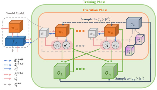
Figure 1.
MIRA framework.
- The world model of agent i (illustrated as the gray cubes in Figure 1) is trained using the data collected in the replay buffer in a supervised learning manner. This model consists of an environment dynamics model and opponent models represented as estimated policies of other agents . We introduce a hyperparameter H to determine the horizon of recursive reasoning for the world model.
- The latent-variable inference module (illustrated as a pewter cube) realizes the extraction of trajectory from historical data and records it into the replay buffer together with the experience at each time step within an episode. The accumulated off-policy data are transformed from past trajectory to a probability variable Z via the latent-variable inference module, which is resampled by a posterior probability (illustrated as a pewter solid arrow) on trajectory .
- The critic module and the actor module (described as the green cubes and the orange cubes, respectively) exploit the latent variable Z in reinforcement learning tasks; Z is a probabilistic variable that embeds the non-stationarity of the current environment and incorporates with the input vectors of in the training. The critic module is implemented by the Deep Q-learning network and essentially acts as a state-action value function. Moreover, the actor module denoted as updates the parameters via the policy gradient guided by the corresponding critic module.
During the execution phase, the agents work in a distributed fashion. When performing a given task at time step t, agent i obtains its corresponding observation . First, the observation will be input into the actor module and the world model. The agent policy along with opponent models produces imagined joint actions that makes one step rollout. It is noteworthy that the opponent models are a mapping as Equation (4):
from the observation of the modeller i rather than of the modelled agent j to the action . Second, the world model is reused H times to make multi-step rollouts. Meanwhile, the latent-variable inference module takes the imagined trajectory (marked as a gray dotted arrow) as the input to infer . In the k-th time of recursive reasoning, is updated as Equation (5).
Furthermore, the imagined joint action determined by z acts on the environment dynamics model to generate the imagined observation . After H recursive loops, an imagined trajectory is produced by the world model. Third, the latent-variable inference module constructs the latent variable Z and infers the value z by online probabilistic filtering of the rollouts for the downstream RL process. Combining with the , the inferred value is provided to the policies for decision making.
4.2. World Model
We design a world model as a cognitive model for each agent. After observing and trial-and-error in the objective world, it includes the knowledge learned by the agent about how the environment and other agents work and is used for inferring unknown information. After centralized training, the world model can predict the behaviors of other agents and reason the state transition of the environment. When executed alone, the world model is capable of generating a large number of imagined trajectories. These trajectories contain the agent’s knowledge about the current environment and are used for subsequent inference.
4.2.1. Modeling Environment Dynamics
Generally speaking, the environment dynamics model uses the current state s and action a as the condition to predict the transition to the next state . However, the observational field of agent i limits the acquisition of complete state information, so it is unreasonable to predict the environment state s from its perspective. Fortunately, the world model can facilitate the prediction of what the agent can observe, i.e., using existing observations and its own action a to predict the difference between the current observation and the next observation of the environment.
During the centralized training phase, we adopt a probabilistic ensemble network to learn the dynamics model based on the agent’s historical observations and actions stored in the experience replay buffer . Specifically, we train an ensemble of M probabilistic neural networks whose outputs parametrize a Gaussian distribution with diagonal covariance, formalized as Equation (6):
The ensemble of independently trained models helps to overcome the epistemic uncertainty of predictions; otherwise, a single neural network may misestimate by insufficient data training. The parameters of the ensemble model are optimized according to the loss function defined by [37], as shown below.
4.2.2. Reasoning Imagined Rollouts
We explicitly build opponent models to predict possible actions of other agents by assuming that all the agents have a similar architecture. Then, the opponent models are trained to generate behaviors by imitating the observations of the corresponding agents. The opponent models of agent i are represented as a parameterized stochastic policy , which is a multi-layer neural network for computing the action based on the current observation, i.e.,
The loss function of opponent models consists of two terms: (1) A Kullbach–Leibler divergence between the ground-truth action of the observed agent and the output of opponents models. (2) An entropy of is used to increase the diversity of the opponent policy. Specifically, the loss function is written as
where stands for a coefficient that balances model exploitation and exploration.
With both the environment dynamics model and opponent models, the role of the world model is to play rollouts between the agent and the opponent model. As illustrated in Figure 2, the rollouts policy is executed by the agent i like the gray triangles, and the imagined actions of other agents are produced by like the blue triangles. In the beginning, an observation is perceived by agent i in the real world, sending it to the world model. After H-step rollout, the world model eventually produces an imagined trajectory with a fixed length: .
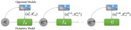
Figure 2.
Imagined rollouts.
4.3. Latent-Variable Inference Module
In this subsection, we first introduce two specific features of POSGs that make meta-learning applicable and analyze the factors that lead to the non-stationarity problem. Thereafter, we propose an elegant method to use the past experience to estimate the uncertainty of the task during module training and to infer a latent variable Z that encapsulates uncertain information of the current task with the posterior probability during module testing. We estimate the posterior probability using variational inference as an approximation and sample z that explores the non-stationarity of the environment to solve a task. In addition, the method to apply the latent variable in the downstream RL tasks is introduced as well.
Each task in meta-RL methods [16,38] is a particular MDP noted as and follows a distribution . In a POSG, task is performed independently by agent i with its partial observations and the task can therefore be seen as a Partially Observed MDP (POMDP), denoted as . The POSG has two characteristics that motivate us to apply meta-learning to it. First, the partial observability prevents the agent from obtaining complete environmental information, so that the policy of an agent depends on its own observation of the external environment instead of the global real state of the environment. Second, the distribution of the current task is affected by the policy of opponents. When other agents adaptively change their policies, it will lead to a different and results in a new task distribution . In such cases where the MDP cannot be guaranteed to be stable, it is known that it is difficult for RL to learn the optimal policies. To this end, meta-learning is applied to infer the uncertain information of the current task in order to make the algorithm adapt to different task distributions.
Specifically, a task includes initial state distribution , transition probability , emission probability , and reward function . The policies of other agents are changing over time in possible ways including goal switching and policy adaption, which leads to the uncertainty of . Hence, the non-stationarity of the environment encompasses with varying observation function , which can be regarded as different task distributions and in MDPs in different time steps.
For adaption to these different distributions, the meta-training process learns to reason about knowledge of the current task based on experiences of previous tasks. Because the task is performed consistently, the MDP transitions in an episode have temporal dependencies. Therefore, the method of inferring task knowledge does not depend on a single state s but is supposed to take into account the MDP transitions. To this end, we collect multiple trajectories in every single episode as the task experiences. These trajectories contain the elements of the MDP transitions that implied the uncertainty over this task.
To explicitly represent the salient information of the current environment, a probabilistic latent variable Z is constructed via the posterior probability distribution . The probability distribution form of p is not known anyway. Instead, we can approximate it by another posterior probability distribution by a variational inference approach, where q can be any form of distribution. This article formalizes the variational posterior as a Gaussian distribution.
The approximation of distribution p is achieved by solving an optimization problem, i.e., maximizing the evidence lower bound (ELBO) to ensure accurate inference. Specifically, we use an LSTM-based encoder to generate the posterior distribution of the latent variable Z. LSTM is a recurrent neural network (RNN) with a memory storage function. By training model weights, RNN evaluates the hidden state of the environment and memorizes the information about the task. It is suitable for solving partial observation problems and can be well applied in meta-learning.
Note that to make the latent variable distribution more stable, we use the information bottleneck theory to guide the learning of the distribution parameter . A prior is set as the standard normal distribution to maximize the mutual information about the latent variable in the compressed trajectories. In the design of the loss function shown as Equation (10), it is hoped that the distribution q will not deviate too far from the prior one.
The proposed algorithm combines the inferred value z of the latent variable, which embeds the useful knowledge to infer the current task, and some explicitly given information, such as observations and actions of agents, so that it can effectively mitigate the impact of environmental non-stationarity. The next subsection will reveal how to evaluate the state-action value on the basis of z and guide the policy to select the optimal action.
4.4. Implementation on Off-Policy Reinforcement Learning
We address how meta-learning can be performed for non-stationary environments on off-policy RL algorithms in this subsection. The proposed approach is implemented on the basis of the multi-agent soft actor-critic (SAC) algorithm [10], where each agent has a set of actor-critic functions approximated by MLP networks. The SAC algorithm is a sample-efficient off-policy RL algorithm, which balances stability and utilization by introducing the entropy of the policy distribution into the objective function. The stochastic policies adopted by SAC can integrate well with the probabilistic latent variable.
The training phase of our approach is detailed in Algorithm 1. First, the components in the proposed method are initialized, including a replay buffer, an encoder, an ensemble environment dynamics model, and opponent models in the world model (lines 1 to 2). Furthermore, a pair of actor-critic models are defined for each agent as MLP networks (line 3). Second, the imagined trajectory is generated in the world model (lines 4 to 7) and the policy is executed on the inferred value z (lines 8 to 9). Third, the experiences within an episode are collected. A sampler generates trajectory at time step t from and stores it in the buffer together with for model training (line 11). The parameters of the environment dynamics model are updated and an optimization term for a latent-variable inference module is defined (lines 13 to 14). Subsequently, the components of each agent, including the actor networks, opponent models, critic networks, and inference modules, are updated (lines 16 to 18). Via a graph model, the inference module updates its parameters by the back propagation of the critic and the encoder (line 19).
| Algorithm 1 Centralized training. |
| Parameter: Learning rate , rollout length H. Output: Actor networks and critic networks
|
The critic network is used to approximate the soft Q-function by minimizing the soft Bellman residuals to train the network parameters as Equation (11):
The Q-value function is evaluated through the target critic network with frozen parameters, which is synchronized with the update rate after a period of steps. The implementation can be achieved by optimizing the stochastic gradient as Equation (12):
where is an auto-tuning temperature parameter specified in the SAC algorithm with a given target entropy. The actor module uses a stochastic policy; its optimization objective is given in Equation (13):
The critic network evaluates the state-action value of the agent’s strategy based on the current state and the joint actions . Using the complete information about the environment, the critic can guide the policy parameters to be updated to a higher value gradient and help the actor learn the strategy to obtain higher rewards. The loss function of the actor is given in Equation (14):
Algorithm 2 describes the specific process of the meta-test. After training with a large amount of empirical data, MIRA can avail the world model for online reasoning and use the latent-variable inference module to infer representation for the current policy. The agent expands the imagined rollout (lines 2 to 6) according to the observation and uses the inference module to obtain the value of a probability variable to augment the input of the policy network (lines 7 to 8).
| Algorithm 2 Decentralized executing. |
Input: Actor networks and critic networks .
|
5. Empirical Evaluation
In this section, we evaluate the performance of the proposed method MIRA and analyze its properties comprehensively. In Section 5.1, we introduce the experimental platform MPE and several competing baselines to be compared. In Section 5.2, we evaluate the performance of MIRA and the CTDE-based counterparts in two scenarios in MPE in terms of their sampling efficiency and finally gained rewards in training. Subsequently, we further conduct ablation experiments to test how latent-variable-based policies and information-bottleneck-optimized posterior distributions can improve the fast adaptation of MIRA to changing tasks. Finally, we explore the impact of the rollout horizon H in the world model, the most important hyperparameter in MIRA, on the performance of the proposed approach.
5.1. Experimental Settings
5.1.1. Experimental Environment
We select the Multiagent Particle Environments (MPE) as the benchmark suite for our experiments. The MPE experimental scenarios first appeared in the work of [39] to specify cooperative and competitive tasks among multiple particles. There are continuous state spaces in these scenarios, where both continuous or discrete actions are allowed. An agent in the environment obtains partial observations, including its absolute velocity, relative position, and relative velocity to other entities. In this article, we test the competing algorithms in two typical scenarios in MPE, as described below.
Predator-prey. In this scenario, a group of predators (larger particles in Figure 3a) attempt to capture the fleeing prey (the small particle in Figure 3a) while avoiding the obstacles (black circles), with a positive payoff when the locations of at least one predator and the prey overlap. An agent can perceive its own absolute position, velocity, and relative velocity and position to obstacles and other agents. We train multiple agents as the predators to cooperatively hunt the escaping prey through this scenario.
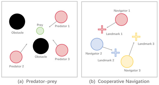
Figure 3.
An example of the MPE benchmark. (a) Three predators try to capture prey to obtain rewards. (b) Three navigators aim for reaching the nearest landmarks.
Cooperative Navigation. This scenario specifies a cooperative task where there are N agents (shown as circles in Figure 3b), and the same number of destinations (illustrated as addition signs in Figure 3b). The goal for an agent is to navigate to the destination as near as possible, and the distance between the agent and the nearest destination is used as a negative reward given by the environment. An agent can perceive its absolute position, velocity, and relative position to obstacles and other agents. Therefore, this task requires each agent to learn to coordinate with teammates to get as close to the landmark as possible but avoid multiple agents heading to the same destination.
5.1.2. Baselines
We select four CTDE-based algorithms as competing baselines to compare the performance of MIRA against them.
COMA [21]: An on-policy MARL method with an actor-critic architecture. COMA uses the critic module to calculate a counterfactual baseline that marginalizes an action of a single agent. This counterfactual baseline works as an advantage function for updating the actor module, which is beneficial to the credit assignment of the agent.
MAAC [4]: A modified version of COMA with a newly added attention mechanism. In its critic module, the attention mechanism is adopted to weight the information from other agents. The method of the actor module draws on the COMA algorithm, which adopts the multi-agent advantage function update.
MADDPG [5]: An off-policy MARL method based on the Deep Deterministic Policy Gradient algorithm. MADDPG uses global information to train the critic modules and learn actor modules based on the local information.
VDN [19]: A credit assignment MARL method that additively decomposes the state-action value (Q value) to improve the overall cooperation level of agents. We modify the action space of the environment so that VDN can use the Q value to select appropriate actions from a limited action space in the discretized environment.
5.2. Performance Evaluation
5.2.1. Overall Results
We first compare the overall performance of algorithms in each scenario, in which the total number of steps in each episode is limited to 25. The MPE environment is reset at the end of episodes and the initial positions of the agents and landmarks are then randomly initialized. The experiments are repeated five times independently for statistical results in each scenario. For the fairness of the comparison, these five algorithms are consistent in implementation. Five random seeds are selected identically for each method, and the actor-critic modules are implemented by similar MLP networks. Moreover, we set the same hyperparameters in all algorithms, including the learning rate, discount factor, hidden layer size, and target network update rate. Their values are shown in Table 1 for detail. In addition, we define two metrics for performance evaluation:

Table 1.
Hyperparameters Set.
- Convergence Reward (CR): The mean value of the episode reward in the last 100 episodes, used as the convergence result of the algorithms.
- Convergence Duration (CD): The number of training episodes required for the episode reward to stabilize within of the convergent reward.
The rollout length H of the MIRA algorithm is fixed to 5 and the prey adopts a policy of random actions in the predator-prey scenario. Figure 4 shows the episode reward curves of all the five methods when training on the predator-prey scenario, where the y-axis represents the accumulated rewards for all agents in an episode. The plot is smoothed using a one-dimensional Gaussian filter with , where the bold lines and the corresponding shaded areas represent the mean values and upper-lower bounds of the episode rewards over the five repeated but independent runs, respectively. After training episodes, all algorithms reached their policy convergence. Figure 4 shows that the curves of COMA, MADDPG, and VDN are similar, and the episode reward of MAAC increases more slowly than other competitors. MIRA improves much faster than the others and stabilizes at a considerably higher value.
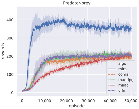
Figure 4.
The training process of MIRA and four CTDE baselines on the predator-prey benchmark.
The evaluation results of the metrics in the predator-prey case are shown in Table 2. The overall performance of MIRA is substantially better than other compared algorithms. To be specific, its convergence reward is 1.7–2 times as large as those of other algorithms and MIRA requires 2.7–7.5 episodes less than all its counterparts to reach its convergence. It is believed that the setting where the prey adopts random actions leads the environment to feature inherent non-stationarity in the sense that the pre-train policies for cooperation make it difficult to tackle uncertain tasks. We argue that MIRA works for the reason that it is specially designed for non-stationary environments. In MIRA, the world model learns to rollout independently, and the inference module learns the distribution of the latent variable Z through variational approximation and samples the value z from the posterior to explore non-stationarity, which is integrated into the model-free RL framework. Therefore, MIRA not only learns to predict future trajectories from historical experience but also uses the predictions to infer current task characteristics to help make better decisions. In contrast, other algorithms rely on centralized training to reach cooperative consensus and cannot infer the task independently during distributed execution. When faced with non-stationary tasks, such as environmental changes, it is difficult for their policies to perform as well as they do during training.
Table 2.
Convergence performance of evaluated algorithms on predator-prey.
Figure 5 shows the results of the five algorithms on the Cooperative Navigation scenario, where the curves are smoothed using a one-dimensional Gaussian filter with . All algorithms are trained for episodes. It can be seen that the curve of MIRA has a sharp trend of convergence. The reward obtained by MIRA remains stable at a much higher level only after episodes, whereas other algorithms tend to converge after episodes. As shown in Table 3, MIRA has 2.8–3 times faster convergence speed and 10–16% better asymptotic performance than other algorithms. It is shown that MIRA is not only competent for multi-agent competitive tasks but also has comparable performance to other algorithms in multi-agent cooperative tasks. Although model-free CTDE methods can also learn to cooperate well tardily, MIRA can improve their learning speed and performance by increased exploration via a latent variable.
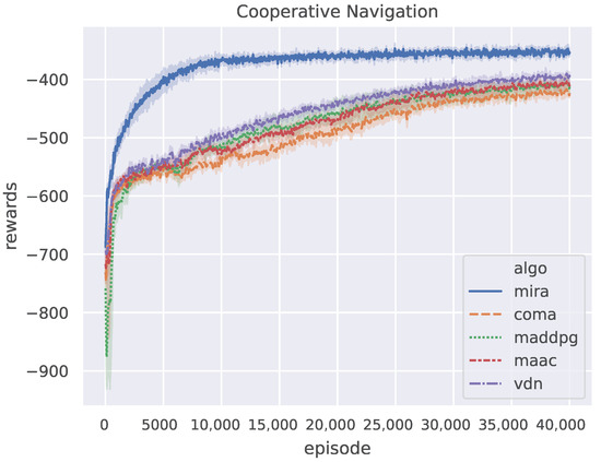
Figure 5.
The performance of MIRA and four CTDE baselines on the Cooperative Navigation benchmark.
Table 3.
Convergence performance of evaluated algorithms on Cooperative Navigation.
Generally speaking, different from the model-free baselines that merely use experiences to update policies, MIRA trains the world models that generate imagined trajectories to work more effectively. The latent variable Z generated according to these trajectories can vastly enhance the representation ability of agent policy. The agent based on MIRA generates a family of policy functions and determines the policy according to the value of z, so that the agent policy can be fully explored and the efficiency of MIRA is improved. However, those agents based on the other methods lack the ability to cope with non-stationarity when faced with an observation and treat the policy as a deterministic action distribution.
5.2.2. Ablation Studies
We set up four ablation versions of the proposed method to analyze the reasons for the improvement of our algorithm performance and demonstrate the effects of individual modules in MIRA. Among them:
- MIRA-w is a model-free MARL method without the world model and is taken as the baseline of other methods.
- MIRA-q adopts an LSTM network as a part of the actor module and processes the trajectory into a real-valued representation instead of an estimate on distribution .
- MIRA-i uses a latent-variable inference module to enhance policy exploration by posterior sampling and learn the posterior probability of a given input trajectory by maximizing the expected return from the critic modules. However, the loss function of its inference module eliminates the design of an information bottleneck for comparison with MIRA.
MIRA has an additional optimization formula Equation (10) in the design of the loss function for the inference module where the optimization of information bottleneck item tries to complete the task through a simpler standard normal distribution and obtain better generalization performance. Table 4 clearly summarizes the differences between the ablation algorithms and MIRA.
Table 4.
Comparison of ablation versions of the proposed method.
Figure 6 demonstrates the performance between our method and the ablation methods with different design mechanisms. As can be seen in Figure 6a, the sample efficiency of MIRA-q is far worse than that of MIRA and MIRA-i. One possible reason is that MIRA-q adopts a real-valued estimation instead of a probability distribution for the latent variable. The direct inference for each trajectory sample results in a very large variance on z, which is not only difficult to effectively explore policies under non-stationarity but useless for decision making (even worse than MIRA-w). This also shows that directly estimating the latent variable through learning representation methods cannot bring about significant improvement. Both MIRA-i and MIRA have the latent-variable inference modules that estimate z from the sampling posterior distribution. The corresponding curves in Figure 6a indicate the excellent sample efficiency of the inference modules. We attribute this effect to the posterior sampling on Z that enhances the ability of policies to explore non-stationarity and leads to better performance. Furthermore, the variational approximation of the information bottleneck in the loss function constrains to carry the mutual information between Z and trajectories at most. Therefore, z contains task information indicating non-stationarity to the greatest extent, which enables MIRA to have better convergent results than MIRA-i.
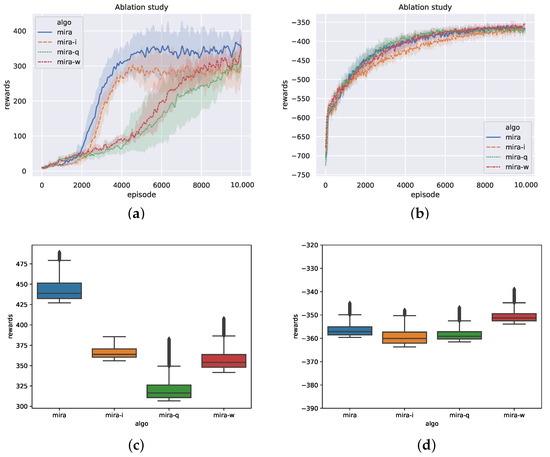
Figure 6.
Performance of ablation versions. (a) Training curves on predator-prey. (b) Training curves on Cooperative Navigation. (c) Ending rewards on predator-prey. (d) Ending rewards on Cooperative Navigation.
In Figure 6c,d, we sample the episode rewards of the four methods after convergence and plot the distribution of evaluation results in the boxplot. From Figure 6c, it can be seen that the episode reward distributions of MIRA-w and MIRA-q are scattered and have much more outliers. The episode rewards of MIRA are higher than the other three, and the policy performance is more stable.
Cooperative Navigation is a contrasting example. In Figure 6d, the episode rewards of the above methods are not very different, and all the sample distributions are stable. In the fully cooperative scenario, the uncertainty is eliminated by sharing information among the agents, thus better solving the non-stationarity problem. In conclusion, the MIRA method not only outperforms other methods in competitive scenarios but also maintains stable performance in cooperative scenarios.
5.2.3. Opponent Loss
To analyze the accuracy of the world model, we treat the convergence of the loss function as the metric for evaluating the training performance. In our examples, the MIRA algorithm is set with and we test the loss value of the opponent models in the predator-prey and Cooperative Navigation scenarios, respectively. The training curve of predator-prey scenario is shown in Figure 7. The results show that after short-term training, the model loss can be stably converged, and the opponent model can quickly learn the task that predicts the actions of corresponding agent. Figure 8 shows the model loss training curve in the Cooperative Navigation scenario. It can be seen that the loss values of the three agents roughly coincide and converge approximately, which indicates the realization of the prediction task. However, all these models suffer from inevitable errors due to the limited approximation ability of deep neural networks for policies function and the continuous changes of learning targets i.e., the real opponent policies.
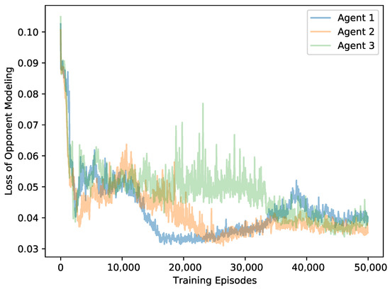
Figure 7.
The loss curves of opponent models on predator-prey.
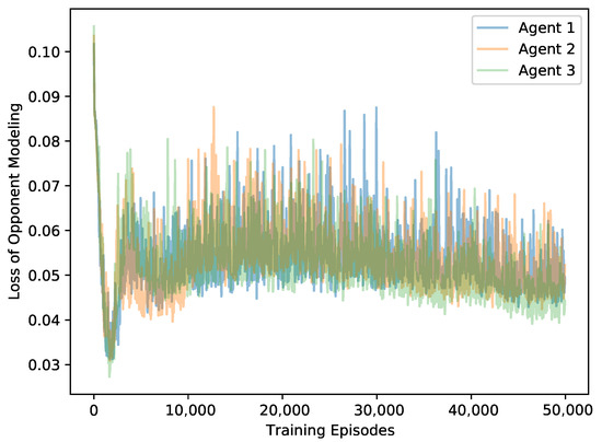
Figure 8.
The loss curves of opponent models on Cooperative Navigation.
5.2.4. Hyperparameter Test
The recursive reasoning horizon H in the world model is an artificially determined hyperparameter that changes the length of the trajectory input to the latent-variable inference module. Because the imagined trajectories of a task are particularly important for MIRA, we explore how the length of the imagined rollout affects performance. In previous experiments, we set the default value . In this subsection, we set up four control groups in the predator-prey scenario: rollout lengths and an extreme long set of lengths , with five replicates for each group. The reward curves of the baseline algorithm and MIRA for different rollout lengths are depicted in Figure 9.
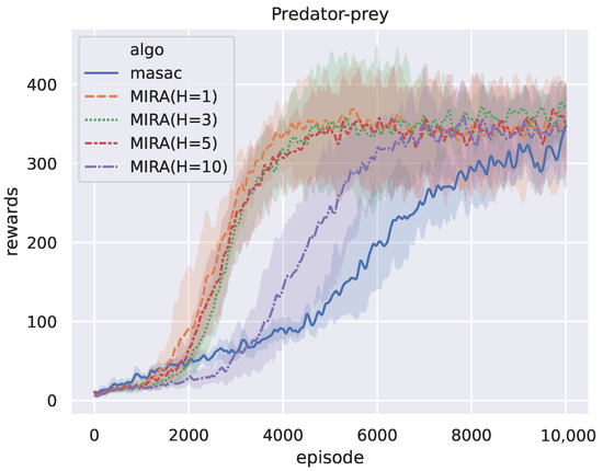
Figure 9.
MIRA training curves for various values of the rollout length.
The figure shows that the difference between the trajectory length H has a limited effect on the final performance of MIRA, whereas the number of episodes for MIRA with to reach the final performance is significantly larger. We report the Convergence Rewards and Convergence Durations of different settings of trajectory lengths in Table 5. Compared with the experimental group of , the CRs of groups and increase by and , respectively. At the same time, the training CDs delay by and . It is worth noting that the group of is inferior to the other groups, especially in CD, and the results reflect that an excessively long trajectory length leads to lower sample efficiency, which is counterintuitive. In response to this phenomenon, one potential explanation is that due to the inherent error of the world model, as the number of recursive reasoning steps increases, the predicted environment dynamics gradually shift away from the ground truth and therefore the decision making on actions will gradually accumulate errors. As a result, the first few steps of the imagined rollouts are more accurate and the help for inference on the latent variable is obvious, whereas the subsequent rollouts generate invalid redundancy. However, the MIRA method outperforms its baseline MASAC for all rollout lengths. In conclusion, the hyperparameter H should be controlled within a reasonable range to ensure sample efficiency while optimizing the final performance.
Table 5.
Convergence performance for different trajectory lengths.
6. Conclusions
In this article, we propose a novel imagined rollouts augmented strategy for accommodating the non-stationarity problem in multi-agent reinforcement learning. We first establish a world model for inferring the environment dynamics and modeling the actions of opponents and propose a method of using model rollouts to generate imagined trajectories. Based on the acquisition of imagined trajectories, we introduce a latent-variable inference module for policy exploration, which helps the agent learn the representation of the environmental non-stationarity by establishing trajectory-based inference. Experimental results show that our method is significantly sample-efficient and outperforms other MARL benchmarks on the MPE testbed. A set of ablation experiments prove that the meta-learning method with the latent variable effectively enhances policy exploration under non-stationarity and greatly improves the convergence speed of the policy.
In future work, we consider the following two improvements. First, due to the potential error between the world model and the real environment, the imagined trajectory may deviate from the real trajectory as the rollout length increases. We will further study the theoretical error bound of the world model and propose methods to control the error by self-adjusting the rollout length H. Second, we will consider cooperation and confrontation with types of agents based on manual rules and heuristic algorithms and study the rapid adaptability in heterogeneous multi-agent systems.
Author Contributions
H.X. proposed the methodology, performed the experimental evaluation, and prepared the manuscript. Q.F. analyzed and validated the feasibility of the methodology. C.H. provided the formal analysis and edited the manuscript. Y.H. reviewed, edited, and revised the manuscript. This manuscript was finished under the supervision of Q.Y. All authors have read and agreed to the published version of the manuscript.
Funding
This work was supported in part by the National Natural Science Foundation of China under Grant 61273300, 62102432, 62103420, 62103428, and 62103425, the Natural Science Fund of Hunan Province under Grant 2021JJ40697 and 2021JJ40702 and the Youth Science Fund of National Natural Science Foundation of China under Grant 62103420.
Institutional Review Board Statement
Not applicable.
Informed Consent Statement
Not applicable.
Data Availability Statement
Not applicable.
Conflicts of Interest
The authors declare no conflict of interest.
References
- Perrusquía, A.; Yu, W.; Li, X. Multi-agent reinforcement learning for redundant robot control in task-space. Int. J. Mach. Learn. Cybern. 2021, 12, 231–241. [Google Scholar] [CrossRef]
- Palanisamy, P. Multi-agent connected autonomous driving using deep reinforcement learning. In Proceedings of the 2020 International Joint Conference on Neural Networks (IJCNN), Glasgow, UK, 19–24 July 2020; IEEE: Piscataway, NJ, USA, 2020; pp. 1–7. [Google Scholar]
- You, X.; Li, X.; Xu, Y.; Feng, H.; Zhao, J.; Yan, H. Toward Packet Routing With Fully Distributed Multiagent Deep Reinforcement Learning. IEEE Trans. Syst. Man Cybern. Syst. 2022, 52, 855–868. [Google Scholar] [CrossRef]
- Iqbal, S.; Sha, F. Actor-Attention-Critic for Multi-Agent Reinforcement Learning. In Proceedings of the 36th International Conference on Machine Learning (ICML 2019), Long Beach, CA, USA, 9–15 June 2019; Chaudhuri, K., Salakhutdinov, R., Eds.; PMLR: New York, NY, USA, 2019; Volume 97, pp. 2961–2970. [Google Scholar]
- Lowe, R.; WU, Y.; Tamar, A.; Harb, J.; Pieter Abbeel, O.; Mordatch, I. Multi-Agent Actor-Critic for Mixed Cooperative-Competitive Environments. In Proceedings of the Advances in Neural Information Processing Systems 30: Annual Conference on Neural Information Processing Systems 2017 (NeurIPS 2017), Long Beach, CA, USA, 4–9 December 2017; Guyon, I., Luxburg, U.V., Bengio, S., Wallach, H., Fergus, R., Vishwanathan, S., Garnett, R., Eds.; Curran Associates, Inc.: Red Hook, NY, USA, 2017; pp. 6379–6390. [Google Scholar]
- Rashid, T.; Samvelyan, M.; de Witt, C.S.; Farquhar, G.; Foerster, J.N.; Whiteson, S. QMIX: Monotonic Value Function Factorisation for Deep Multi-Agent Reinforcement Learning. In Proceedings of the 35th International Conference on Machine Learning (ICML 2018), Stockholm, Sweden, 10–15 July 2018; PMLR: New York, NY, USA, 2018; Volume 80, pp. 4292–4301. [Google Scholar]
- Son, K.; Kim, D.; Kang, W.J.; Hostallero, D.E.; Yi, Y. QTRAN: Learning to Factorize with Transformation for Cooperative Multi-Agent Reinforcement Learning. In Proceedings of the 36th International Conference on Machine Learning (ICML 2019), Long Beach, CA, USA, 9–15 June 2019; Chaudhuri, K., Salakhutdinov, R., Eds.; PMLR: New York, NY, USA, 2019; Volume 97, pp. 5887–5896. [Google Scholar]
- Kuba, J.G.; Chen, R.; Wen, M.; Wen, Y.; Sun, F.; Wang, J.; Yang, Y. Trust Region Policy Optimisation in Multi-Agent Reinforcement Learning. In Proceedings of the ICLR 2022: The Tenth International Conference on Learning Representations, Online, 25–29 April 2022; Available online: https://arxiv.org/abs/2109.11251 (accessed on 21 January 2022).
- Wen, M.; Kuba, J.G.; Lin, R.; Zhang, W.; Wen, Y.; Wang, J.; Yang, Y. Multi-Agent Reinforcement Learning is a Sequence Modeling Problem. arXiv 2022, arXiv:2205.14953. [Google Scholar]
- Willemsen, D.; Coppola, M.; de Croon, G.C.H.E. MAMBPO: Sample-efficient multi-robot reinforcement learning using learned world models. In Proceedings of the IEEE/RSJ International Conference on Intelligent Robots and Systems (IROS 2021), Prague, Czech Republic, 27 September–1 October 2021; IEEE: Piscataway, NJ, USA, 2021; pp. 5635–5640. [Google Scholar]
- Zhang, W.; Wang, X.; Shen, J.; Zhou, M. Model-based Multi-agent Policy Optimization with Adaptive Opponent-wise Rollouts. arXiv 2021, arXiv:2105.03363. [Google Scholar]
- Sutton, R.S. Integrated Modeling and Control Based on Reinforcement Learning and Dynamic Programming. In Proceedings of the NIPS 1990, Denver, CO, USA, 26–29 November 1990. [Google Scholar]
- Wang, T.; Gupta, T.; Mahajan, A.; Peng, B.; Whiteson, S.; Zhang, C. RODE: Learning Roles to Decompose Multi-Agent Tasks. arXiv 2021, arXiv:2010.01523. [Google Scholar]
- Wang, T.; Dong, H.; Lesser, V.R.; Zhang, C. ROMA: Multi-Agent Reinforcement Learning with Emergent Roles. arXiv 2020, arXiv:2003.08039. [Google Scholar]
- Ribeiro, J.G.; Martinho, C.; Sardinha, A.; Melo, F.S. Assisting Unknown Teammates in Unknown Tasks: Ad Hoc Teamwork under Partial Observability. arXiv 2022, arXiv:2201.03538. [Google Scholar]
- Rakelly, K.; Zhou, A.; Finn, C.; Levine, S.; Quillen, D. Efficient Off-Policy Meta-Reinforcement Learning via Probabilistic Context Variables. In Proceedings of the 36th International Conference on Machine Learning (ICML 2019), Long Beach, CA, USA, 9–15 June 2019; PMLR: New York, NY, USA, 2019; Volume 97, pp. 5331–5340. [Google Scholar]
- Luo, Y.; Xu, H.; Li, Y.; Tian, Y.; Darrell, T.; Ma, T. Algorithmic Framework for Model-based Deep Reinforcement Learning with Theoretical Guarantees. In Proceedings of the 7th International Conference on Learning Representations (ICLR 2019), New Orleans, LA, USA, 6–9 May 2019; Available online: https://openreview.net/forum?id=BJe1E2R5KX (accessed on 17 December 2018).
- Tishby, N.; Pereira, F.C.N.; Bialek, W. The information bottleneck method. In Proceedings of the 37th Allerton Conference on Communication and Computation, Monticello, NY, USA, 22–24 September 1999; pp. 368–377. [Google Scholar]
- Peter Sunehag, G.L.; Gruslys, A.; Czarnecki, W.M.; Zambaldi, V.F.; Jaderberg, M.; Lanctot, M.; Sonnerat, N.; Leibo, J.Z.; Tuyls, K.; Graepel, T. Value-Decomposition Networks For Cooperative Multi-Agent Learning Based On Team Reward. In Proceedings of the 17th International Conference on Autonomous Agents and MultiAgent Systems (AAMAS 2018), Stockholm, Sweden, 10–15 July 2018; International Foundation for Autonomous Agents and Multiagent Systems: Richland, SC, USA, 2018; pp. 2085–2087. [Google Scholar]
- Lillicrap, T.P.; Hunt, J.J.; Pritzel, A.; Heess, N.; Erez, T.; Tassa, Y.; Silver, D.; Wierstra, D. Continuous control with deep reinforcement learning. In Proceedings of the 4th International Conference on Learning Representations (ICLR 2016), San Juan, Puerto Rico, 2–4 May 2016. [Google Scholar]
- Foerster, J.; Farquhar, G.; Afouras, T.; Nardelli, N.; Whiteson, S. Counterfactual multi-agent policy gradients. In Proceedings of the 32nd AAAI Conference on Artificial Intelligence (AAAI-18), New Orleans, LA, USA, 2–7 February 2018; AAAI Press: Palo Alto, CA, USA, 2018; Volume 32, pp. 2974–2982. [Google Scholar]
- Sukhbaatar, S.; Szlam, A.; Fergus, R. Learning Multiagent Communication with Backpropagation. In Proceedings of the Advances in Neural Information Processing Systems 29: Annual Conference on Neural Information Processing Systems 2016 (NeurIPS 2016), Barcelona, Spain, 5–10 December 2016; Lee, D., Sugiyama, M., Luxburg, U., Guyon, I., Garnett, R., Eds.; Curran Associates, Inc.: Red Hook, NY, USA, 2016; pp. 2244–2252. [Google Scholar]
- Das, A.; Gervet, T.; Romoff, J.; Batra, D.; Parikh, D.; Rabbat, M.; Pineau, J. TarMAC: Targeted Multi-Agent Communication. In Proceedings of the 36th International Conference on Machine Learning (ICML 2019), Long Beach, CA, USA, 9–15 June 2019; Chaudhuri, K., Salakhutdinov, R., Eds.; PMLR: New York, NY, USA, 2019; Volume 97, pp. 1538–1546. [Google Scholar]
- Mao, H.; Gong, Z.; Zhang, Z.; Xiao, Z.; Ni, Y. Learning Multi-agent Communication under Limited-bandwidth Restriction for Internet Packet Routing. arXiv 2019, arXiv:1903.05561. [Google Scholar]
- Kim, W.; Park, J.; Sung, Y. Communication in Multi-Agent Reinforcement Learning: Intention Sharing. In Proceedings of the 9th International Conference on Learning Representations (ICLR 2021), Vienna, Austria, 3–7 May 2021; Available online: https://openreview.net/forum?id=qpsl2dR9twy (accessed on 8 January 2021).
- Grover, A.; Al-Shedivat, M.; Gupta, J.K.; Burda, Y.; Edwards, H. Learning Policy Representations in Multiagent Systems. In Proceedings of the 35th International Conference on Machine Learning (ICML 2018), Stockholm, Sweden, 10–15 July 2018; Dy, J.G., Krause, A., Eds.; PMLR: New York, NY, USA, 2018; Volume 80, pp. 1797–1806. [Google Scholar]
- Papoudakis, G.; Christianos, F.; Albrecht, S. Agent Modelling under Partial Observability for Deep Reinforcement Learning. In Proceedings of the Advances in Neural Information Processing Systems 34: Annual Conference on Neural Information Processing Systems 2021 (NeurIPS 2021), Online, 6–14 December 2021; Ranzato, M., Beygelzimer, A., Dauphin, Y., Liang, P., Vaughan, J.W., Eds.; Curran Associates, Inc.: Red Hook, NY, USA, 2021; pp. 19210–19222. [Google Scholar]
- Racanière, S.; Weber, T.; Reichert, D.; Buesing, L.; Guez, A.; Jimenez Rezende, D.; Puigdomènech Badia, A.; Vinyals, O.; Heess, N.; Li, Y.; et al. Imagination-Augmented Agents for Deep Reinforcement Learning. In Proceedings of the Advances in Neural Information Processing Systems 30: Annual Conference on Neural Information Processing Systems 2017 (NeurIPS 2017), Long Beach, CA, USA, 4–9 December 2017; Guyon, I., Luxburg, U.V., Bengio, S., Wallach, H., Fergus, R., Vishwanathan, S., Garnett, R., Eds.; Curran Associates, Inc.: Red Hook, NY, USA, 2017; pp. 5690–5701. [Google Scholar]
- Rusu, A.A.; Rao, D.; Sygnowski, J.; Vinyals, O.; Pascanu, R.; Osindero, S.; Hadsell, R. Meta-Learning with Latent Embedding Optimization. In Proceedings of the 7th International Conference on Learning Representations (ICLR 2019), New Orleans, LA, USA, 6–9 May 2019; Available online: https://openreview.net/forum?id=BJgklhAcK7 (accessed on 18 December 2018).
- Duan, Y.; Schulman, J.; Chen, X.; Bartlett, P.L.; Sutskever, I.; Abbeel, P. RL2: Fast Reinforcement Learning via Slow Reinforcement Learning. In Proceedings of the 5th International Conference on Learning Representations (ICLR 2017), Toulon, France, 24–26 April 2017; Available online: https://openreview.net/forum?id=HkLXCE9lx (accessed on 21 February 2017).
- Yang, Y.; Wang, J. An Overview of Multi-Agent Reinforcement Learning from Game Theoretical Perspective. arXiv 2020, arXiv:2011.00583. [Google Scholar]
- Higuera, J.C.G.; Meger, D.; Dudek, G. Synthesizing Neural Network Controllers with Probabilistic Model-Based Reinforcement Learning. In Proceedings of the 2018 IEEE/RSJ International Conference on Intelligent Robots and Systems (IROS 2018), Madrid, Spain, 1–5 October 2018; IEEE: Piscataway, NJ, USA, 2018; pp. 2538–2544. [Google Scholar]
- Fu, J.; Levine, S.; Abbeel, P. One-shot learning of manipulation skills with online dynamics adaptation and neural network priors. In Proceedings of the 2016 IEEE/RSJ International Conference on Intelligent Robots and Systems (IROS 2016), Daejeon, Korea, 9–14 October 2016; IEEE: Piscataway, NJ, USA, 2016; pp. 4019–4026. [Google Scholar]
- Janner, M.; Fu, J.; Zhang, M.; Levine, S. When to Trust Your Model: Model-Based Policy Optimization. In Proceedings of the Advances in Neural Information Processing Systems 32: Annual Conference on Neural Information Processing Systems 2019 (NeurIPS 2019), Vancouver, BC, Canada, 8–14 December 2019; Wallach, H., Larochelle, H., Beygelzimer, A., d’Alché-Buc, F., Fox, E., Garnett, R., Eds.; Curran Associates, Inc.: Red Hook, NY, USA, 2019; pp. 12498–12509. [Google Scholar]
- Deisenroth, M.P.; Rasmussen, C.E. PILCO: A Model-Based and Data-Efficient Approach to Policy Search. In Proceedings of the 28th International Conference on Machine Learning (ICML 2011), Bellevue, WA, USA, 28 June–2 July 2011; Omnipress: Madison, WI, USA, 2011; pp. 465–472. [Google Scholar]
- Heess, N.; Wayne, G.; Silver, D.; Lillicrap, T.; Erez, T.; Tassa, Y. Learning Continuous Control Policies by Stochastic Value Gradients. In Proceedings of the Advances in Neural Information Processing Systems 28: Annual Conference on Neural Information Processing Systems 2015 (NeurIPS 2015), Montreal, Canada, 7–12 December 2015; Cortes, C., Lawrence, N., Lee, D., Sugiyama, M., Garnett, R., Eds.; Curran Associates, Inc.: Red Hook, NY, USA, 2015; pp. 2944–2952. [Google Scholar]
- Chua, K.; Calandra, R.; McAllister, R.; Levine, S. Deep Reinforcement Learning in a Handful of Trials using Probabilistic Dynamics Models. In Proceedings of the Advances in Neural Information Processing Systems 31: Annual Conference on Neural Information Processing Systems 2018 (NeurIPS 2018), Montréal, QC, Canada, 3–8 December 2018; Bengio, S., Wallach, H., Larochelle, H., Grauman, K., Cesa-Bianchi, N., Garnett, R., Eds.; Curran Associates, Inc.: Red Hook, NY, USA, 2018; pp. 4759–4770. [Google Scholar]
- Gupta, A.; Mendonca, R.; Liu, Y.; Abbeel, P.; Levine, S. Meta-Reinforcement Learning of Structured Exploration Strategies. In Proceedings of the Advances in Neural Information Processing Systems 31: Annual Conference on Neural Information Processing Systems 2018 (NeurIPS 2018), Montréal, QC, Canada, 3–8 December 2018; Bengio, S., Wallach, H., Larochelle, H., Grauman, K., Cesa-Bianchi, N., Garnett, R., Eds.; Curran Associates, Inc.: Red Hook, NY, USA, 2018; pp. 5307–5316. [Google Scholar]
- Mordatch, I.; Abbeel, P. Emergence of Grounded Compositional Language in Multi-Agent Populations. In Proceedings of the AAAI Conference on Artificial Intelligence, New Orleans, LA, USA, 2–7 February 2018; AAAI Press: Palo Alto, CA, USA, 2018; Volume 32, pp. 1495–1502. [Google Scholar]
Publisher’s Note: MDPI stays neutral with regard to jurisdictional claims in published maps and institutional affiliations. |
© 2022 by the authors. Licensee MDPI, Basel, Switzerland. This article is an open access article distributed under the terms and conditions of the Creative Commons Attribution (CC BY) license (https://creativecommons.org/licenses/by/4.0/).