Tourist Arrival Forecasting Using Multiscale Mode Learning Model

Abstract

The forecasting of tourist arrival depends on the accurate modeling of prevalent data patterns found in tourist arrival, especially for daily tourist arrival, where tourist arrival changes are more complex and highly nonlinear. In this paper, a new multiscale mode learning-based tourist arrival forecasting model is proposed to exploit different multiscale data features in tourist arrival movement. Two popular Mode Decomposition models (MD) and the Convolutional Neural Network (CNN) model are introduced to model the multiscale data features in the tourist arrival data The data patterns at different scales are extracted using these two different MD models which dynamically decompose tourist arrival into the distinctive intrinsic mode function (IMF) data components. The convolutional neural network uses the deep network to further model the multiscale data structure of tourist arrivals, with the reduced dimensionality of key multiscale data features and finer modeling of nonlinearity in tourist arrival. Our empirical results using daily tourist arrival data show that the MD-CNN tourist arrival forecasting model significantly improves the forecasting reliability and accuracy.

1. Introduction

As one of the cornerstones of the rapidly developing service economy, the tourism industry is intertwined with the development of different sectors of the economy. It is subject to the influences of a very complicated and diversified range of factors for different purposes over a different time horizon [1,2]. For example, key tourist motivations may include pleasure, business visiting, relatives, conferences, study, and others [3]. The long-term influencing factors may include macroeconomic policy adjustments. The short-term influencing factors may include weather, diseases, exchange rate changes, natural hazards, major recreation, sports events, changes in essential inputs, and trade barriers [4,5,6,7,8,9,10,11,12]. As these factors come and go over time, their joint influence on the tourist arrival determination process has resulted in an unstable and nonstationary tourist arrival changing process. It represents significant factors for the sustained development of the tourism industry, from tourism planning to budgeting. Various issues concerning different aspects of tourist arrival have attracted significant attention from academics, practitioners, and investors.

The tourism demand forecasting research has profound implications for both public and private parts of the economy [1]. The private or industrial sectors rely on accurate tourist demand forecasting for their efficient operations, i.e., they need accurate tourist forecasts to plan, set appropriate prices, recruit enough staff, and allocate sufficient resources to meet the tourism demand for products and services in the holiday season and under rapidly changing market circumstances. The public sectors, such as local governments, rely on accurate tourist demand forecasting for public policy formulation, transportation development, the promotion and development of specific tools, tourism industry, and related industrial development in the supply chain [13,14]. Developing a more accurate and reliable tourist arrival forecasting model is, therefore, very important for the efficient operation of the tourism industry and academic research [1,15].

The forecasting of tourist arrival and tourist demand has been a main research topic in the literature over the years [16,17]. Song and Li [16] presented a comprehensive survey on the early development of tourism demand forecasting. The mainstream tourism demand forecasting models are classified as either qualitative models, such as judgmental methods, or quantitative models, such as econometrics models, time series models, or other emerging models such as Artificial Intelligence (AI) models [14,16]. The structural econometrics model has been used to investigate the impacts of different influencing factors on tourist arrival. For example, Nguyen and Valadkhani [5] studied the sensitivity of the exchange rate to tourist arrival. The main problem with this approach is that the influencing factors of tourist arrivals are very complicated and diversified. It is difficult to identify these influencing factors exactly with high accuracy, not to mention the modeling of the relationship between these influencing factors and tourist arrival. In the meantime, another popular approach is the time series approach, which extracts patterns from the analysis of the historical observation and current value of tourist arrival, and ultimately tries to infer the future changes [18]. Mainstream time series models such as the Autoregressive Integrated Moving Average (ARIMA) model, Seasonal ARIMA, Generalized Autoregressive Conditional Heteroskedasticity (GARCH) model, Exponential Smoothing (ETS), Naive, etc. have been developed to capture some of the most widely acknowledged data patterns in the tourist demand forecasting literature such as autocorrelation, volatility clustering, and seasonality [16,19]. Aside from these approaches, the tourism demand forecasting literature has paid increasing attention to the potential of Artificial Intelligence and Machine Learning models to capture and model the nonlinear data features in tourist arrivals with an assumption-free and data-driven approach [20]; typical models include Neural Networks and Support Vector Regression [21]. For example, Cang [22] found that the neural network and support vector regression-based combination model achieves the best forecasting accuracy compared to the individual models. However, the neural network is known to suffer from the overfitting problem, especially when it is applied to a small sample size, such as low-frequency data. In recent years, Deep Learning, as one of the latest developments in the field, has brought much hope and been widely applied in the economics and finance field [23,24]. It has become more and more popular in the tourism research literature [13,25,26,27]. For example, Lawet al. [25] proposed a bagging-based multivariate simple deep learning model to forecast the monthly tourist arrival. It is constructed based on individual models such as stacked autoencoder and the kernel-based extreme learning machine. It refers to a collection of rapidly developing models in the Artificial Intelligence field, such as Convolutional Neural Network (CNN) and Long Short-Term Memory (LSTM) [28,29,30,31,32]. Songet al. [17] provided an updated comprehensive review on the latest developments in tourism demand forecasting. It is interesting to see how the focus of the tourism demand forecasting models has gradually shifted from the mostly econometric and time series approach to the more recent artificial intelligence and data analysis model.

Until now, no consensus on the optimal tourist arrival forecasting model has been reached in the literature after years of development [20,33,34]. The rich set of data features in the tourist arrival data at higher frequency and larger sample size would lead to exponential increasing level of model risk and lower level of generalization in forecasting, which has brought new challenges as well as opportunities for better tourist arrival modeling and forecasting [14]. When modeling and analysis are performed at a much shorter time scale, such as at the daily or intraday frequency, many different data characteristics such as seasonality, autocorrelation, multiscale, etc. may prevail, with the disruptions of transient or extreme factors [6,10]. Among the newly emerging data characteristics, the multiscale data feature is one of the most important and promising data features. The multiscale data feature is widely found in natural and economic systems, such as energy markets and exchange markets. Motivations for tourist travel decisions and tourist destination supply also vary with different time horizon focuses and budget scales, which results in the multiscale characteristics in the tourist arrival changes. However, in the tourist arrival forecasting and tourism management literature, the modeling of multiscale data features has only received limited attention.

To model the multiscale data characteristics, there have been two interesting developments in the recent literature. Firstly, multiscale data decomposition models such as Empirical Mode Decomposition (EMD) and Variational Mode Decomposition (VMD) have received increasing attention in tourism demand forecasting [35,36,37,38]. For example, Xing et al. [37] proposed an adaptive multiscale ensemble model that combines VMD with the ARIMA, SARIMA, and LSSVR models; it models data features such as trend and seasonality to produce tourist arrival forecasts with improved accuracy. Xie et al. [38] combined Complete Ensemble EMD with Adaptive Noise (CEEMDAN) with Elman’s neural network model to enhance the predictive accuracy of tourist arrival forecasts. Between EMD and VMD models, EMD has been known to suffer from the inherent mode mixing issue, which poses difficulty to its estimation accuracy. As its name implies, the mode mixing problem refers to the fact that the supposedly unique intrinsic modes may share common characteristics and demonstrate similar data patterns, making them indistinguishable from each other [39]. The root cost is the biased estimation such that the decomposed components do not center around unique frequency. The reduction of the mode mixing problem may come at the cost of added noise to the intrinsic modes, while VMD takes a completely different approach. VMD is a more recent development that takes the alternative optimization-based approach to address the data decomposition and mode-mixing problem [40]. It can achieve more accurate decomposition than the EMD model. These studies provide initial evidence that multiscale models contribute to the construction of a more-accurate forecasting model. With the accelerating development of different multiscale models in the literature, the choice among rapidly emerging different multiscale models have attracted increasing attention. Secondly, multiscale data features have also been incorporated in the deep learning models, particularly in the form of filters in the Convolutional Neural Network model. CNN uses the filters to extract the hierarchical information across different scales [41,42]. It serves as a promising intelligence model to further extract multiscale and hierarchical information from the data with mixed features.

The general research question of this study is the construction of a new tourist arrival forecasting model that better takes advantage of multiscale data features and produces accurate forecasts, given the development of different multiscale models such as EMD and VMD models. In this paper, we propose a new MD-CNN tourist arrival forecasting model that aims to take advantage of the multiscale data characteristics with the multiscale mode learning approach. The proposed model takes a two-step approach. It firstly reveals the complex heterogeneous factor structure using the MD model, including EMD and VMD models, and identifies the optimal scale for the transient factor. It uses CNN models with different parameters to further extract the multiscale data features and forecast tourist arrivals with an artificial intelligence approach. Through empirical studies using the latest tourist arrival data, we find that the extraction of multiscale factors and their incorporation in the modeling would lead to a significant performance improvement.

Work in this paper contributes to the relevant literature by proposing a new mode-learning-based forecasting model to capture better the multiscale data features in tourist arrival changes. Early work in the risk forecasting area has demonstrated the potential contribution of multiscale deep-learning-based models to risk forecasting accuracy improvement [43,44,45]. Theoretically, we propose a multiscale structure of influencing factors for tourist arrival changes. Some factors such as macroeconomic factors and infrastructure structures generate impacts on the decision to travel on a long-term scale while some other factors such as tsunamis and pandemics are more short-term focused. Empirically, we found that the current different Mode Decomposition (MD) models and CNN model all provide different perspectives on multiscale modeling, the combination of which would lead to better modeling and forecasting accuracy. We found that signal processing techniques such as the Mode Decomposition (MD) model can be used to uncover the underlying dynamic structure while deep learning models such as CNN can extract multiscale data features further and produce optimized forecasts based on these data features. We show empirical evidence that the incorporation of multiscale factors lead to a positive performance improvement in forecasting accuracy.

The rest of the paper proceeds as follows. In Section 2, we explain and illustrate the algorithmic details of different models involved in this paper, such as the MD models (i.e., EMD and VMD models), the CNN model, and the proposed MD-CNN model. Results from empirical studies applying these models to tourist arrival data are reported in Section 3. Section 4 presents some summarizing remarks.

2. Methodology

2.1. Mode Decomposition (MD) Model

Since the original proposition of the EMD model in geophysical research in 1998, MD models have developed further and attracted significant attention in different disciplines, such as vibration engineering, biomedicine, computer science, and economics and finance [35,46,47]. Typical mode decomposition models include Ensemble EMD (EEMD), Complete Ensemble EMD (CEEMD) and CEEMDAN, and VMD [35,39,40,48,49,50]. EMD extracts several Intrinsic Mode Functions (IMFs) at several different characterizing scales from the original tourist arrival data. In the literature, EMD is usually perceived to be a better choice than wavelet analysis as it represents better the physical characteristics of the nonstationary or nonlinear signal. The classical EMD decomposition theory assumes the white noise assumptions. It assumes that each decomposed IMF can fully represent the underlying data characteristics at different scales [35]. However, the real-world time series often do not exactly conform to the white noise definition. With practical data, EMD decomposition may fail to extract the unique frequency-scale components. During the decomposition process, the extracted IMFs need to satisfy two assumptions, usually as the stopping criteria. The difference between zero-crossing and extrema of an ideal IMF is less than one when the defined envelopes are symmetric. The EMD model involves several steps, collectively known as the sitting process, which are as follows [35]:

(1)

Find all local maximum and minimum points of $y_{m,t}$.

(2)

Use two separate cubic spline curves to connect all local maximum and minimum points for constructing the upper envelope and the lower envelope, respectively.

(3)

Calculate the local mean curve of the upper and lower envelopes.

(4)

Calculate the difference between the local mean curve and the data.

(5)

Repeat the previous steps until the difference satisfies the assumption of IMFs.

(6)

Calculate the residual. Use the residual to replace the original signal as a new $y_t$. Repeat the previous steps until no more IMFs can be identified or the stopping criteria are satisfied.

(7)

Eventually, the original tourist arrival data after m repetitions can be expressed as the sum of IMF components and a residual component, as in Equation (1):

$$\begin{array}{c}\hfill y_{m,t}=\sum _{j=1}^J{c}_{m,j,t}+r_{m,t}.\end{array}$$

(1)

where $y_{m,t}$ is the tourist arrival data at time t after m repetitions, $c_{m,j,t}$ is the $j_{th}$ IMF components at time t, and $r_{m,t}$ is the residual at time t.

There have been different extensions to the original EMD in the literature, such as EEMD, CEEMD, and CEEMDAN [39,48,49,50]. If the empirical data satisfy the model assumptions of particular MD models such as CEEMDAN, it can become the preferred choice among different EMD extensions and can be combined with CNN model. To reduce the model risk when no single model may fit the data perfectly, the MD-CNN approach can be used. It is possible to replace EMD with CEEMDAN in MD-CNN model. MD-CNN is proposed as a general model that could be easily extended by including a wide range of EMD extensions such as EEMD, CEEMD, or CEEMDAN. Overall, CEEMDAN still adopts the iterative decomposition approach. In the meantime, Variational Mode Decomposition (VMD) is a new MD model proposed in recent years [40]. Compared with the classic Empirical Mode Decomposition (EMD), it takes an alternative nonrecursive, nonlinear optimization approach to solve for the modes decomposed from the tourist arrival data. Different from the recursive one-by-one mode decomposition process in the EMD model, the VMD model produces the decomposed modes simultaneously. As for the well-known mode mixing problem in the EMD model, VMD leaves it to the theoretical judgment, which sets the number of modes. If the assumption of the number of modes is correct, VMD is expected to produce unique modes. Naturally, there is a significant model risk if the number of modes set is biased. To solve for the modes from the tourist arrival data, the VMD model formulates the following constrained optimization equations in Equation (2) [40].

$$\begin{array}{c}\hfill Mi{n}_{\mu ,\omega }=\sum _k\left|\right|{\partial }_t[(\vartheta \left(t\right)+\frac{j}{\pi t})\ast {\mu }_k\left(t\right)]e^{-j{\omega }_{k}t}{\left|\right|}_2^2\\ \hfill s.t.\sum _k{\mu }_k=f\end{array}$$

(2)

where ${\mu }_k$ is the $k_{th}$ mode (subsignals), $\omega$ is the $k_{th}$ center frequency, $\vartheta$ is the Dirac distribution, and * is the convolution operator.

The augmented Lagrange function is constructed as in Equation (3) [40].

$$\begin{array}{c}\hfill Ł({\mu }_k,{\omega }_k,\lambda )=\alpha \sum _k\left|\right|{\partial }_t[(\vartheta \left(t\right)+\frac{j}{\pi t})\ast {\mu }_k\left(t\right)]e^{-j{\omega }_{k}t}{\left|\right|}_2^2+\left|\right|f\left(t\right)-\sum _k{\mu }_k\left(t\right){\left|\right|}_2^2+<\lambda \left(t\right),f\left(t\right)-\sum _k{\mu }_k\left(t\right)>\end{array}$$

(3)

where $\lambda$ is the Lagrange multiplier.

The optimal modes $\widehat{\mu }$ and $\widehat{\omega }$ are calculated as in Equation (4) [40].

$$\begin{array}{c}\hfill {\widehat{\mu }}_k^{n+1}\left(\omega \right)=\frac{(\widehat{f}\left(\omega \right)-{\sum }_{u\ne k}\widehat{{\mu }_i}\left(\omega \right)+\frac{\widehat{\lambda \left(\omega \right)}}{2})}{1+2\alpha {(\omega -{\omega }_k)}^2}\\ \hfill {\widehat{\omega }}_k^{n+1}=\frac{{\int }_0^{\infty }\omega {\left|\widehat{{\mu }_k}\left(\omega \right)\right|}^{2}d\omega }{{\int }_0^{\infty }{\left|\widehat{{\mu }_k}\left(\omega \right)\right|}^{2}d\omega }\end{array}$$

(4)

2.2. Convolutional Neural Network Model

The classic neural network model mimics the human brain structure to process the complex mixture of data features in the nonlinear tourist arrival data [51]. The training process to determine the network structure and parameters may become computationally infeasible due to the high dimensional search space for parameters. The new-generation neural network, known as the deep learning model, moves one step further to incorporate the specific data features in the network structure, which results in a significantly reduced number of estimated parameters [52]. As is demonstrated in the empirical and theoretical research, a deep learning network enjoys better functional approximation and improved generalization in the face of the overfitting situation. CNN is one popular deep learning model that mimics human visual processing by emphasizing the major space-invariant data features in terms of abstraction and ignoring the trivial [53]. It recognizes feature abstraction by the depth of layers at different scales. Motivated by the activation of certain groups of neurons by the particular information feedback in the human visual processing system, filters in the CNN model are used to perform linear convolutional transformation on the original tourist arrival data. The same filters are used by neurons at the same layer while filters across different layers can be different to represent different data features. The feature maps are introduced to contain the transformed tourist arrival data using the filters. When the data are processed through different convolutional layers in the CNN model, different targeted data features are continuously produced and a series of feature maps are produced to represent the continuous processing of information. By convolution and pooling operations, the feature maps at deeper layers contain more abstract data features.

In the CNN model, there are two main groups of layers, i.e., feature extraction and nonlinearity learning. The feature extraction layer attempts to extract the key features across different scales in a hierarchical manner and reduce the dimensionality of the input feature as much as possible while the nonlinearity learning layer attempts to model the nonlinear relationship between tourist arrivals and the extracted features [41]. In the network training process, the weights of the neurons are continuously adjusted to reduce the training errors as much as possible. In the model forecasting process, these layers work together to produce forecasts as accurately as possible [54].

In the CNN model, the main feature extraction layers include the convolutional layers and pooling layer. The convolutional layers use filter functions to perform the convolutional operation and produce feature maps that contain the identified key feature data from the original tourist arrival data. With input data X, the feature map at the next layer is calculated as in Equation (5) [55]:

$$\begin{array}{c}\hfill X_{l+1}=f(W_{l+1}⨂d{X}_l+b_{l+1})\end{array}$$

(5)

where $X_l+1$ is the feature map at layer $l+1$, W is the weight matrix, b is the bias matrix, and f is the activation function for nonlinear transformation of the output data. Typical activation functions may include Rectified Linear Unit (ReLU), Sigmoid, Tanh, among others [55].

The pooling layer attempts to reduce the dimensionality and signify the importance of the extracted feature. It is calculated as in Equation (6) [55]:

$$\begin{array}{c}\hfill d\left(X\right)=T_{r\in R}\left(X_{i\times T+r}\right)\end{array}$$

(6)

where T is the maximization or mean operation.

There are also several ancillary layers that are added to tackle the overfitting issue and improve the generalization of the network [41,56]. Typical ancillary layers include dropout layers, fully connected layers, batch normalization layers, etc.

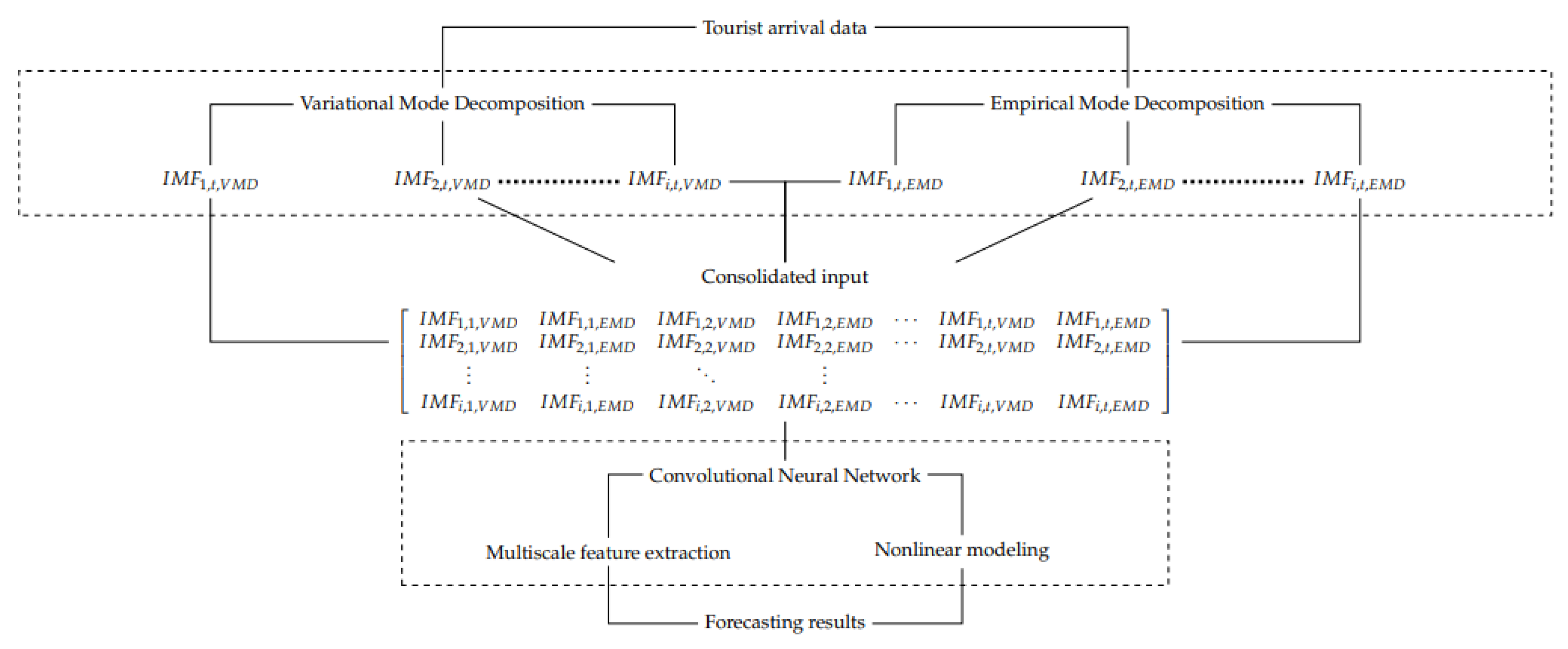
2.3. MD-CNN Forecasting Model

As suggested in numerous empirical studies, there are far too many factors that jointly affect the movement of tourist arrivals. This would result in significant fluctuations in tourist arrival changes with complex and heterogeneous properties. Theoretically, we assume that J influencing factors for tourist arrival y are defined with unique time scale characteristics at time t as in Equation (7):

$$\begin{array}{c}\hfill y_t=\sum _{j=1}^J{c}_{j,t}\end{array}$$

(7)

where $y_t$ is tourist arrival at time t and $c_{j,t}$ is the $j_{th}$ intrinsic modes at time t.

Since the true generating process and multiscale structure are unknown, the multiscale structure for tourist arrival represented by the decomposed data components is determined using m different criteria and algorithm. For example, EMD relies on the stationarity of the decomposed data component to identify the multiscale structure while VMD relies on theoretical guidance to identify multiscale structure. There are estimation biases in both approaches, as in Equation (8):

$$\begin{array}{c}\hfill y_t=\sum _{j=1}^J\sum _{m=1}^M{\widehat{c}}_{j,t,m}+{ϵ}_{m,t}\end{array}$$

(8)

where $y_t$ is the tourist arrival data at t and ${\widehat{c}}_{j,t,m}$ is the $j_{th}$ intrinsic modes at time t using the m mode decomposition model.

The future movement of tourist arrival changes are defined as the function of its estimated J influencing factors over time, using M algorithms under different assumptions and criteria, as in Equation (9)

$$\begin{array}{c}\hfill {\widehat{y}}_{t+1}=f\left(C\right)\end{array}$$

(9)

where $C={\widehat{c}}_{j,t,m},j\in 1,\cdots ,J,t\in 1,\cdots ,T,m\in 1,\cdots ,M$, ${\widehat{y}}_{t+1}$ is the tourist arrival forecast at time $t+1$.

In this paper, we take VMD and EMD as two MD models and CNN as the final estimation model, and propose a new MD-CNN forecasting model. The general structure of the MD-CNN tourist arrival forecasting model is illustrated in Figure 1.

As illustrated in Figure 1, given MD models $m,m\in \{EMD,VMD\}$, the tourist arrival data $y_t$ are decomposed into a series of IMFs accordingly, as in Equation (10).

$$\begin{array}{c}\hfill y_{m,t}=\sum _{j=1}^J{c}_{j,t,m}+r_{m,t},\end{array}$$

(10)

where $y_{m,t}$ is the tourist arrival data using the m mode decomposition model at time t, $c_{j,t,m}$ is the $j_{th}$ intrinsic mode component, and $r_{m,t}$ is the residual component at time t.

IMFs matrices calculated with different MD models $IM{F}_{j,t,m},m=\{EMD,VMD\}$ are combined together to construct the consolidated IMFs matrix as $M_{j,t}$. For example, if EMD and VMD—two major decomposition models in the literature—are used, the consolidated IMF matrix is constructed as in Equation (11):

$$\begin{array}{c}\hfill {\widehat{M}}_{i,t}=\left[\begin{array}{ccccccc}IM{F}_{1,1,VMD}& IM{F}_{1,1,EMD}& IM{F}_{1,2,VMD}& IM{F}_{1,2,EMD}& \cdots & IM{F}_{1,t,VMD}& IM{F}_{1,t,EMD}\\ IM{F}_{2,1,VMD}& IM{F}_{2,1,EMD}& IM{F}_{2,2,VMD}& IM{F}_{2,2,EMD}& \cdots & IM{F}_{2,t,VMD}& IM{F}_{2,t,EMD}\\ ⋮& ⋮& \ddots & ⋮\\ IM{F}_{j,1,VMD}& IM{F}_{j,1,EMD}& IM{F}_{j,2,VMD}& IM{F}_{j,2,EMD}& \cdots & IM{F}_{j,t,VMD}& IM{F}_{j,t,EMD}\end{array}\right]\end{array}$$

(11)

$IM{F}_{j,t,m}$ is the $t_{th}$ intrinsic modes at scale j using multiscale models m.

The Convolutional Neural Network model is used to model the nonlinear map function f between the higher dimensional matrix ${\widehat{M}}_{j,t}$ and the tourist arrival data ${\widehat{y}}_{t+1}$, as in Equation (12).

$$\begin{array}{c}\hfill {\widehat{y}}_{t+1}=f({\widehat{M}}_{j,t})\end{array}$$

(12)

${\widehat{y}}_{t+1}$ is the tourist arrival data at time $t+1$, $f({\widehat{M}}_{j,t})$ is the nonlinear function using CNN.

3. Empirical Results

Data Description and Descriptive Statistics

In our empirical study, Macao is selected as the subject of the empirical analysis to evaluate the forecasting accuracy of different models because it is one of the most active tourist attractions in the world. It receives an active inflow of tourists from around the world and represents an interesting case both for city tourism and international tourism. The dataset for tourist arrival is extensive to reflect the dynamics in the tourism industry so that the modeling accuracy and the generalizations of the MD-CNN model can be evaluated comprehensively in this paper. More importantly, the Macao Government Tourism Office (MGTO) provides data at a daily level while most tourist destinations provide data at a monthly or lower frequency, from the annual statistical report. Therefore, we use the daily tourist arrival data in Macao from five major countries or regions to estimate the model parameters and evaluate the forecasting accuracy of different models. These countries include China, Hong Kong (HK), Indonesia, Philippines, and Singapore. The dataset spans from 1 January 2017 to 13 February 2020 and is preprocessed to remove the anomalies and outliers. The dataset is obtained from the Statistics and Census Service (DSEC), Government of Macao SAR, China. Following the data analysis and machine learning literature, the dataset is divided into three parts with a 49%–21%–30% ratio, which corresponds to the training–validation–test sub-dataset.

The basic descriptive statistics for tourist arrival are reported in

Table 1. Descriptive statistics and statistical tests for tourist arrivals from different countries or regions.

Statistics	${\mathit{Mean}}_{\times {10}^4}$	$\mathit{Standard}{\mathit{Deviation}}_{\times {10}^4}$	Skewness	Kurtosis	$p_{\mathit{JB}}$	$p_{\mathit{BDS}}$
China	6.6678	1.7571	1.4807	7.5316	0.001	0
HK	1.7382	4.7507	1.6218	7.7804	0.001	0
Indonesia	0.0508	0.0290	2.1270	9.0066	0.001	0
Philippines	0.0862	0.0333	1.7717	8.8315	0.001	0
Singapore	0.0374	0.0150	0.6695	3.2716	0.001	0

.

Table 1 shows that tourist arrivals from different countries or regions have a significant level of kurtosis, mostly bigger than 7, except for Singapore. This indicates the prevalence of nonuniform extreme events and significant fluctuations in tourist arrival. Skewness values have positive signs at a non-negligible scale, bigger than 1. Standard deviations also reach the level of significance. The distributions of tourist arrival from different countries or regions do not conform to the normal distribution, indicated by a p-value less than 0.05 for both the Jarque–Bera (JB) test of normality and the BDS test of nonlinear independence. There may exist nonlinear dynamics such as multiscale data features in the tourist arrival changes.

Then, we forecast the MSEs of tourist arrival forecasts in different countries or regions over the time period covered by the validation dataset. The MD-CNN model network structure is Conv1(1,1)-Pool(2,2)-Conv2(1,1)-Pool(2,2)-FC(1) for all countries and regions. Results are reported in

Table 2. Performance of MD-CNN model with different parameters using the model tuning dataset.

Models	MSE${}_{\mathit{China},\times {10}^8}$	MSE${}_{\mathit{HK},\times {10}^7}$	MSE${}_{\mathit{Indonesia},\times {10}^4}$	MSE${}_{\mathit{Philippines},\times {10}^4}$	MSE${}_{\mathit{Singapore},\times {10}^3}$
$MD-CN{N}_{(1,1)}$	1.6773	1.1280	2.3589	7.8064	9.6990
$MD-CN{N}_{(1,2)}$	1.7660	1.1260	2.7853	10.5543	8.3517
$MD-CN{N}_{(2,1)}$	1.7654	1.1214	2.2340	8.2777	8.6854
$MD-CN{N}_{(2,2)}$	1.7365	1.2332	2.3452	9.2343	8.4691

.

$CN{N}_{(k,p)}$ refers to the CNN model with parameter k for the filter size and p for the pooling size. The number of filters is set to 11.

As reported in Table 2, the forecasting accuracy using MD-CNN with different hyperparameters varies. There is no optimal set of hyperparameters for MD-CNN models in all countries or regions. In this paper, we follow the principle of MSE minimization to select the hyperparameters for MD-CNN models with minimal MSE in different countries or regions, respectively. In the end, we chose $MD-CN{N}_{(1,1)}$ in China and Philippines, $MD-CN{N}_{(2,1)}$ for tourist arrivals from HK and Indonesia, and $MD-CN{N}_{(1,2)}$ for tourist arrivals from Singapore, since the parameters are optimized for the tourist arrival of particular countries and regions. This implies that the factors for tourist arrivals from different countries or regions have unique data characteristics and need to be captured within different parameters.

With the optimized parameters, tourist arrivals in different countries or regions are calculated in

Table 3. Model performance using out-of-sample dataset.

Models	MSE${}_{\mathit{China},\times {10}^8}$	MSE${}_{\mathit{HK},\times {10}^7}$	MSE${}_{\mathit{Indonesia},\times {10}^4}$	MSE${}_{\mathit{Philippines},\times {10}^4}$	MSE${}_{\mathit{Singapore},\times {10}^3}$
RW	5.7607	4.4349	8.3045	3.1473	21.5561
ARIMA	2.0019	2.0368	5.4306	1.7129	9.8781
Seasonal ARIMA	1.8434	2.2151	5.8317	1.9324	5.5029
MD-CNN	1.5185	1.6382	2.8709	1.2432	5.0741

; we report the out-of-sample performance comparison using the test data. The model comparison has been conducted between four models, with three benchmark models, i.e., the Random Walk (RW), ARIMA, Seasonal ARIMA models, and our MD-CNN model.

In Table 3, it is clear that the MD-CNN model produces the most accurate forecasts with the smallest MSEs, compared with the performance of the benchmarks RW, ARIMA, and Seasonal ARIMA models.

The superior forecasting performance of the proposed multiscale deep-learning-based model indicates the effectiveness of the incorporation of multiscale data features during the modeling and forecasting process. More specifically, the better performance of the MD-CNN model is attributed to the modeling of multiscale data features during the forecasting process, beyond the linear autocorrelation and seasonal data features captured by the ARIMA and Seasonal ARIMA models. Meanwhile, the better performance of the MD-CNN model compared with the RW model confirms that it is important to consider specific data features such as multiscale and autocorrelation data features in the modeling and forecasting process [36,37,38].

4. Conclusions

In this paper, a new multiscale mode-learning-based (MD-CNN) forecasting model is proposed to predict tourist arrival changes. MD-CNN uses different MD algorithms to model the transient factors. The CNN model is used to aggregate different factors and forecast tourist arrival changes. A comprehensive performance evaluation was conducted using tourist arrival data, which provides empirical evidence for the superior tourist arrival forecasting accuracy of the MD-CNN model.

The success of the introduction of the convolutional neural network model implies that more advanced artificial intelligence models such as deep learning models can contribute to better modeling of tourist arrival change. These models can be designed to target and model specific data features such as multiscale hierarchical structure. Secondly, the results in this paper suggest that the empirical analysis results and the forecasting performance are sensitive to the choice of different multiscale models. The significant model risk may result from the lack of theoretical foundation for the choice of particular multiscale models. Thirdly, the proposed MD-CNN model is constructed as a general multiscale-based forecasting methodology that is flexible enough to be extended to address different modeling issues when it is presented with different tourist destinations data, beyond the Macao tourist arrival data and EMD and VMD models used in this paper.

References

1. Dharmaratne, G.S. Forecasting tourist arrivals in Barbados. Ann. Tour. Res. 1995, 22, 804–818. [Google Scholar] [CrossRef]
2. Hadavandi, E.; Ghanbari, A.; Shahanaghi, K.; Abbasian-Naghneh, S. Tourist arrival forecasting by evolutionary fuzzy systems. Tour. Manag. 2011, 32, 1196–1203. [Google Scholar] [CrossRef]
3. Yang, Y.; Chen, M.H.; Su, C.H.J.; Lin, Y.X. Asymmetric effects of tourist arrivals on the hospitality industry. Int. J. Hosp. Manag. 2020, 84, 102323. [Google Scholar] [CrossRef]
4. Deng, T.; Gan, C.; Du, H.; Hu, Y.; Wang, D. Do high speed rail configurations matter to tourist arrivals? Empirical evidence from China’s prefecture-level cities. Res. Transp. Econom. 2020, 90, 100952. [Google Scholar] [CrossRef]
5. Nguyen, J.; Valadkhani, A. Dynamic responses of tourist arrivals in Australia to currency fluctuations. J. Hosp. Tour. Manag. 2020, 45, 71–78. [Google Scholar] [CrossRef]
6. Huang, L.; Yin, X.; Yang, Y.; Luo, M.; Huang, S.S. Blessing in disguise: The impact of the Wenchuan earthquake on inbound tourist arrivals in Sichuan, China. J. Hosp. Tour. Manag. 2020, 42, 58–66. [Google Scholar] [CrossRef]
7. Demir, E.; Simonyan, S.; Chen, M.H.; Marco Lau, C.K. Asymmetric effects of geopolitical risks on Turkey’s tourist arrivals. J. Hosp. Tour. Manag. 2020, 45, 23–26. [Google Scholar] [CrossRef]
8. Tiwari, A.K.; Das, D.; Dutta, A. Geopolitical risk, economic policy uncertainty and tourist arrivals: Evidence from a developing country. Tour. Manag. 2019, 75, 323–327. [Google Scholar] [CrossRef]
9. Fourie, J.; Santana-Gallego, M. The impact of mega-sport events on tourist arrivals. Tour. Manag. 2011, 32, 1364–1370. [Google Scholar] [CrossRef]
10. Mao, C.K.; Ding, C.G.; Lee, H.Y. Post-SARS tourist arrival recovery patterns: An analysis based on a catastrophe theory. Tour. Manag. 2010, 31, 855–861. [Google Scholar] [CrossRef]
11. Su, Y.W.; Lin, H.L. Analysis of international tourist arrivals worldwide: The role of world heritage sites. Tour. Manag. 2014, 40, 46–58. [Google Scholar] [CrossRef]
12. Yang, C.H.; Lin, H.L.; Han, C.C. Analysis of international tourist arrivals in China: The role of World Heritage Sites. Tour. Manag. 2010, 31, 827–837. [Google Scholar] [CrossRef] [PubMed]
13. Bi, J.-W.; Li, H.; Fan, Z.-P. Tourism demand forecasting with time series imaging: A deep learning model. Ann. Tour. Res. 2021, 90, 103255. [Google Scholar] [CrossRef]
14. Song, H.; Wen, L.; Liu, C. Density tourism demand forecasting revisited. Ann. Tour. Res. 2019, 75, 379–392. [Google Scholar] [CrossRef]
15. Gounopoulos, D.; Petmezas, D.; Santamaria, D. Forecasting Tourist Arrivals in Greece and the Impact of Macroeconomic Shocks from the Countries of Tourists? Origin. Ann. Tour. Res. 2012, 39, 641–666. [Google Scholar] [CrossRef]
16. Song, H.; Li, G. Tourism demand modelling and forecasting—A review of recent research. Tour. Manag. 2008, 29, 203–220. [Google Scholar] [CrossRef]
17. Song, H.; Qiu, R.T.; Park, J. A review of research on tourism demand forecasting: Launching the Annals of Tourism Research Curated Collection on tourism demand forecasting. Ann. Tour. Res. 2019, 75, 338–362. [Google Scholar] [CrossRef]
18. Yang, X.; Pan, B.; Evans, J.A.; Lv, B. Forecasting Chinese tourist volume with search engine data. Tour. Manag. 2015, 46, 386–397. [Google Scholar] [CrossRef]
19. Vergori, A.S. Patterns of seasonality and tourism demand forecasting. Tour. Econ. 2017, 23, 1011–1027. [Google Scholar] [CrossRef]
20. Hassani, H.; Silva, E.S.; Antonakakis, N.; Filis, G.; Gupta, R. Forecasting accuracy evaluation of tourist arrivals. Ann. Tour. Res. 2017, 63, 112–127. [Google Scholar] [CrossRef]
21. Li, S.; Chen, T.; Wang, L.; Ming, C. Effective tourist volume forecasting supported by PCA and improved BPNN using Baidu index. Tour. Manag. 2018, 68, 116–126. [Google Scholar] [CrossRef]
22. Cang, S. A Comparative Analysis of Three Types of Tourism Demand Forecasting Models: Individual, Linear Combination and Non-linear Combination. Int. J. Tour. Res. 2014, 16, 596–607. [Google Scholar] [CrossRef]
23. Long, W.; Lu, Z.; Cui, L. Deep learning-based feature engineering for stock price movement prediction. Knowl. Based Syst. 2019, 164, 163–173. [Google Scholar] [CrossRef]
24. Lahmiri, S.; Bekiros, S. Cryptocurrency forecasting with deep learning chaotic neural networks. Chaos Solitons Fractals 2019, 118, 35–40. [Google Scholar] [CrossRef]
25. Law, R.; Li, G.; Fong, D.K.C.; Han, X. Tourism demand forecasting: A deep learning approach. Ann. Tour. Res. 2019, 75, 410–423. [Google Scholar] [CrossRef]
26. Kulshrestha, A.; Krishnaswamy, V.; Sharma, M. Bayesian BILSTM approach for tourism demand forecasting. Ann. Tour. Res. 2020, 83, 102925. [Google Scholar] [CrossRef]
27. Bi, J.W.; Liu, Y.; Li, H. Daily tourism volume forecasting for tourist attractions. Ann. Tour. Res. 2020, 83, 102923. [Google Scholar] [CrossRef]
28. Chen, J.; Zhu, X.; Zhong, M. Nonlinear effects of financial factors on fluctuations in nonferrous metals prices: A Markov-switching VAR analysis. Resour. Policy 2018, 61, 489–500. [Google Scholar] [CrossRef]
29. Tzirakis, P.; Trigeorgis, G.; Nicolaou, M.A.; Schuller, B.W.; Zafeiriou, S. End-to-End Multimodal Emotion Recognition Using Deep Neural Networks. IEEE J. Sel. Top. Signal Process. 2017, 11, 1301–1309. [Google Scholar] [CrossRef]
30. McCann, M.T.; Jin, K.H.; Unser, M. Convolutional Neural Networks for Inverse Problems in Imaging A review. IEEE Signal Process. Mag. 2017, 34, 85–95. [Google Scholar] [CrossRef]
31. Rawat, W.; Wang, Z. Deep Convolutional Neural Networks for Image Classification: A Comprehensive Review. Neural Comput. 2017, 29, 2352–2449. [Google Scholar] [CrossRef]
32. Lago, J.; Ridder, F.D.; Schutter, B.D. Forecasting spot electricity prices: Deep learning approaches and empirical comparison of traditional algorithms. Appl. Energy 2018, 221, 386–405, Erratum in Appl. Energy 2018, 229, 1286. [Google Scholar] [CrossRef]
33. Peng, B.; Song, H.; Crouch, G.I. A meta-analysis of international tourism demand forecasting and implications for practice. Tour. Manag. 2014, 45, 181–193. [Google Scholar] [CrossRef]
34. Coshall, J.T.; Charlesworth, R. A management orientated approach to combination forecasting of tourism demand. Tour. Manag. 2011, 32, 759–769. [Google Scholar] [CrossRef]
35. Huang, N.E.; Shen, Z.; Long, S.R.; Wu, M.C.; Shih, H.H.; Zheng, Q.; Yen, N.C.; Tung, C.C.; Liu, H.H. The empirical mode decomposition and the Hilbert spectrum for nonlinear and non-stationary time series analysis. Proc. R. Soc. Lond. Ser. A Math. Phys. Eng. Sci. 1998, 454, 903–995. [Google Scholar] [CrossRef]
36. Zhang, C.; Jiang, F.; Wang, S.; Sun, S. A new decomposition ensemble approach for tourism demand forecasting: Evidence from major source countries in Asia-Pacific region. Int. J. Tour. Res. 2021, 23, 832–845. [Google Scholar] [CrossRef]
37. Xing, G.; Sun, S.; Bi, D.; Guo, J.E.; Wang, S. Seasonal and trend forecasting of tourist arrivals: An adaptive multiscale ensemble learning approach. Int. J. Tour. Res. 2022, 24, 425–442. [Google Scholar] [CrossRef]
38. Xie, G.; Qian, Y.; Wang, S. A decomposition-ensemble approach for tourism forecasting. Ann. Tour. Res. 2020, 81, 102891. [Google Scholar] [CrossRef]
39. Wu, Z.; Huang, N.E. Empirical mode decomposition: A noise-assisted data analysis method. Adv. Adapt. Data Anal. 2009, 1, 1–41. [Google Scholar] [CrossRef]
40. Dragomiretskiy, K.; Zosso, D. Variational Mode Decomposition. IEEE Trans. Signal Process. 2014, 62, 531–544. [Google Scholar] [CrossRef]
41. Lecun, Y.; Bottou, L.; Bengio, Y.; Haffner, P. Gradient-based learning applied to document recognition. Proc. IEEE 1998, 86, 2278–2324. [Google Scholar] [CrossRef]
42. van Noord, N.; Postma, E. Learning scale-variant and scale-invariant features for deep image classification. Pattern Recognit. 2017, 61, 583–592. [Google Scholar] [CrossRef]
43. Zou, Y.; Yu, L.; Tso, G.K.; He, K. Risk forecasting in the crude oil market: A multiscale Convolutional Neural Network approach. Phys. A: Stat. Mech. Appl. 2020, 541, 123360. [Google Scholar] [CrossRef]
44. He, K.; Tso, G.K.; Zou, Y.; Liu, J. Crude oil risk forecasting: New evidence from multiscale analysis approach. Energy Econ. 2018, 76, 574–583. [Google Scholar] [CrossRef]
45. He, K.; Zou, Y. Crude oil risk forecasting using mode decomposition based model. Procedia Comput. Sci. 2022, 199, 309–314. [Google Scholar] [CrossRef]
46. Wang, J.; Wang, J. Forecasting stochastic neural network based on financial empirical mode decomposition. Neural Netw. 2017, 90, 8–20. [Google Scholar] [CrossRef]
47. Qiu, X.; Ren, Y.; Suganthan, P.N.; Amaratunga, G.A. Empirical Mode Decomposition based ensemble deep learning for load demand time series forecasting. Appl. Soft Comput. 2017, 54, 246–255. [Google Scholar] [CrossRef]
48. Torres, M.E.; Colominas, M.A.; Schlotthauer, G.; Flandrin, P. A complete ensemble empirical mode decomposition with adaptive noise. In Proceedings of the 2011 IEEE International Conference on Acoustics, Speech and Signal Processing (ICASSP), Prague, Czech Republic, 22–27 May 2011; pp. 4144–4147. [Google Scholar] [CrossRef]
49. Yeh, J.R.; Shieh, J.S.; Huang, N.E. Complementary ensemble empirical mode decomposition: A novel noise enhanced data analysis method. Adv. Adapt. Data Anal. 2010, 2, 135–156. [Google Scholar] [CrossRef]
50. Liu, T.; Luo, Z.; Huang, J.; Yan, S. A Comparative Study of Four Kinds of Adaptive Decomposition Algorithms and Their Applications. Sensors 2018, 18, 2120. [Google Scholar] [CrossRef]
51. Schmidhuber, J. Deep learning in neural networks: An overview. Neural Netw. 2015, 61, 85–117. [Google Scholar] [CrossRef]
52. Hinton, G.E.; Salakhutdinov, R.R. Reducing the dimensionality of data with neural networks. Science 2006, 313, 504. [Google Scholar] [CrossRef] [PubMed]
53. Hinton, G.E.; Osindero, S.; Teh, Y.W. A Fast Learning Algorithm for Deep Belief Nets. Neural Comput. 2014, 18, 1527–1554. [Google Scholar] [CrossRef] [PubMed]
54. Liu, C.; Hou, W.; Liu, D. Foreign Exchange Rates Forecasting with Convolutional Neural Network. Neural Process. Lett. 2017, 46, 1095–1119. [Google Scholar] [CrossRef]
55. Zhao, Z.; Zhang, Y.; Deng, Y.; Zhang, X. ECG authentication system design incorporating a convolutional neural network and generalized S-Transformation. Comput. Biol. Med. 2018, 102, 168–179. [Google Scholar] [CrossRef] [PubMed]
56. Lee, W.Y.; Park, S.M.; Sim, K.B. Optimal hyperparameter tuning of convolutional neural networks based on the parameter-setting-free harmony search algorithm. Optik 2018, 172, 359–367. [Google Scholar] [CrossRef]
Figure 1. Flowchart for the MD-CNN model.
Mathematics 10 02999 g001