Research on Improved BBO Algorithm and Its Application in Optimal Scheduling of Micro-Grid

Abstract

Aiming at the cooperative optimization problem of economy and environmental protection of the traditional microgrid, including micro gas turbine and diesel engine, carbon capture and storage, and a power to gas system which can consume wind and light and deal with carbon dioxide, is introduced, and three optimization scheduling models of the microgrid based on improved BBO algorithm are proposed. Firstly, a micro-grid with a power to gas system is constructed, and an optimal scheduling model is built which takes into account the system operation cost, environmental governance cost and comprehensive economic benefit. Secondly, the ecological expansion operation is introduced, an improved BBO algorithm is explored by improving the mobility model, and its convergence is derived in detail. Finally, the microgrid system energy optimization scheduling is realized based on the improved BBO algorithm. Compared with the scheduling model that only considers the operation cost or pollution gas control cost, the total cost of the comprehensive economic benefit scheduling model is reduced by 15.5% and 5.5%, respectively, which reflects the reasonableness of the scheduling model and the effectiveness of the improved algorithm.

1. Introduction

Since the development and utilization of renewable energy contribute to coordinating economic development and environmental protection, and the power system is put forward with higher requirements by the current industrial production and residential life, distributed power generation technology has attracted the attention of scholars due to its flexibility in power generation [1]. However, due to the uncertainty and randomness of distributed generation, typically represented by wind turbines and photovoltaics, a great challenge for the safe operation of power systems is posed [2]. To minimize this impact, how to reasonably construct an optimal scheduling model for microgrid energy, improve the utilization of clean energy, and enhance the economic efficiency of the system has become an urgent research problem [3,4,5]. Therefore, it is of great practical significance to study the optimal scheduling of microgrid systems.

The reasonable distribution of working time and output power of each distributed power source is the core of the research on the optimal scheduling of microgrids. In general, the current research on the optimal scheduling of microgrids is divided into three categories. Firstly, the optimal scheduling model of the microgrid is discussed. In [6], an operation optimization model has been established in a hybrid energy system including wind power, photovoltaic, gas turbine, and energy storage, so as to reduce the operating cost of the system. In [7], a two-layer real-time scheduling model of the microgrid based on approximate future cost function (AFCF) has been proposed. A random day-ahead scheduling model for wind power storage systems and irrigation systems was proposed in [8], experiments were carried out in agricultural microgrids, and the results showed that it could not only give full play to the advantages of wind power but also smooth the load curve. In [9], a novel optimal scheduling model based on renewable energy (hydrogen) is proposed, which can further reduce dependence on fossil fuels. Secondly, a representative objective function is constructed. In [10], an objective function including cost, outage probability, pollutant emission, and power balance is proposed and solved by an improved two-file multi-objective evolutionary algorithm based on fuzzy decision making (TA-MAEA). The cooperative game theory technology based on particle swarm optimization algorithm was adopted in [11] to establish a multi-objective function model, which comprehensively considered annual profit and energy reliability indicators. Ref. [12] uses the genetic algorithm NSGA-III based on reference points to solve the Pareto solution set of multi-objective functions which comprehensively consider the economy, reliability, and environmental protection of the microgrid. The multi-objective function of balancing economic benefits and environmental costs was proposed in [13] and solved by an improved artificial bee colony algorithm. Finally, various algorithms for solving the optimization model are proposed. An improved meta-heuristic optimization algorithm called the Multidimensional Firefly Algorithm (MDFA) is proposed in [14] to solve day-ahead scheduling optimization problems. In [15], chaos optimization was added to the adaptive annealing particle swarm optimization algorithm to solve the optimal economic scheduling model of the microgrid. Further, an improved swarm approach is proposed in [16] which is applied to the grid-connected optimal scheduling model. Ref. [17] combines the improved Dragonfly Algorithm (MDA) and Whale Optimization Algorithm (WOA) methods to achieve an economical and reliable solution of the optimal scheduling model.

The above studies have contributed to the optimal scheduling of microgrids, whereas the planning of scheduling strategies, objective functions, and constraints for microgrid systems still deviates from the actual situation. In this paper, based on the above research, a residential microgrid with a carbon capture device and e power-to-gas system based on the traditional microgrid is constructed. And three optimal scheduling models with the lowest system operation cost, the lowest environmental management cost, and the comprehensive economic benefits are established. Then, an improved BBO algorithm is adopted to solve the optimal scheduling models. The energy flow and optimization results of the system under each scheduling model are analyzed in-depth to verify the reasonableness of the comprehensive economically optimal scheduling model and the superiority of the improved algorithm.

2. Microgrid System and Optimal Scheduling Models

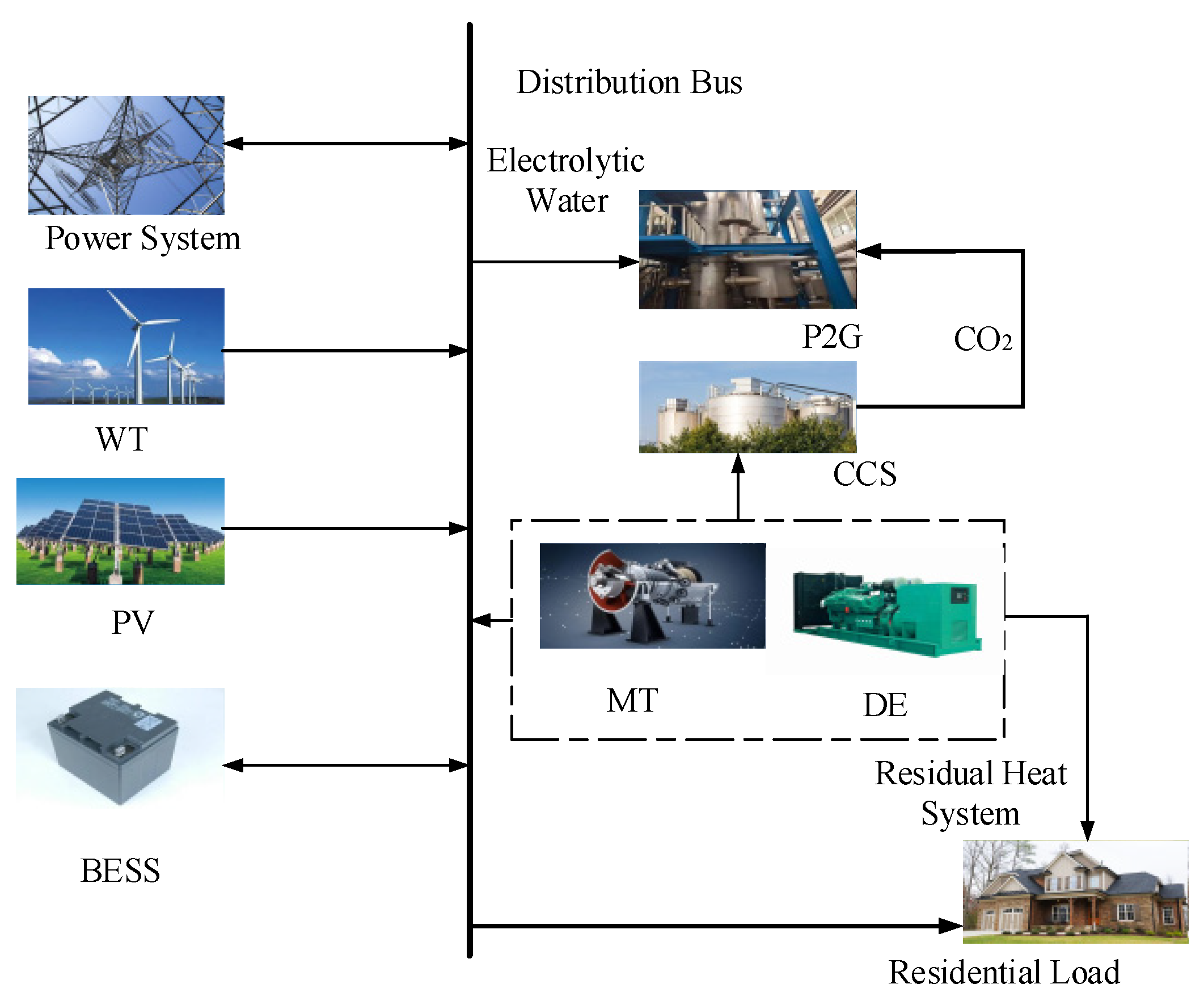
2.1. Microgrids Integrating CCS and P2G

The microgrid integrating carbon capture and storage (CCS) and power to gas (P2G) is shown in Figure 1, which can be subdivided into four parts according to their functions. The energy generation unit consists of distributed generation such as wind turbine (WT), photovoltaic cell (PV), micro turbine (MT), and diesel engine (DE). The energy storage unit mainly contains a battery energy storage system (BESS), carbon capture and storage (CCS), and power to gas (P2G) systems. Load unit refers to an electrical load (Load).

Figure 1. Microgrid system integrating CCS and P2G.

2.2. Optimal Scheduling Models for Microgrid Systems

2.2.1. Scheduling Model Based on the Lowest Cost of System Operation

Considering the economic benefits, the model involves four components of operating costs, and its objective function can be expressed as follows:

$$\min F_1=F_{\mathrm{d}}+F_{\mathrm{c}}+F_{\mathrm{o}}-F_{\mathrm{sell}}$$

(1)

where $F_1$ is the comprehensive operating cost of the microgrid system; $F_{\mathrm{d}}$, $F_{\mathrm{c}}$, $F_{\mathrm{o}}$, and $F_{\mathrm{sell}}$, respectively, represent the energy interaction cost, carbon treatment cost, operating cost of each equipment, and revenue from purchasing and selling electricity of the microgrid and the large power grid.

• The energy interaction cost $F_{\mathrm{d}}$ can be expressed as

  $$F_{\mathrm{d}}={\displaystyle \sum _{t=1}^{24}{P}_{\mathrm{grid}}(t)C_{\mathrm{rgrid}}(t)}$$

  (2)

  where $P_{\mathrm{grid}}(t)$ represents the interactive power between the microgrid and the large power grid; $C_{\mathrm{rgrid}}(t)$ represents the interactive unit price.
• The carbon treatment cost $F_{\mathrm{c}}$ can be calculated with

  $$F_{\mathrm{c}}={\displaystyle \sum _{t=1}^{24}\left(\delta Q_{\mathrm{bu}}(t)+{\delta }_{\mathrm{c}}{P}_{\mathrm{c}}(t)\right)C_{\mathrm{c}}}$$

  (3)

  where $\delta$ represents the power consumption coefficient of CO₂ capture, $\delta =0.7\mathrm{kWh}/{\mathrm{m}}^3$; $Q_{\mathrm{bu}}(t)$ represents the total amount of CO₂ captured; ${\delta }_{\mathrm{c}}$ represents the fixed power consumption factor, ${\delta }_{\mathrm{c}}=0.1$; $P_{\mathrm{c}}(t)$ represents output power; $C_{\mathrm{c}}$ represents the unit price of power output.
• The operating cost $F_{\mathrm{o}}$ is expressed as follows

  $$F_{\mathrm{o}}(t)=\left[\begin{array}{l}{F}_{\mathrm{WT}}(t)+F_{\mathrm{PV}}(t)+F_{\mathrm{MT}}(t)\\ +F_{\mathrm{DE}}(t)+F_{\mathrm{P}2\mathrm{G}}(t)+F_{\mathrm{ech}}(t)\end{array}\right]\times \Delta t$$

  (4)

  where $F_{\mathrm{WT}}(t)$, $F_{\mathrm{PV}}(t)$, $F_{\mathrm{MT}}(t)$, $F_{\mathrm{DE}}(t)$, $F_{\mathrm{P}2\mathrm{G}}(t)$, and $F_{\mathrm{ech}}(t)$ represent the operating costs of WT, PV, MT, DE, P2G, and BESS, respectively.

Specifically, the operating costs of each component are as follows

$$\{\begin{array}{c}{F}_{\mathrm{WT}}(t)=C_{\mathrm{WT}}(t)P_{\mathrm{WT}}(t)\times \Delta t\\ F_{\mathrm{PV}}(t)=C_{\mathrm{PV}}(t)P_{\mathrm{PV}}(t)\times \Delta t\\ \begin{array}{l}{F}_{\mathrm{MT}}(t)=C_{\mathrm{MT}}(t)P_{\mathrm{MT}}(t)\times \Delta t\\ F_{\mathrm{DE}}(t)=C_{\mathrm{DE}}(t)P_{\mathrm{DE}}(t)\times \Delta t\end{array}\\ F_{\mathrm{ech}}(t)=C_{\mathrm{ech}}(t)\mathrm{abs}(P_{\mathrm{ech}}(t))\times \Delta t\\ F_{\mathrm{P}2\mathrm{G}}(t)=C_{\mathrm{P}2\mathrm{G}}(t)P_{\mathrm{P}2\mathrm{G}}(t)\times \Delta t\end{array}$$

(5)

where $C_{\mathrm{WT}}(t)$, $C_{\mathrm{PV}}(t)$, $C_{\mathrm{MT}}(t)$, $C_{\mathrm{DE}}(t)$, $C_{\mathrm{ech}}(t)$, and $C_{\mathrm{P}2\mathrm{G}}(t)$ represent the unit prices of operation and maintenance of each device; $P_{\mathrm{WT}}(t)$, $P_{\mathrm{PV}}(t)$, $P_{\mathrm{MT}}(t)$, $P_{\mathrm{DE}}(t)$, $P_{\mathrm{ech}}(t)$, and $P_{\mathrm{P}2\mathrm{G}}(t)$ represent output power; $\mathrm{abs}$ denotes absolute value.

4.

The revenue from the purchase-sale of electricity is expressed as

$$F_{\mathrm{sell}}(t)=C_{\mathrm{load}}(t)P_{\mathrm{load}}(t)\times \Delta t$$

(6)

where $C_{\mathrm{load}}(t)$ represents the unit price of electricity sold to the large grid; $P_{\mathrm{load}}(t)$ represents the electrical load power.

2.2.2. Scheduling Model Based on Environmental Governance Cost Minimization

Since the cost of environmental pollution only needs to consider the cost of treatment caused by polluting gases generated during the use of MT and DE, it is apparent that the introduction of CCS and P2G is necessary. Table 1 shows the relevant data on pollutant emissions and treatment costs of major equipment. It can be seen from Table 1 that for the same power output (1 kWh), the amount of pollutant gas produced by MT is much lower compared to DE. Thus, the optimal scheduling model based on minimizing the cost of environmental governance can be expressed as [18]:

$$\min F_2=T{\displaystyle \sum _{i=1}^N{C}_i^{\mathrm{emission}}{P}_i}$$

(7)

where $F_2$ represents environmental governance costs; $C_i^{\mathrm{emission}}$ represents polluting gas emission factor, which can be expressed as follows:

$$C_i^{\mathrm{emission}}=C_{{\mathrm{CO}}_2}\times N_i^{{\mathrm{CO}}_2}+C_{{\mathrm{SO}}_2}\times N_i^{{\mathrm{SO}}_2}+C_{{\mathrm{NO}}_{\mathrm{X}}}\times N_i^{{\mathrm{NO}}_{\mathrm{X}}}$$

(8)

where $C_{{\mathrm{CO}}_2}$, $C_{{\mathrm{SO}}_2}$, and $C_{{\mathrm{NO}}_{\mathrm{X}}}$ are the unit price of polluting gas treatment; $N_i^{{\mathrm{CO}}_2}$, $N_i^{{\mathrm{SO}}_2}$, and $N_i^{{\mathrm{NO}}_{\mathrm{X}}}$ represent the emissions of CO₂, SO_2, and NO_X when the micro gas turbine and diesel engine output unit electricity, respectively.

Table 1. Datasheet related to pollutant gas emission and treatment of each equipment.

Polluting Gases	WT (g/(kWh))	PV (g/(kWh))	MT (g/(kWh))	DE (g/(kWh))	Governance Costs (Yuan/kg)
CO2	0	0	729.6	1185	0.025
SO2	0	0	3.36	115.3	6.5
NOX	0	0	1.56	76.74	8.0

2.2.3. Scheduling Model Based on Comprehensive Economic Efficiency Optimization

The two single objectives of minimum system operating cost and minimum environmental governance cost mentioned above conflict with each other. Therefore, the evaluation index of optimal economic efficiency is formulated to take both into account. The expressions are as follows:

$$\min F_3={\phi }_1{F}_1+{\phi }_2{F}_2$$

(9)

$$\{\begin{array}{c}{\phi }_1+{\phi }_2=1\\ 0\le {\phi }_1\le 1,0\le {\phi }_2\le 1\end{array}$$

(10)

where F₃ represents the comprehensive economic benefit considering operating costs and environmental governance costs; ${\phi }_1$ and ${\phi }_2$ denote the weights of two single objectives, respectively.

2.3. Energy Control Strategies for Microgrid System

The grid-connected microgrid with CCS and P2G has been constructed above and three optimal scheduling models are proposed on this basis. The energy control strategy is further presented as shown in Figure 2.

Figure 2. Energy control diagram of the microgrid system.

The operation strategy of the least-cost scheduling model considering system operation is as follows: WT and PV are always at full power while strengthening the output of DE and MT. When the real-time electricity price is high, the BESS needs to remain discharged and the microgrid can peddle the excess power to the larger grid, while when the electricity price is low, the BESS is operated for charging. The microgrid should first purchase power from the grid during this scheduling time to meet the scheduling strategy of the lowest operating cost for this system.

The operation strategy of the scheduling model considering the minimum environmental governance cost is as follows: while WT and PV are at full power, the power generation roles of DE and MT are appropriately weakened, and the CCS device and P2G are ensured to participate in the daily operation of the system, so as to reduce the emission of polluting gases and the environmental governance cost. Regardless of the price of electricity, the main operation is to purchase power from the large power grid, but when the load is large, the power generation of DE and MT must be increased to ensure the stability of the system.

The operation strategy of the optimal scheduling model considering comprehensive economic benefits is: WT and PV are in full power at all times, at the same time, during peak power consumption periods, the working time and output power of DE and MT need to be increased. BESS will contribute the remaining power, and the CCS device and P2G system will cooperate with each other. While during a low power consumption period, the output of DE and MT can be weakened, BESS will store electric energy for assistance at any time, and try to purchase electricity from the large power grid to meet the load demand, so that the system can achieve the optimal goal of comprehensive economic benefits.

3. IBBO Algorithm

The Biogeography-Based Optimization (BBO) algorithm was first proposed by Simon in 2008, which has a simple structure, fewer parameters, and shows good optimality search ability. However, the BBO algorithm still suffers from the problems of limited search range at the beginning of the iteration and the tendency to fall into local optimization at the end of the iteration. An Improved BBO (IBBO) algorithm is proposed to address the aforementioned shortcomings, which introduces a search process and an ecological expansion operation while replacing the linear mobility model with a cosine mobility model, and its flowchart is shown in Figure 3.

Figure 3. IBBO algorithm flow chart.

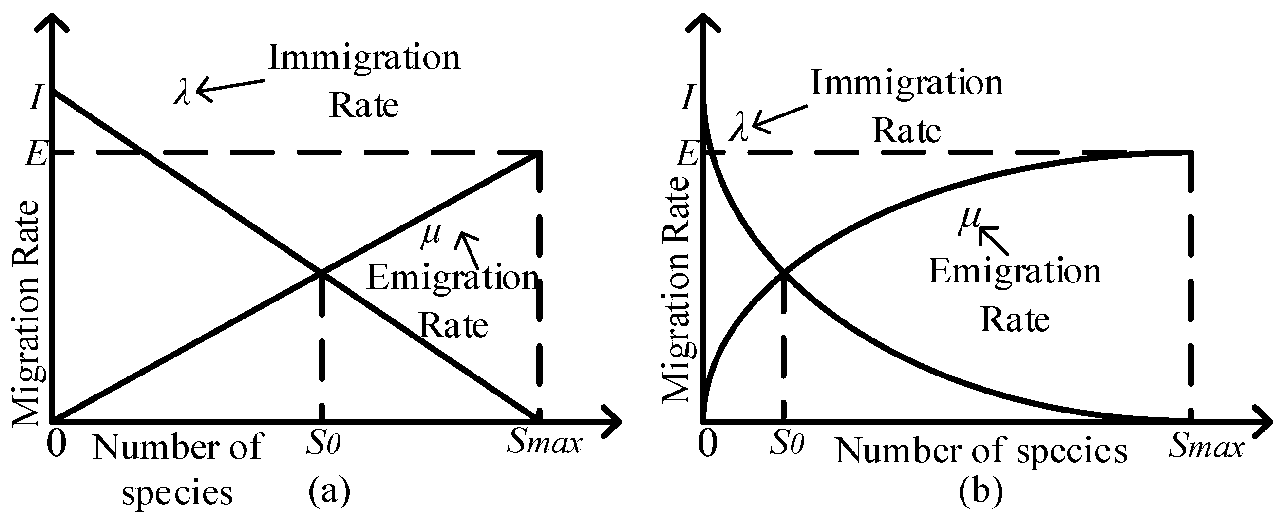
3.1. Cosine Mobility Model

The BBO algorithm is based on a simple linear mobility model, as shown in Figure 4a below, but this model does not work for most optimization problems; thus, IBBO chooses a nonlinear migration model, namely, the cosine mobility model shown in Figure 4b below.

Figure 4. (a) Linear mobility model of species; (b) Nonlinear cosine mobility model of species.

The mathematical expression between the number of species and the migration rate for the cosine migration model is as follows.

$$\{\begin{array}{c}{\lambda }_a=\frac{I}{2}\left(1+\cos \left(\frac{a\pi }{n}\right)\right)\\ {\mu }_a=\frac{E}{2}\left(1-\cos \left(\frac{a\pi }{n}\right)\right)\end{array}$$

(11)

where ${\lambda }_a$ and ${\mu }_a$ represent the immigration and emigration rates for a site with species number $a$; $I$ and $E$ represent the maximum value of $\lambda$ and $\mu$; $a$ and $n$ indicate the current number of species and the upper limit of the number of species that can be carried.

3.2. Search Process

The BBO algorithm obtains the habitat HSI by initializing the data, followed by sorting them from largest to smallest and implementing an elitism strategy, and then performing the migration operation. Once the optimal solution is near the constraint boundary, it will consume some arithmetic power and increase the computational complexity of the algorithm. Therefore, the improved algorithm sets up a search process before the biological migration operation, in other words, it searches for new habitats based on the HSI values of the previous generation of habitats, which has the advantage of enhancing the diversity of the initialized population and improving the search breadth of the algorithm The relationship between the number of new habitats and the HSI of the original habitat is as follows.

$$I_a=\{\begin{array}{cc}{I}_{\min }+\frac{f_a-f_{\min }}{f_{\min }-f_{\max }}(I_{\max }-I_{\min }),& f_{\min }\ne f_{\max }\\ I_{\max },& f_{\min }=f_{\max }\end{array}$$

(12)

where $f_a$ represents the HSI of the habitat when the number of species is $a$; $f_{\max }$ and $f_{\min }$ represent the maximum and minimum values, respectively; $I_a$ indicates the number of new habitats available for search by the species in the habitat; $I_{\max }$ and $I_{\min }$ represent the upper and lower bounds of the number of new habitats searched during each iteration, respectively.

3.3. Ecological Expansion Operation

The probability of ecological expansion of species to more distant habitats decreases in a nonlinear form, so the law of ecological expansion of the IBBO order also satisfies a normal distribution. In other words, the results of the current iteration can expand on new habitats around the results of the previous iteration in a normally distributed form, and the standard deviation of the expansion range of each iteration is as follows:

$$\{\begin{array}{c}{\pi }_{\mathrm{index}}={\pi }_{\mathrm{final}}+{\left(\frac{G_{\max }-G_{\mathrm{index}}}{G_{\max }}\right)}^n({\pi }_{\mathrm{initial}}-{\pi }_{\mathrm{final}})\\ {\pi }_{\mathrm{initial}}>{\pi }_{\mathrm{final}}\end{array}$$

(13)

where ${\pi }_{\mathrm{index}}$ is the standard deviation of the current iteration; ${\pi }_{\mathrm{initial}}$ and ${\pi }_{\mathrm{final}}$ denote the standard deviation of the first iteration and the last iteration, respectively; and ${\pi }_{\mathrm{initial}}>{\pi }_{\mathrm{final}}$; therefore, the algorithm can obtain a broader search range in the first iteration, while facilitating deep data mining in the later stage; $G_{\max }$ is the maximum number of iterations; $n$ is the parameter.

The migration mechanism of the conventional BBO algorithm exhibits inter-habitat SIV transfer through roulette wheel operations; whereas the migration operation is added by IBBO with a discriminatory mechanism to minimize the probability of migration of poor quality SIV vectors to high-quality SIV vectors: If the condition is satisfied, migration of high-quality SIV vectors to poor quality SIV vectors is allowed, otherwise, the ecological expansion operation is performed. The addition of the eco-expansion operation further enhances the ability of inferior solution vector improvement, and the overall performance of the algorithm is drastically improved.

3.4. Convergence Analysis

The following two preconditions can be given according to the BBO model. One is that the next solution set will be generated regardless of whether the current solution set is replaced or not, and the other is that the relevant elements of the current solution set can be contained by the next solution set. Based on these two assumptions, the transition of a habitat from one state to another in the IBBO algorithm can be expressed as follows:

$${\mathit{H}}^{i,j}\to {\mathit{H}}^{k,l}$$

(14)

where ${\mathit{H}}^{i,j}\left(i=1,2,\cdots ,n,j=1,2,\cdots ,\left|H_S^i\right|\right)$ is the $j$th state of the solution set $H_S^k$; $p_{ij,kl}$ represents the probability of conversion of the equation; $p_{ij,k}$ denotes the probability of change from ${\mathit{H}}^{i,j}$ to $H_S^k$; $p_{i\to k}$ denotes the transition probability from $H_S^i$ to $H_S^k$.Then, the following relation is established:

$$\{\begin{array}{c}{p}_{ij,k}={\displaystyle \sum _{l=1}^{\left|H_S^i\right|}{p}_{ij,kl}},{\displaystyle \sum _{k=1}^N{p}_{ij,k}=1},\\ p_{i,k}\ge p_{ij,k}\Rightarrow {\displaystyle \sum _{k=1}^N{p}_{i\to k}\ge {\displaystyle \sum _{k=1}^N{p}_{ij,k}=1},}\\ 0\le {\displaystyle \sum _{k=1}^N{p}_{i\to k}\le 1},{\displaystyle \sum _{k=1}^N{p}_{i\to k}=1}\end{array}$$

(15)

In conjunction with the above, the following inference is further given: If $\forall {\mathit{H}}^{i,j}\in H_S^i$, it means that $\forall k>i,p_{i\to j}=0$ and $\exists k<i,p_{i\to j}>0$, where $H_S^i$ represents the state of a habitat suitability index $(H_{s,t})$ at time $t$. Since the state of the solution set obtained from the current iteration of IBBO is only related to the previous iteration and the best solution is obtained for each iteration, this indicates that the state $i$ is the best state reached by the habitat so far, so the current state is as follows:

$$F(H_{s,t+1})\le F(H_{s,t})$$

(16)

where $F(H_{s,t})$ is the optimal solution of the test function at time $t$.

In addition, the above formula is modified as follows:

$$\forall k>i,p(H_{s,t})\Rightarrow p(H_{s,t+1})=0$$

(17)

Therefore, the following conclusions can be drawn:

$$\{\begin{array}{l}\forall k>i,p_{i\to j}=0\\ \exists k<i,p_{i\to j}>0\end{array}$$

(18)

The following relation can be obtained combined with the relevant definition and properties of Markov chains. Define $\mathit{C}$ as a random m-order matrix, then a n-order matrix ${\mathit{P}}^{\prime }$ can be obtained by $\mathit{C}$ through a series of transformations. Define ${\mathit{P}}^{\prime }$ as a regulatable random matrix with the following specific characteristics:

$$\{\begin{array}{l}{\mathit{P}}^{\prime }=\left[\begin{array}{cc}\mathit{C}& \mathbf{0}\\ \mathit{R}& \mathit{T}\end{array}\right]\Rightarrow {({\mathit{P}}^{\prime })}^{\infty }=\underset{k\to \infty }{\lim }{({\mathit{P}}^{\prime })}^k\\ =\underset{k\to \infty }{\lim }\left[\begin{array}{cc}{\mathit{C}}^k& \mathbf{0}\\ {\displaystyle \sum _{i=1}^{k-1}{\mathit{T}}^i\mathit{R}{\mathit{C}}^{k-i}}& {\mathit{T}}^k\end{array}\right]=\left[\begin{array}{cc}{\mathit{C}}^{\infty }& \mathbf{0}\\ {\mathit{R}}^{\infty }& \mathbf{0}\end{array}\right]\end{array}$$

(19)

where $\mathit{R}\ne \mathbf{0}$; $\mathit{T}\ne \mathbf{0}$.

In addition, the relevant constraints on the regulatable random matrix ${\mathit{P}}^{\prime }$ are given by

$$\{\begin{array}{c}{({\mathit{P}}^{\prime })}^{\infty }={\left[p_{i\to j}\right]}_{n\times n},\\ p_{i\to j}>0,1\le i\le n,1\le j\le m,\\ p_{i\to j}=0,1\le i\le n,m<j\le n\end{array}$$

(20)

Discussing the global convergence of IBBO according to Equations (18) and (20), $H_s^i(i=1,2,\cdots ,n)$ can be considered as a state on a finite Markov chain at one point, and the following equation is given:

$${\mathit{P}}^{\prime }=\left[\begin{array}{cccc}{p}_{1\to 1}& 0& \cdots & 0\\ p_{2\to 1}& p_{2\to 2}& \cdots & 0\\ ⋮& ⋮& \ddots & ⋮\\ p_{n\to 1}& p_{n\to 2}& \cdots & p_{n\to n}\end{array}\right]=\left[\begin{array}{cc}\mathit{C}& \mathbf{0}\\ \mathit{R}& \mathit{T}\end{array}\right]$$

(21)

Details on the components of the matrix are manifested as

$$\{\begin{array}{c}\mathit{C}=(p_{1\to 1})=(1)\ne \mathbf{0}\\ \mathit{T}=\left[\begin{array}{ccc}{p}_{2\to 2}& \cdots & 0\\ ⋮& \ddots & ⋮\\ p_{n\to 2}& \cdots & p_{n\to n}\end{array}\right]\ne \mathbf{0}\\ p_{2\to 1}>0\Rightarrow \mathit{R}={(p_{2\to 1},\cdots ,p_{n\to 1})}^{\mathrm{T}}\ne \mathbf{0}\end{array}$$

(22)

Therefore, ${\mathit{P}}^{\prime }$ is a statutable random matrix and approaches infinity with the number of iterations, which means that

$${({\mathit{P}}^{\prime })}^{\infty }=\underset{k\to \infty }{\lim }\left[\begin{array}{cc}{\mathit{C}}^k& \mathbf{0}\\ {\displaystyle \sum _{i=1}^{k-1}{\mathit{T}}^i\mathit{R}{\mathit{C}}^{k-i}}& {\mathit{T}}^k\end{array}\right]=\left[\begin{array}{cc}{\mathit{C}}^{\infty }& \mathbf{0}\\ {\mathit{R}}^{\infty }& \mathbf{0}\end{array}\right]$$

(23)

where ${\mathit{C}}^{\infty }=\mathit{C}=(1)$; ${\mathit{T}}^{\infty }=\mathbf{0}$.

It is considered that in the Markov transformation matrix (${\mathit{P}}^{\prime }$), if the occurrence probability of each row element is added, the final result is 1, as ${\mathit{R}}^{\infty }={(1,1,\cdots ,1)}^{\mathrm{T}}$; hence, the inference is given by

$${\mathit{P}}^{\prime }=\left[\begin{array}{cc}{\mathit{C}}^{\infty }& \mathbf{0}\\ {\mathit{R}}^{\infty }& \mathbf{0}\end{array}\right]=\left[\begin{array}{cccc}1& 0& \cdots & 0\\ 1& 0& \cdots & 0\\ ⋮& ⋮& \ddots & ⋮\\ 1& 0& \cdots & 0\end{array}\right]$$

(24)

Research of the above proof process suggests that when $k\to \infty$, ${{\displaystyle p}}_{i\to 1}(i=1,2,\cdots ,n)=1$, which implies the reasonableness and correctness of the equation shown as

$$\underset{t\to \infty }{\lim }\{F(H_{i,t})\to F(H^{\ast })\}=1(i=1,2,\cdots ,n)$$

(25)

it can be evidenced that regardless of the initial situation of the solution set of iterations, as the number of iterations increases, the probability of convergence to the global optimal solution is one. As above, the convergence of IBBO algorithm has been proved.

4. Simulations and Discussion

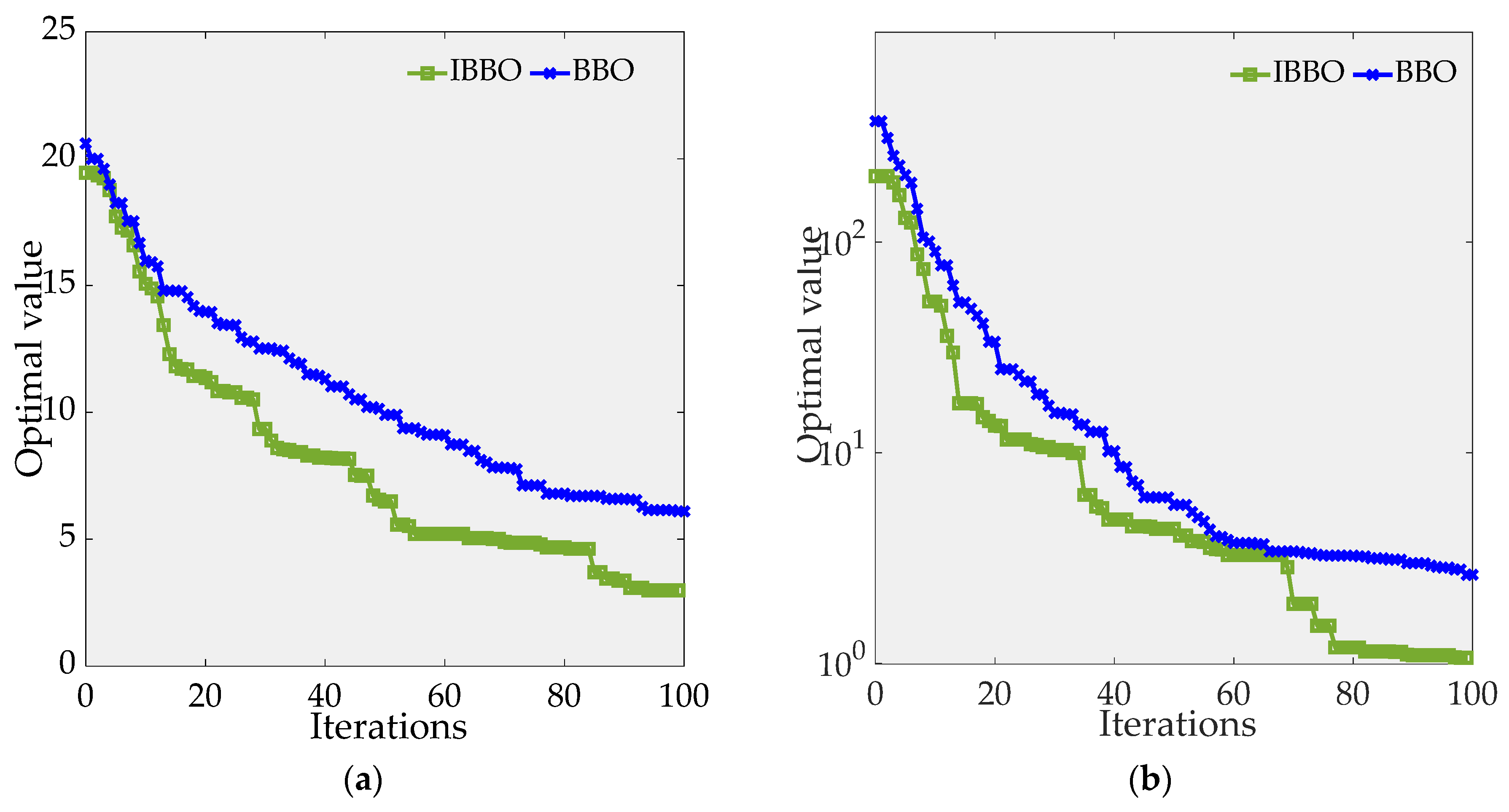
4.1. IBBO Performance Analysis

In order to test the effectiveness of the improved algorithm, an experimental comparison is performed with the traditional BBO algorithm based on six benchmark functions. Six typical optimization performance test functions in CEC2014 are selected, and the optimal solutions of the functions are located at the origin. The description of their properties is specified in Table 2.

Table 2. Benchmark functions characteristic description.

Function	Expression	Space	Dimension
$f_1$ (Ackley)	$\begin{array}{ll}{f}_1\left(x\right)& =-20\exp \left(-0.2\sqrt{\frac{{\displaystyle {\sum }_{i=1}^n{x}_i^2}}{n}}\right)-\\ & \exp \left(\frac{{\displaystyle {\sum }_{i=1}^n\cos \left(2\pi x_i\right)}}{n}\right)+20+e\end{array}$	$-32\le x_i\le 32$	30
$f_2$ (Griewank)	$f_2\left(x\right)={\displaystyle \sum _{i=1}^n\frac{x_i^2}{4000}}-{\displaystyle \prod _{i=1}^n\left(\cos \left(\frac{x_i}{\sqrt{i}}\right)\right)}+1$	$-600\le x_i\le 600$	30
$f_3$ (Rastrigin)	$f_3\left(x\right)=10n+{\displaystyle \sum _{i=1}^n\left(x_i{}^2-10\cos \left(2\pi x_i\right)\right)}$	$-10\le x_i\le 10$	30
$f_4$ (Rosenbrock)	$f_4\left(x\right)={\displaystyle \sum _{i=1}^{n-1}\left[100{\left(x_{i+1}-x_i^2\right)}^2+{\left(1-x_i\right)}^2\right]}$	$-2\le x_i\le 2$	30
$f_5$ (Schewefel2.21)	$f_5\left(x\right)=\max \left\{\left|{{\displaystyle x}}_i\right|,1\le i\le D\right\}$	$-5.12\le x_i\le 5.12$	30
$f_6$ (Step)	$f_6\left(x\right)={\displaystyle \sum _{i=1}^n{\left(\left[x_i+0.5\right]\right)}^2}$	$-100\le x_i\le 100$	30

In order to ensure the reliability of the experimental data, all common parameters of BBO and IBBO are set the same in this paper. The specific settings are as follows: population size is $N=100$, feature dimension is $D=30$, global migration rate is $P_{\mathrm{mod}}=1$, maximum in-migration rate $I$ and maximum out-migration rate $E$ are 1, and maximum mutation rate is $M_{\max }=0.05$; the Gaussian mutation rate is also set as $0.05$, the elite retains individuals is $Keep=2$, and the maximum number of iterations is $G_{\max }=100$.

For the sake of more comprehensive evaluation of the optimization performance of the algorithms and to avoid the influence of experimental chance, 50 Monte Carlo experiments are used as the benchmark, and the metrics of Average Value (Avg), Optimal Value (OV), Standard Deviation (Std), and Mode are used to evaluate algorithms. The experimental data are shown in Table 3, and the best-performing data of each indicator for each function are in bold.

Table 3. Experimental data based on six benchmark functions.

Function	Algorithm	Avg	OV	Std	Mode
$f_1$	BBO	1.07 × 101	6.12 × 100	3.88 × 100	6.75 × 100
	IBBO	8.04 × 100	2.97 × 100	4.51 × 100	5.21 × 100
$f_2$	BBO	3.46 × 101	2.63 × 100	7.38 × 101	3.94 × 100
	IBBO	2.05 × 101	1.06 × 100	4.59 × 101	3.26 × 100
$f_3$	BBO	4.42 × 101	1.49 × 101	5.88 × 101	1.77 × 101
	IBBO	2.51 × 101	0	5.03 × 101	0
$f_4$	BBO	2.70 × 102	9.64 × 101	5.85 × 102	1.12 × 102
	IBBO	1.64 × 102	2.19 × 101	4.20 × 102	2.19 × 101
$f_5$	BBO	1.03 × 101	5.83 × 10−1	2.34 × 101	8.83 × 10−1
	IBBO	6.91 × 100	0	1.47 × 101	0
$f_6$	BBO	3.48 × 103	1.55 × 102	7.12 × 103	1.55 × 102
	IBBO	2.26 × 103	7.63 × 101	4.84 × 103	7.57 × 102

It is evident from Table 3 that in terms of Avg, OV, and Mode, the data obtained by the IBBO algorithm firmly take the lead, especially for the functions $f_3$ and $f_5$; the IBBO algorithm approximates the optimal solution of the test function, which fully reflects the crushing advantage over the traditional algorithm. In the case of the same parameters, the IBBO algorithm mostly converges to smaller values compared to the classical algorithm, indicating a better optimization effect.

Moreover, to further evaluate the algorithm’s optimization-seeking ability, the iteration curves of the two algorithms on the six benchmark functions can be visualized by Figure 5a–f, where(a)–(f) represent the convergence curves of $f_1$–$f_6$, respectively.

Figure 5. Iterative graphs of two algorithms based on six benchmark functions. (a) $f_1$ (Ackley); (b) $f_2$ (Griewank); (c) $f_3$ (Rastrigin); (d) $f_4$ (Rosenbrock); (e) $f_5$ (Schewefel2.21); (f) $f_6$ (Step).

From Figure 5, it can be observed that the optimal values of each function in the initial stage of the iteration differ significantly, and the optimal value of the function $f_1$ obtained by the IBBO algorithm is 18, while the value obtained by BBO exceeds 20. It is more obvious for the function $f_6$, where the initial solution of IBBO is 2.4 × 10⁴, which is much better than the other algorithm. For the function $f_3$–$f_5$, the performance of each algorithm in the initial stage is similar. It can be seen that the IBBO algorithm can enter the working state more quickly at the beginning of the iteration, which laterally reflects that adding the search process before the migration operation can enhance the population diversity, and indicates the rationality of this improvement strategy. From the perspective of convergence speed and optimization accuracy, the convergence curve effect of IBBO is much better than that of BBO for all tested functions, indicating that the introduction of eco-expansion operation has achieved good results. Moreover, combined with the images, it is visible that IBBO shows a better evolutionary curve from the beginning of the iteration to the final end. Compared with the BBO algorithm, IBBO shows a stronger search capability in the late iteration, while BBO is caught in a local search for superiority. It can be demonstrated that the overall performance of the IBBO algorithm is better.

Three scheduling models for microgrid systems have been proposed in the previous section, and the technical parameters of each distributed power supply associated with them are shown in Table 4.

Table 4. Technical parameters of each distributed power supply.

Power Supply	Output Power (kW)	Rated Power (kW)	Coefficient	Maintenance Costs (Yuan/kWh)	Service Life (Year)
WT	0–480	500	0.2098	0.12	10
PV	0–480	500	0.0092	0.08	20
MT	0–1000	1000	0.0473	0.06	15
DE	0–800	800	0.0836	0.04	15

Other parameters are set as follows: The hourly power interaction with the grid is $\pm 150\mathrm{kW}$. The storage device is a battery with a capacity of $600\mathrm{kW}$, whose charging and discharging power is $80\mathrm{kW}$, charging and discharging efficiency is $90\%$, charging and discharging cost is $0.01\mathrm{Yuan}/\mathrm{kWh}$, the state of charge is $50\mathrm{kWh}–550\mathrm{kWh}$, and its maintenance cost is $0.01\mathrm{Yuan}/\mathrm{kWh}$; the operating efficiency of P2G is set to $60\%$, and the capacity is $600\mathrm{kWh}$.

Then, the multi-objective function of the optimal comprehensive economic benefits of the microgrid will be explored based on the IBBO algorithm, and its investigation process is shown in Figure 6.

Figure 6. Solution flow of micro-grid optimal scheduling model.

The detailed steps of the IBBO algorithm for solving the three optimal scheduling models are divided into the following.

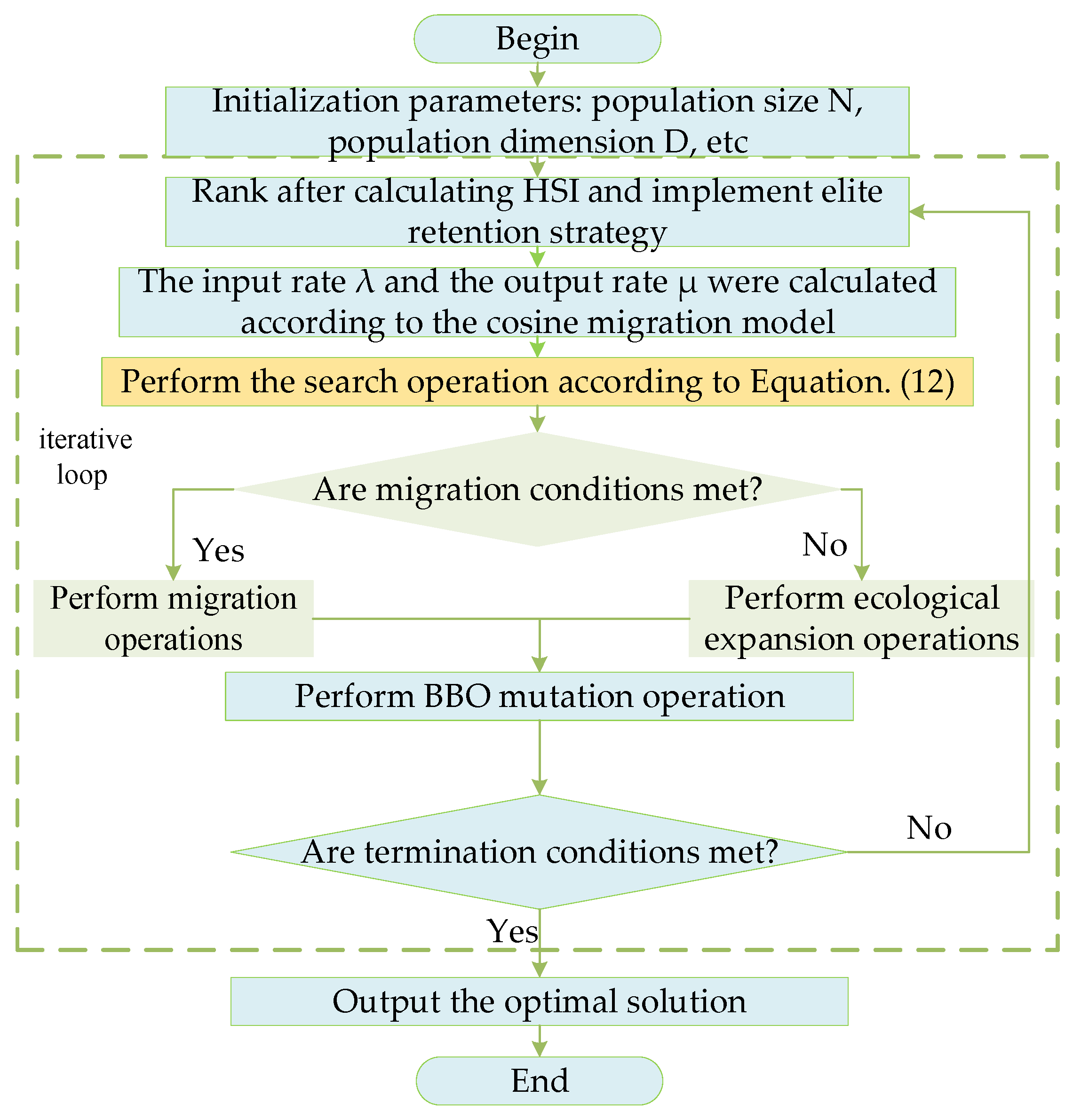
• Initialization parameters

For the multi-objective function, set the parameters as follows: the population size is set to $N=50$, the maximum immigration rate $I$ and the maximum emigration rate $E$ are both $1$; further, the values of the maximum mutation rate and Gaussian mutation rate are 0.05, respectively; the elite preservation individuals are assumed as $Keep=2$; the maximum iteration number is defined as $G_{\max }=100$; The weights of the objective function are respectively defined as ${\phi }_1=0.6$, ${\phi }_2=0.4$.

2.

Migration

Firstly, the suitability component of the habitat is randomly initialized, which means that the minimum system operation cost and the minimum environmental management cost are calculated according to Equations (1) and (7), respectively. Then, the objective function value of the optimal comprehensive economic efficiency is derived according to Equation (9), while the feasible solutions are arranged in the order from largest to smallest. Finally, a hybrid migration operation is performed with the current optimal solution as the evolutionary direction to update the objective function values.

3.

Mutation

The new solutions of objective function values can be formed by mixing variants to improve the diversity of solution sets.

4.

Elite preservation operation

At each iteration, the optimal value of the objective function and the output power of each corresponding equipment component are kept as the elite generation 2, on which the output power of each distributed power source of the microgrid is updated, and the next iteration is carried out until the instruction to terminate the iteration is received.

4.2. Optimal Scheduling Considering System Operating Costs

When only the single objective function with the lowest operating cost of the microgrid system is considered, the output of each installation needs to be considered in terms of the generation cost of the distributed power sources. Compared with conventional DE and MT, CCS and P2G operate at a higher cost. Therefore, their output is not considered in this scenario, and only the optimized dispatch of DE, MT, WT, PV, and BESS is considered, as demonstrated in Figure 7.

Figure 7. Energy scheduling considering system operation cost.

As can be seen from Figure 7, the scenario is dominated by DE, which has lower generation costs but is environmentally unfriendly, then followed by MT and WT. For the sake of reducing the operation and maintenance costs, power purchase from the larger grid is only considered when the total system power output cannot meet the load demand. When the load demand is low during the 0:00–5:00 phase, the DE only needs to maintain a certain output power. Due to the low electricity prices at this time, the battery goes into a charging state. At 6:00 sunrise, PV starts to work with solar energy, and MT gradually increases the power output. Meanwhile, the stored power of the battery has reached the upper limit and is always ready to enter the discharge state. At this moment, the whole system has no power supply pressure, so we can consider selling the excess power to the large grid. During 10:00–12:00, residents start their normal production and life and the demand for electricity increases significantly, and the peak demand is reached at 12:00. At this stage, DE is approaching full generation, and WT, PV, BESS, and MT also assist in generating power to increase the system output. The load demand dropped significantly between 12:00 and 16:00. The MT and DE, which were previously operating at high speed, reduce their output power to improve the service life of the equipment and reduce maintenance costs. At the same time, there is not much power left in the battery, so its output power drops rapidly. When the evening peak of electricity consumption arrives at 16:00–20:00, all the distributed power sources work together to produce power. Even though the electricity price is higher at this time, the microgrid system must purchase power from the larger grid to ensure a safe and smooth operating environment. After 20:00, the load demand drops significantly, and DE and MT cooperate to ensure the stable power output, while the battery quickly enters the charging state to replenish the power.

4.3. Optimal Scheduling Considering Environmental Governance Costs

When only the objective function of minimizing the environmental governance costs of the microgrid system is considered, it is necessary to coordinate the output of the main equipment in terms of both the source and the management of polluting gases. The following Figure 8 demonstrates where only environmental management costs are considered while system operating costs are not. Figure 7 depicts the following phenomenon. As energy conversion units for treating polluting gases, CCS and P2G will not generate electricity, but they will participate in the process of treating polluting gases and consume a certain amount of electricity. The power consumed during processing is positively correlated with the load demand, and the operating time of the P2G system increases accordingly.

Figure 8. Energy scheduling considering environmental treatment cost.

The load value gradually increases from 0:00 to 7:00. At this time, MT, which is more efficient in generating electricity and produces less polluting gases, is the first to produce power. Due to the low price of electricity at this time, the excess electricity is stored, thus avoiding a certain moment when the system is forced to generate electricity due to insufficient storage and pollutes the environment, which means that the goal of minimizing the cost of environmental management is achieved. After 8:00, the electricity price is on the rise and the storage capacity of the battery has reached the upper limit, so the charging operation can no longer be performed. Therefore, the excess electricity can be used for the P2G system to guarantee its stable operation for better treatment of polluting gases. After 9:00, the load demand rises sharply and gradually increases to the peak. The battery soon entered the discharge state, and the MT continued to generate power at full capacity, and the PV power generation also reached its peak at this moment. In the face of the large power supply pressure, even the DE unit, which is not friendly to the environment, immediately switched to a high-speed operation mode to ensure a large amount of power output. During 12:00–16:00, load demand decreases, MT still plays a major role, while DE unit and battery output power are significantly reduced. During 16:00–20:00, when the remaining capacity of the battery is insufficient, the DE unit takes on more output, which works together with WT and MT to ensure the continuous supply of electricity. After 20:00, as the load demand gradually decreases, the power consumed by P2G also decreases. The MT power output is dominated and the WT assists, while the BESS shifts to charging.

4.4. Optimal Scheduling Considering Comprehensive Economic Benefits

The optimized microgrid system energy dispatch is obtained based on the IBBO algorithm in the optimal scheduling model considering the optimal system economic efficiency, as shown in Figure 9.

Figure 9. Energy scheduling considering comprehensive economic benefits.

Between 0:00 and 3:00, the load demand increases within a certain range. Due to the low price of electricity, the system mainly purchases electricity from the larger grid, thus balancing the cost of power generation with the cost of environmental management, as well as WT, DE, and MT also maintaining the power output of varying sizes. The overall output power of the system is sufficient to meet the load demand, so BESS stores the surplus power. From 3:00 to 8:00, there will be an overall increase in the demand for electrical energy to meet the production and living needs of residents. At 4:00, the storage capacity of BESS reaches its upper limit. As the electricity price starts to rise, it can be observed that the system significantly reduces the power purchase from the larger grid and the DE and MT also increase the output power to varying degrees. From 8:00–12:00, the load increases significantly. The DE and MT are operating at roughly 500 kWh, which not only ensures the stable output of electric energy but also reduces the emission of polluting gases to the greatest extent. For the consideration of system power generation cost, BESS started to discharge and work together with other distributed power sources to maintain the safe and smooth operation of the whole system. From 12:00–16:00, the load drops. DE and MT basically maintain a power output of 500 kWh, while the discharge of BESS gradually decreases. From 16:00–20:00, when electricity prices are higher, part of the electricity is sold by the system to the larger grid for profit, thus reducing operating costs. During 20:00–24:00, MT can contribute a certain amount of electricity, and considering the low price of electricity at this time, it is a reasonable choice to purchase electricity from the large grid. In addition, DE and MT rapidly reduce the output power to reduce the cost of environmental governance, and BESS enters the charging state.

In general, in this scheduling model, the microgrid system purchases power from the large grid most of the time to supply the load demand. During the period when the load demand is high or the electricity price is high, the BESS is discharging and the MT and DE increase the power generation accordingly. In addition, the MT and DE do not operate at full power but keep their output power at about 500 kWh. Conversely, when the load demand is low or the electricity price is low, the BESS starts charging and the MT and DE output power is relatively lower.

In this paper, the microgrid system is optimally scheduled for the three objectives of operating cost, environmental management cost, and comprehensive economic benefits, and the comparison of the optimization results is shown in the following Table 5.

Table 5. Comparison of optimization results of three scheduling models.

Objective Functions	System Operating Cost (Yuan)	Environmental Governance Cost (Yuan)	Total Cost (Yuan)
Lowest system operating cost	1432.1	1387.3	2819.4
Lowest environmental governance cost	1899.7	620.4	2520.1
Optimal comprehensive economic benefits	1747.9	632.9	2380.8

From the optimization results in Table 5, it can be seen that if only the system operation cost is considered, the DE with good power generation effect but not friendly to the environment will undertake more; therefore, the environmental management cost is larger. If only the environmental management cost is considered, DE and MT will work fewer hours to some extent. To meet the load demand, the system will inevitably increase the electricity purchase from the larger grid, leading to an increase in system cost. Compared with these two scheduling models mentioned previously, the total cost considering the multi-objective scheduling model is 2380.8 Yuan, which is better than 2819.4 Yuan and 2520.1 Yuan under the other two scheduling models, with a reduction of 15.5% and 5.5%, respectively. The results demonstrate that it makes more reasonable scheduling of the working time and output power of each distributed power source, which laterally reflects the effectiveness and feasibility of the optimal scheduling model.

5. Conclusions

A home-based microgrid system with a carbon capture device and P2G is constructed in this paper. Considering the economy and environmental protection of this microgrid, the corresponding dispatching strategy is formulated. Moreover, the single-objective optimal scheduling model with the lowest operating cost and the lowest environmental governance cost is proposed respectively and the multi-objective optimal scheduling model with optimal comprehensive economic efficiency is also proposed. At the same time, the IBBO algorithm was studied based on improving the migration rate model and increasing the search process and ecological expansion operation, which showed that the overall performance of the IBBO algorithm was better. Finally, an investigation of the optimal scheduling of energy in microgrids is carried out based on the improved BBO algorithm, and the flow of energy after optimal scheduling is analyzed in detail. The optimization results demonstrate the superiority of the multi-objective optimal scheduling model considering comprehensive economic benefits.

References

1. Liu, C.; Wang, H.; Li, T.; Jin, X.; Li, Z. Study on influence of distributed new energy generation on distribution network voltage. Renew. Energy Resour. 2019, 37, 1465–1471. [Google Scholar]
2. Song, X.; Han, L.; Ju, H.; Chen, W.; Peng, Z.; Huang, F. A review on development practice of smart grid technology in China. Electr. Power Constr. 2016, 37, 1–11. [Google Scholar]
3. Guo, P.; Liu, W.; Dan, Y.; Li, Y.; Liang, C. Reactive Power Coordinated Control to Reduce Grid Loss with Large-scale Wind Power Integration. J. Syst. Simul. 2017, 29, 190–199. [Google Scholar]
4. Sun, W.; Liu, T.; Liu, B.; Wang, Y. Network Mode and Economy Analysis of Photovoltaic-Battery System in Microgrid. J. Syst. Simul. 2018, 30, 1812–1818. [Google Scholar]
5. Qian, F.; Pi, J.; Liu, J.L.; Fu, C.; Song, J.H.; Zhang, X.J.; Wen, W.; Fan, Y.P. Review of microgrid modeling and control theory. Eng. J. Wuhan Univ. 2020, 53, 1044–1054. [Google Scholar]
6. Wang, Y.; Li, F.; Yu, H.; Wang, Y.; Qi, C.; Yang, J.; Song, F. Optimal operation of microgrid with multi-energy complementary based on moth flame optimization algorithm. Energy Sources Part A Recovery Util. Environ. Eff. 2020, 42, 785–806. [Google Scholar] [CrossRef]
7. Liu, C.; Zhang, H.; Shahidehpour, M.; Zhou, Q.; Ding, T. A Two-Layer Model for Microgrid Real-Time Scheduling Using Approximate Future Cost Function. IEEE Trans. Power Syst. 2022, 37, 1264–1273. [Google Scholar] [CrossRef]
8. Zhang, M.; Chen, J.; Yang, Z.; Peng, K.; Zhao, Y.; Zhang, X. Stochastic day-ahead scheduling of irrigation system integrated agricultural microgrid with pumped storage and uncertain wind power. Energy 2021, 237, 121638. [Google Scholar] [CrossRef]
9. Tostado-Véliz, M.; Kamel, S.; Hasanien, H.M.; Turky, R.A.; Jurado, F. A mixed-integer-linear-logical programming interval-based model for optimal scheduling of isolated microgrids with green hydrogen-based storage considering demand response. J. Energy Storage 2022, 48, 104028. [Google Scholar] [CrossRef]
10. Cao, B.; Dong, W.; Lv, Z.; Gu, Y.; Singh, S.; Kumar, P. Hybrid Microgrid Many-Objective Sizing Optimization with Fuzzy Decision. IEEE Trans. Fuzzy Syst. 2020, 28, 2702–2710. [Google Scholar] [CrossRef]
11. Ali, L.; Muyeen, S.M.; Bizhani, H.; Ghosh, A. A multi-objective optimization for planning of networked microgrid using a game theory for peer-to-peer energy trading scheme. IET Gener. Transm. Distrib. 2021, 15, 3423–3434. [Google Scholar] [CrossRef]
12. Yu, J.; Sun, C.; Kong, R.; Zhao, Z. Multi-objective optimization configuration of wind-solar-storage microgrid based on NSGA-III. J. Phys. Conf. Ser. 2021, 2005, 012149. [Google Scholar] [CrossRef]
13. Shan, J.; Lu, R. Multi-objective economic optimization scheduling of CCHP micro-grid based on improved bee colony algorithm considering the selection of hybrid energy storage system. Energy Rep. 2021, 7, 326–341. [Google Scholar] [CrossRef]
14. Yang, Y.; Qiu, J.; Qin, Z. Multidimensional firefly algorithm for solving day-ahead scheduling optimization in microgrid. J. Electr. Eng. Technol. 2021, 16, 1755–1768. [Google Scholar] [CrossRef]
15. Dai, X.; Lu, K.; Song, D.; Zhu, Z.; Zhang, Y. Optimal economic dispatch of microgrid based on chaos map adaptive annealing particle swarm optimization algorithm. J. Phys. Conf. Ser. 2021, 1871, 012004. [Google Scholar] [CrossRef]
16. Zhang, Q.S. Research on Grid Connected Optimization Scheduling of Micro-Grid Utilizing on Improved Bee Colony Method. Distrib. Gener. Altern. Energy J. 2022, 37, 23–40. [Google Scholar] [CrossRef]
17. Kumari, K.S.K.; Babu, R.S.R. An efficient modified dragonfly algorithm and whale optimization approach for optimal scheduling of microgrid with islanding constraints. Trans. Inst. Meas. Control. 2021, 43, 421–433. [Google Scholar] [CrossRef]
18. Chen, J.; Wang, C.; Zhao, B.; Zhang, X. Economic operation optimization of a stand-alone microgrid system considering characteristics of energy storage system. Autom. Electr. Power Syst. 2012, 36, 25–31. [Google Scholar]