Article

An Adaptive Barrier Function Terminal Sliding Mode Controller for Partial Seizure Disease Based on the Pinsky–Rinzel Mathematical Model

1
Department of Electrical Engineering, University of Zanjan, Zanjan 45195-313, Iran
2
School of Intelligent Mechatronics Engineering, Sejong University, Seoul 05006, Korea
3
Future Technology Research Center, National Yunlin University of Science and Technology, Douliou 64002, Taiwan
4
Advanced Research Center for Computational Simulation, Department of Mathematics, Faculty of Science, Chiang Mai University, Chiang Mai 50200, Thailand
5
Data Science Research Center, Department of Mathematics, Faculty of Science, Chiang Mai University, Chiang Mai 50200, Thailand
*
Authors to whom correspondence should be addressed.
Zahra Mokhtare and Mai The Vu are the first authors; these authors contributed equally to this work.
Mathematics 2022, 10(16), 2940; https://doi.org/10.3390/math10162940
Submission received: 14 July 2022 / Revised: 10 August 2022 / Accepted: 12 August 2022 / Published: 15 August 2022

Abstract

:
This paper proposes an adaptive barrier function terminal sliding mode control method for partial seizure based on the Pinsky–Rinzel model. A terminal sliding mode control technique is designed to achieve the convergence of trajectories to the desired value in a finite time, while an adaptive barrier function is used to ensure that the outputs, which are independent of the disturbance boundary, converge to the predetermined zero location. The performance of the proposed approach is checked for the nonlinear two-compartmental Pinsky–Rinzel pyramidal neuron model. The obtained method of the finite time stability, in the presence of uncertainty and disturbance, is proven by the Lyapunov theory. The simulation results confirm the effectiveness of the proposed control scheme. Finite time convergence, robustness, chattering-free dynamics and near-zero error are the advantages of the proposed technique.

1. Introduction

Epilepsy is one of the most common neurological diseases worldwide, which is caused by abnormal synchronized discharges from neurons [1,2,3]. Epilepsy occurs either in generalized or partial form. This latter is confined to one area of the brain. During epileptic seizures, the electrical activity of brain cells is characterized by high amplitude and sharp electrographic waveforms [4,5]. Temporal lobe epilepsy (TLE) is one of the most common types of epilepsy and resistance to drugs has been observed in about one-third of cases [6,7,8,9]. Surgery is often considered to reduce seizures in drug-resistant epilepsy patients; however, it has some risks such as memory impairment. Other methods that are less risky than epilepsy surgery include seizure control and deep brain stimulation (DBS) [10,11]. Dynamic modeling of the brain is needed to control seizures. Various dynamic models of the brain have been proposed that are models for different neurological diseases such as epilepsy. Research into the electrical activity of brain cells called neurons has led to the expansion of mathematical models of the brain [12]. There are several models to describe the activity of the brain such as the Hodgkin–Huxley model, Cortical brain model, Pinsky–Rinzel, Izhikevich model and thalamocortical model [13,14,15,16,17]. Various control methods have been used to control seizures. In [18], the Kalman filter is used to predict the future trajectories in the Hodgkin–Huxley (HH) model and by controlling the activity of neurons, it has shown the ability to control the activity of pathological cells such as seizures. In [19], a robust observer-based model reference tracking control is provided for the (HH) neurons model to produce the desired response despite the noise and the unknown initial value. To simplify the design of the controller for the stochastic and nonlinear system of (HH) neurons, a fuzzy interpolation method of several linear (HH) systems is used to approach the nonlinear model so that the problem of robust nonlinear tracking control can be solved by the linear matrix inequality (LMI) technique. The authors in [20], based on the Krasovskii theorem, applied an improved washout filter controller to the abnormal repetitive firing pattern of the Hindmarsh–Rose neuron model, and its stability was proven. In [21], a fractional proportional–integral–derivative (PID) method was designed to control the abnormal activity of the brain in epilepsy. The study in [22] adopted an unscented Kalman filter (UKF) to estimate the variables of the membrane potential of the Pinsky–Rinzel (PR) model and considered a linear proportion–integration (PI) approach to control firing patterns. The PR model was presented in 1994, which is mentioned in reference [17], and it has been used in various research studies to control seizures. The only difference between them is the type of the proposed controller. In paper [23], an input–output linearization controller for seizure control is presented based on the PR model, where after turning the controller, the abnormal activity of neurons is controlled after 2.3 s. In paper [24], the authors have employed an adaptive feedback control method to control the epileptic spikes based on the Pinsky–Rinzel mathematical model. These references are just a few examples to demonstrate the validity of PR mathematical model. It should be noted that this model has been used in various research studies. Among the available mathematical models introduced in references [14,15,16,17], we choose the PR model because it can simulate seizures in the CA3 region of the brain where drug-resistant epilepsy occurs. In [25], the authors investigated a closed-loop control approach to control epilepsy based on the Jansen’s neural model. The controller consisted of two parts, a (PI) and an active disturbance rejection control (ADRC). Based on the cortex model of the brain, an optogenetic open loop control is proposed to suppress the epileptic waves in [26].
Sliding mode control (SMC) is the common method to control systems with uncertainty and also has a rapid response and is not susceptible to disturbances [27,28,29,30]. In [31], analyzed chaotic brain activity and a sliding mode controller is designed to control epilepsy. In conventional SMC, during the reaching phase, controlling the system is not robust to perturbation [32,33]. Some of the major drawbacks of conventional SMC are: (1) equilibrium point convergence is not guaranteed in a finite time and (2) the chattering phenomena. Terminal sliding mode (TSMC) was developed to guarantee the finite time convergence in single input–single output (SISO) and multiple input–multiple output (MIMO) systems [34,35,36]. In [37], a nonsingular integral terminal sliding mode control is designed to solve epilepsy treatment based on the thalamocortical model. Article [38] proposed a fixed time integral super twisting sliding mode to suppress epilepsy. In paper [39], the path following the control of autonomous four-wheeled electric vehicles has been carried out using the second-order super twisting SMC approach, and it has been able to deal with the chattering problem suitably. Barrier function is an adaptive approach that can be used in a disturbed system without the need to know the bands of disturbances [40,41,42].
This paper proposes an adaptive barrier function TSMC approach to suppress epileptic waveform, based on the PR model. The main contributions of this paper are as follows:
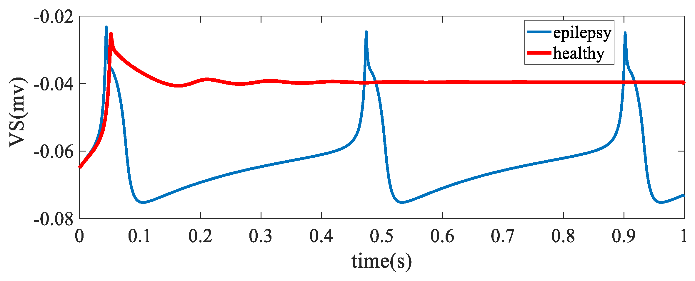
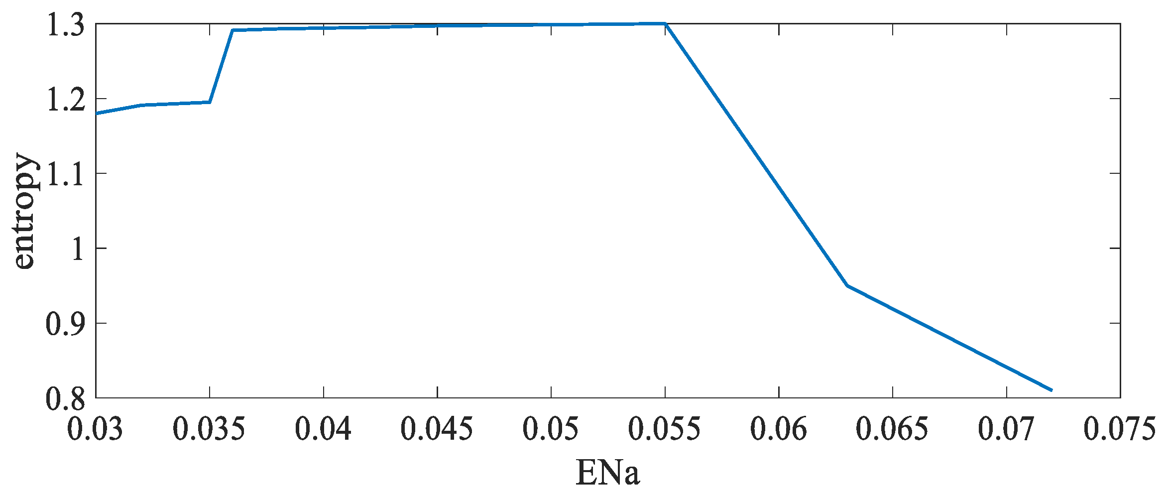
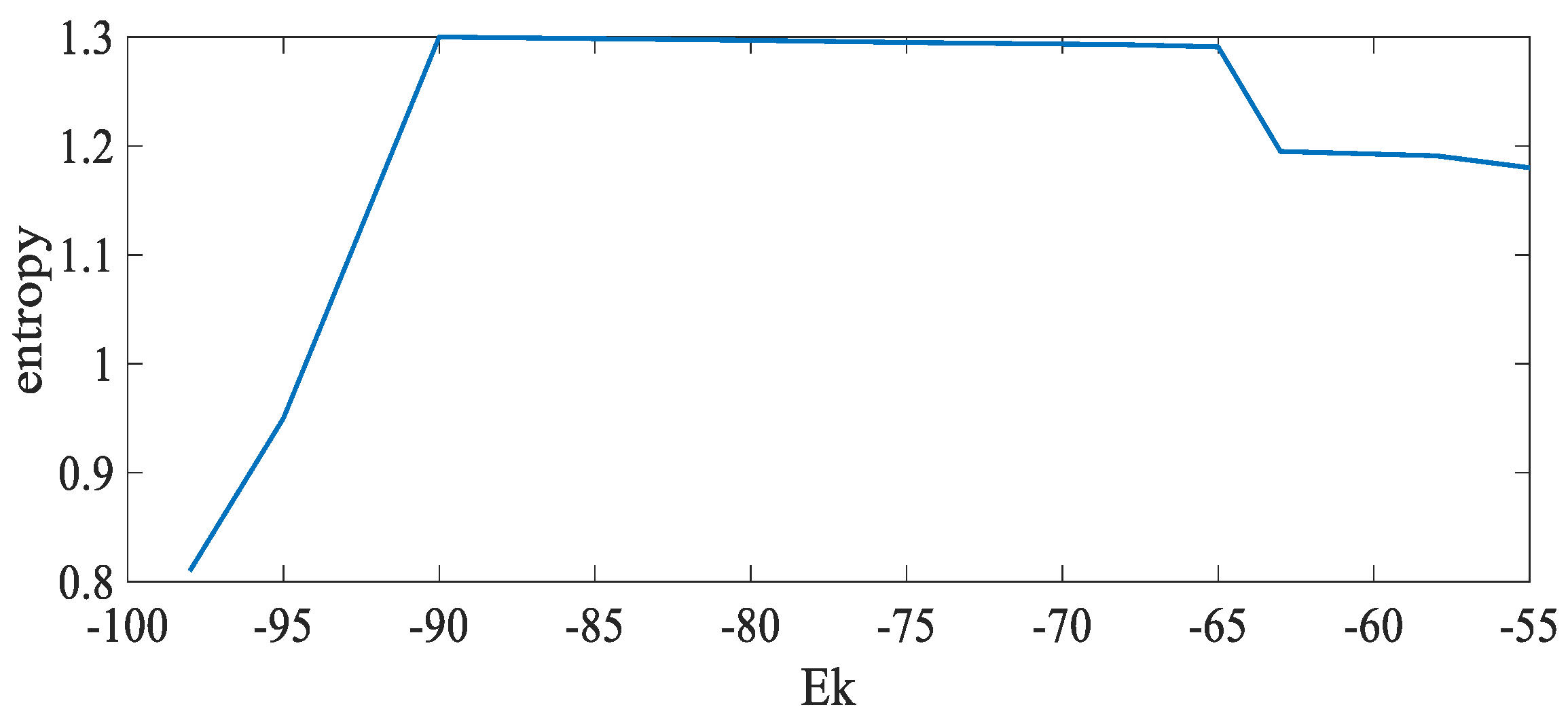
  • It analyzes the chaotic behavior of the PR model output (somatic membrane potential) using the entropy criterion.
  • It designs a TSMC approach which yields finite time converges of the system to the desired value, whilst ensuring chattering free dynamics.
  • An approach that relies on the barrier function, without needing any information about the boundary of perturbations, to adjust the sliding surface, decrease the error and further improve the system response.
The rest of the paper is organized as follows. Section 2 describes the two-compartmental (PR) model describing the neuron’s behaviors in the CA3 region of the brain. The behavior of the model is analyzed by entropy criteria in Section 3. The proposed adaptive barrier function terminal sliding mode controller is developed in Section 4. The simulation results are presented in Section 5. Finally, the conclusions are provided in Section 6.

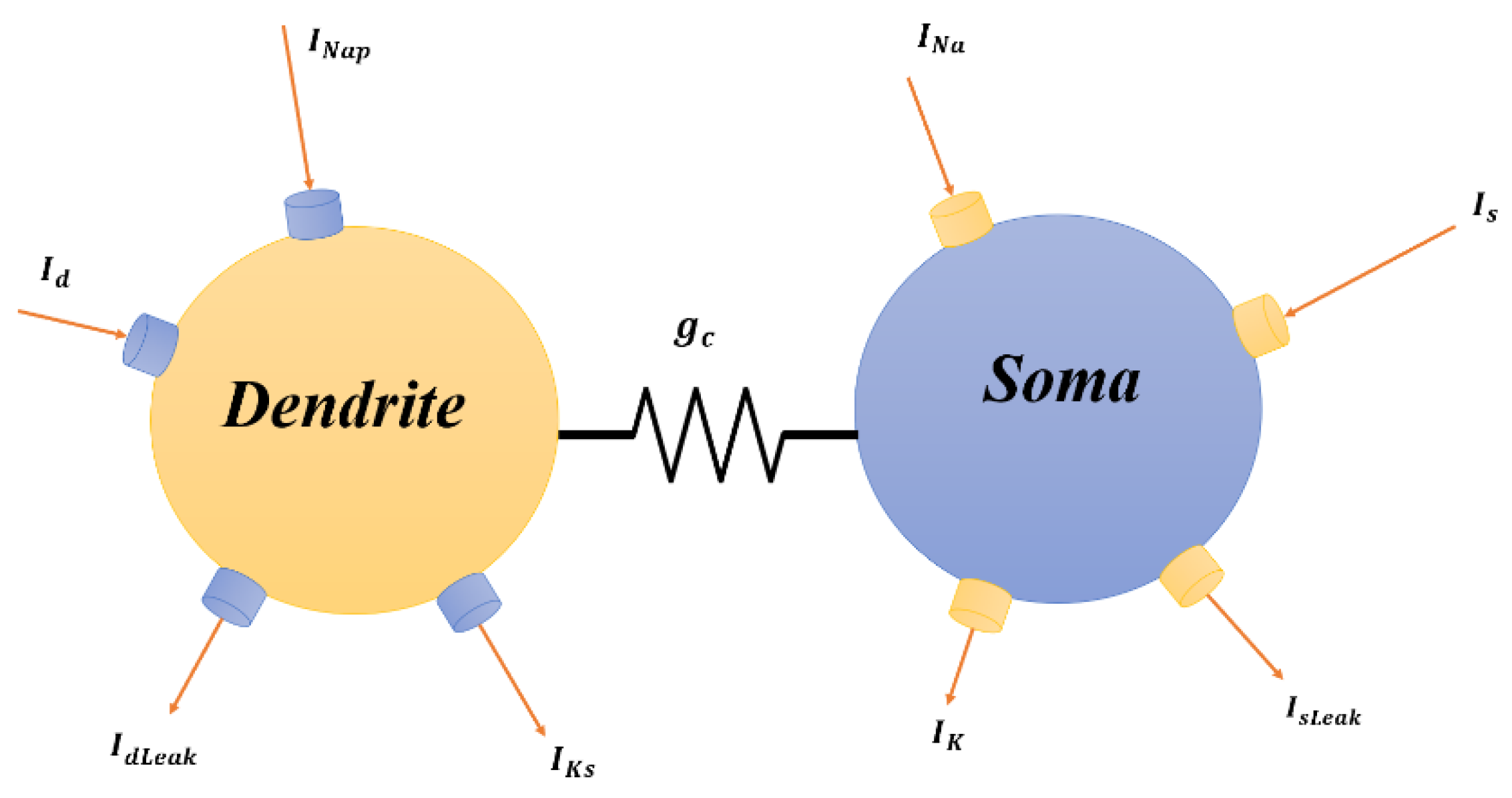
2. Two-Compartmental (PR) Model

The proposed model is a nonlinear and dynamic model that describes the neurons’ behaviors in the C A 3 region of the brain. This model consists of two parts and is shown in Figure 1.
A part of this model simulates the dendrite, whereas the other part simulates the axon. The two parts are separated by a conductor. Soma produces a spike. Dendrite is the other compartment that produces bursting responses Additionally, in Figure 1 currents entering and leaving the soma and dendrites are shown. In this model, V s   and   V d represent the membrane potential of the soma and dendrites, respectively. P represents the amount of space taken by the soma and C m is the membrane’s capacity.
The PR nonlinear model can be represented using the following nonlinear system [43,44].
V ˙ s = f ( x ) + u + δ x
V ˙ d = g ( x )
m ˙ = α m ( V s ) m ( α m ( V s ) + β m ( V s ) )
n ˙ = α n ( V s ) n ( α n ( V s ) + β n ( V s ) )
h ˙ = α h ( V s ) h ( α h ( V s ) + β h ( V s ) )
y = V s
where x = [ x 1 x 2 ] T denotes the vector of the system states; u is the control input; and y is the system output. The nonlinear functions f ( x ) ,   g ( x ) and δ x are chosen as follows:
f ( x ) = I N a I k I L e a k + I L i n k P + I s o m a
g ( x ) = I N a P I K S I L e a k I L i n k ( 1 P ) + I d e n d r i t e
δ x = Δ x V s + d
where Δ x V s represents system uncertainties and d denotes the external disturbances. Additionally, the variable δ x is bounded and its boundary is unknown.
The parameter values used in this paper are provided in [45] and are given in the Appendix A. The equations describing the currents of soma and dendrites are as follows:
I N a = g N a m 3 h   ( V s E N a )
I K = g k n 4 ( V s E K )
I L i n k = g c ( V d V s )
I N a P = g N a P l 3 ( V d V s )
I K S = g K S q ( V d E K )
I L e a k ( V s ) = g L ( V s E L )
I L e a k ( V d ) = g L ( V d E L )
The variables q ,   h ,   n follow the equations as follows:
d y d t = φ y ( y   ( V s ) y τ y ( V s ) )
If y = q ,   n ,   h , the amount of φ y is given by φ h = 3.3, φ n = 3.3 and φ q = 1. Time constant equations are given by:
y = α y α y   + β y ;   τ y = 1 α y + β y
where y = h ,   n
q ( V d ) = 1 / ( 1 + e x p ( V d + 35 ) / 6.5 )
τ q ( V d ) = 200 e x p ( ( V d + 55 ) / 30 ) + e x p ( ( V d + 55 ) / 30 )
l ( V d ) = 1 ( 1 + e x p ( ( V d + 57.7 ) / 7.7 ) )
m = α m / ( α m + β m )
The rate constant equations are given by:
α h ( V s ) = 0.07 e x p ( ( V s + 47 ) / 20 )
β h ( V s ) = 1 / ( e x p ( V s + 17 ) ) + 1 )
α n ( V s ) = 0.01 ( V s + 34 ) / ( e x p ( 0.1 ( V s + 34 ) ) 1 )
β n ( V s ) = 0.125   e x p ( ( V s + 44 ) / 80 )
α m ( V s ) = 0.1 ( V s + 31 ) / ( e x p ( V s + 31 ) ) 1 )
β m ( V s ) = 4   e x p ( ( V s + 56 ) / 18 )
The dynamic model produces different behavior patterns with different parameters. By selecting various pathological parameters, the applied current to the soma and dendrites will be different. The behavior of the soma membrane, while the two components are electrically coupled, in the epilepsy and healthy state is shown in Figure 2. The soma membrane potential is considered as the output of the system to control. When the seizure occurs, the electrical balance of the brain is lost and the membrane potential oscillates with high amplitude. In the healthy state, the range of oscillations of V s is reduced until it achieves the steady state. Changing the equilibrium potential ( E N a   &   E K ) , which also affects the current, changes the soma potential from the patient’s state to the healthy state.
It is clear that in the healthy state, periodic signals with high amplitudes are not observed.

3. Analysis of Entropy

The entropy criterion was introduced by Shannon in [46]. This criterion is a measure of the regularity or irregularity of the signal. Increasing the regularity in the signal increases the entropy criterion. Biologically, when the brain is in an epilepsy state, brain signals are more regular than in a healthy state [47,48]. It can be concluded that the entropy of the V s obtained in the healthy state is less than in the epileptic state. Entropy ( E n ) is defined by the discrete set of probabilities p i . If X is a set of discrete samples, entropy is defined as follows:
E n ( X ) = i = 1 n p ( x i ) l o g   p ( x i )
If x i ( i = 1 , 2 , 3 , , n ) and n is the number of samples, p ( x i ) is the probability of occurrence of x i . As seen in Figure 2, in epilepsy, the V s signal is oscillating and regular, but in the healthy state, the V s waveform does not have regularity and after a short time, it converges to its final value. Table 1 shows the E n of V s versus the different values of ( E N a   and     E k ) . As the E N a decreases and E k increases, the signal reaches its healthy state. In an epileptic state, entropy has its highest value.
For the epilepsy state, E N a = 0.05 and E k = 0.09 are selected. In Figure 3, E n changes are shown by the variation in E N a . In Figure 4, E n changes are shown by the variation in E k .

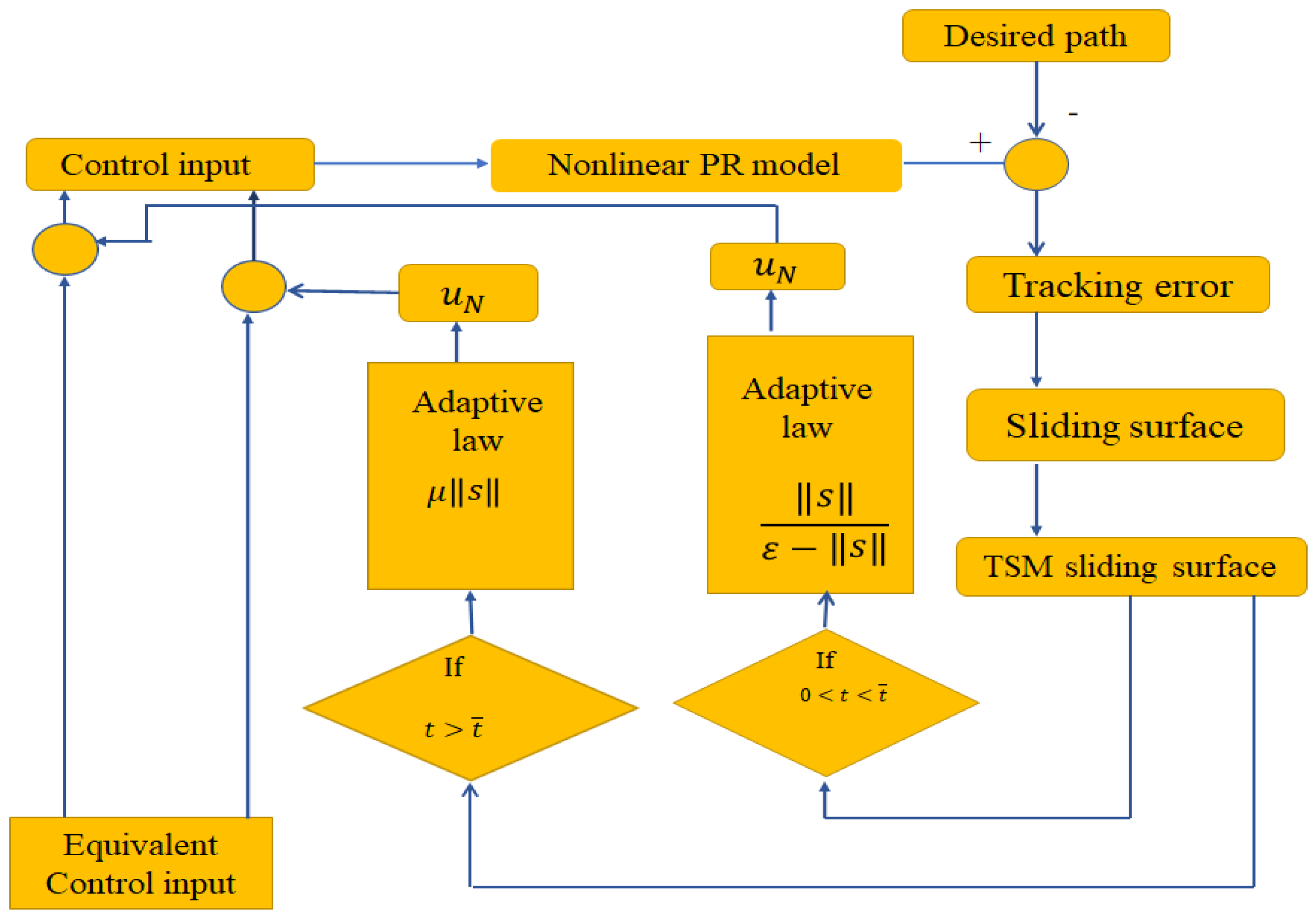
4. Adaptive Barrier Function Terminal Sliding Mode Control

Figure 5 shows the adaptive barrier function terminal sliding mode controller (ABTSMC) for controlling epilepsy, based on the PR model.
Assumption 1.
The δ x term is a bounded function with an unknown bound δ x m a x , with the following condition. The positive upper bound δ x m a x exists, but is an unknown value by
| δ x | δ x m a x
δ x m a x > 0
The epileptic soma potential ( V s ) is assumed to track the healthy desired reference V s d . Consider the following nonlinear system with external turbulences:
x ˙ 1 = x 2
x ˙ 2 = f ( x ) + B u ( t ) + δ x
where x 1 and x 2 are the states of the system (26) and f ( x ) is a nonlinear function.
The nonlinear TSMC surface can be expressed as follows [49,50,51]:
s = x 2 + λ x 1 p q
where λ > 0 is a constant and p and q are positive integers which satisfy the following conditions:
1 2 < p q < 1
The following equation is obtained by substituting (26) into the derivative (27).
s ˙ = f ( x ) + B u ( t ) + λ p q x 2 x 1 p q q + δ x
Lemma 1.
Given a positive-definite Lyapunov function V ( t ) , the derivative of V ( t ) must have the following inequality:
V ˙ ( t ) + α V 0  
where α is a positive parameter.
If the input of the control is expressed as follows:
u = u e q + u N
By using (26) and s ˙ = 0 , Equation (31) is written as:
u = B 1 ( f ( x ) + λ p q x 2 x 1 p q q + k s i g n ( s ) )
Define a positive-definite Lyapunov function as:
V ( t ) = 1 2 s 2
Deriving (33) with respect to time and using (29), one obtains:
V ˙ ( t ) = s ( f ( x ) + B u ( t ) + λ p q x 2 x 1 p q q + δ x )
By substituting the control law (32) in the above equation and considering Assumption 1, Lemma 1 is proven.
The nonlinear sliding surface (27) converges to the origin in the finite time. By considering s = 0 , we have:
d x 1 λ x 1 p q = λ d t
Integrating (35) from both sides yields:
x 1 ( t r ) 0 x 1 p q d x 1 = 0 t s λ d t
where t r = | s ( 0 ) | α
t s = q x 1 ( t r ) q p q λ ( q p )
The performance of the TSMC approach in the presence of external disturbance can further be improved by using an adaptive barrier function. By employing the barrier function, the control law can be defined as follows [52,53]:
u = B 1 ( f ( x ) + λ p q x 2 x 1 p q q + ( k + φ ^ ) s i g n ( s ) )
where
φ ^ ( t ) = { φ a                         0 < t < t ¯ φ p s d                               t > t ¯
t ¯ is defined as the time that trajectories are consolidated to the surroundings of the TSM sliding surface (27). The adaptation rule by positive semidefinite barrier functions is provided as:
{ φ a ˙ = μ s φ p s d = s ε s
where μ and ε are positive constants.
Using φ ^ ( t ) causes state trajectories to reach the neighborhood ε of the TSM sliding surface in t ¯ . For a time larger than t ¯ , φ ^ ( t ) is switched to the positive semidefinite part, which reduces the convergence region. The stability is analyzed in two statuses: one for the 0 < t < t ¯ condition and the other for t > t ¯ .
Theorem 1.
Consider the nonlinear system (26) and the nonlinear TSMC surface (27). The adaptive control law (38) with the adaptation condition φ ^ ( t ) = φ a from (39) satisfies the finite time tracking purpose of the states of nonlinear system (26).
Proof. 
Consider a Lyapunov function that is expressed as follows:
v 1 = 1 2 ( s T s + ζ 1 ( φ a φ ) 2 )
where ζ and φ are two positive constants.
The time derivative of v 1 is as follows:
v ˙ 1 = s T s ˙ + ζ 1 ( φ a φ ) φ ˙ a )
By placing (29) and φ a ˙ in the above equation, (43) is obtained
v ˙ 1 = s T ( f ( x ) + B u ( t ) + λ p q x 2 x 1 p q q + δ x ) + ( ζ 1 μ ( φ a φ ) s )
By substituting the adaptive control law in the above equation, we have:
v ˙ 1 = s T ( δ x ( φ ^ + k ) s i g n ( s ) ) + ( μ ζ 1 ( φ a φ ) s ) k s + s δ x s T φ a s i g n ( s ) + μ ζ 1 ( φ a φ ) s δ x s φ a s + μ ζ 1 ( φ a φ ) s ) + φ s φ s ( φ δ x ) s ( 1 μ ζ 1 ) ( φ a φ ) s
If φ δ x > 0 and μ ζ 1 < 1 , Equation (44) can be expressed as:
v ˙ 1 2 ( φ δ x ) s 2 2 ζ   ( 1 μ ζ 1 ) s φ a φ 2 ζ   m i n { 2 ( φ δ x ) , 2 ζ   ( 1 μ ζ 1 ) s } ( s 2 + φ a φ 2 ζ ) ρ 1 v 1 0.5 ρ 1 = m i n { 2 ( φ δ x ) , 2 ζ   ( 1 μ ζ 1 ) s } > 0
Theorem 2.
Consider the nonlinear system (26) and nonlinear TSMC surface (27). The adaptive control law (38) with the adaptation law φ ^ ( t ) = φ p s d from (39) can prove finite time tracking performance of the states of nonlinear system (26).
Proof. 
Consider a Lyapunov function as follows:
v 2 = 1 2 ( s T s + ( φ p s d φ p s d ( 0 ) ) 2 )
After differentiating from (46), we have:
v ˙ 2 = s T s ˙ + ( φ p s d φ p s d ( 0 ) ) φ ˙ p s d
By placing (29) and φ ( 0 ) = 0 in the above equation, (48) is obtain:
v ˙ 2 = s T ( f ( x ) + B u ( t ) + λ p q x 2 x 1 p q q + δ x ) + φ p s d φ ˙ p s d
By substituting the adaptive control law in (48), we have:
v ˙ 2 = s T { δ x ( φ p s d + k ) s i g n ( s ) } + φ p s d ε ( ε s ) 2 s i g n ( s ) s   ˙ k s + δ x s φ p s d s + φ p s d   ε ( ε s ) 2 s i g n ( s ) { δ x ( φ p s d + k ) i g n ( s ) } k ( s + φ p s d ε ( ε s ) 2 ) ( φ p s d δ x ) s ε ( ε s ) 2 { φ p s d δ x } φ p s d
If φ p s d > δ x and ε ( ε s ) 2 > 0 , Equation (49) can be expressed as:
v 2 ˙ 2 ( φ p s d δ x ) s 2 2   ε ( ε s ) 2   { φ p s d δ x } φ p s d 2 ( φ p s d δ x ) m i n { 1 ,   ε ( ε s ) 2 } ( s 2 + φ p s d 2 ) ρ 2 v 2 0.5 ρ 2 = 2 ( φ p s d δ x ) m i n { 1 ,   ε ( ε s ) 2 }

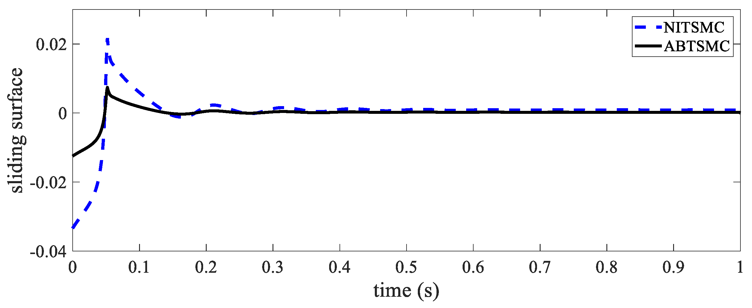
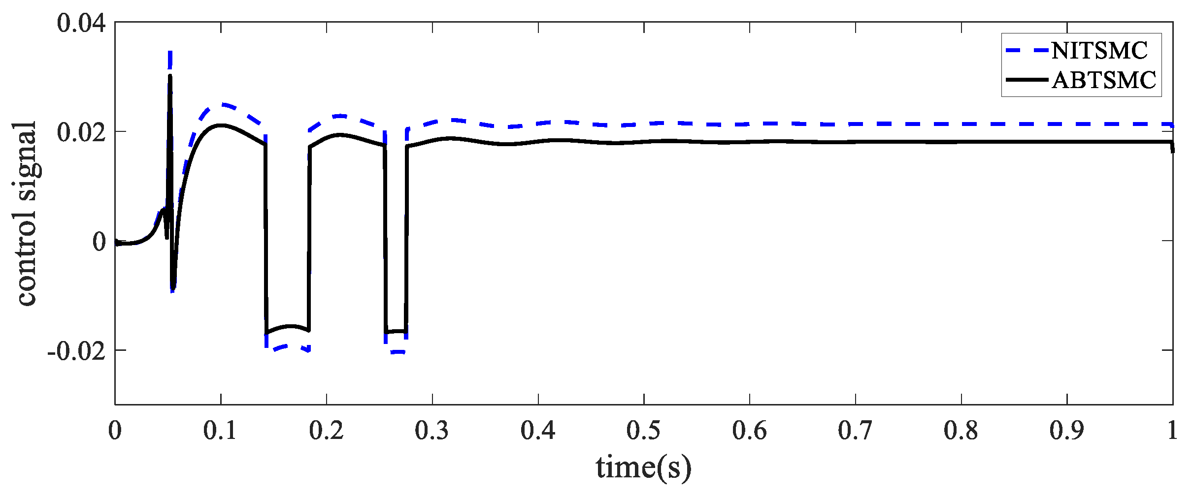
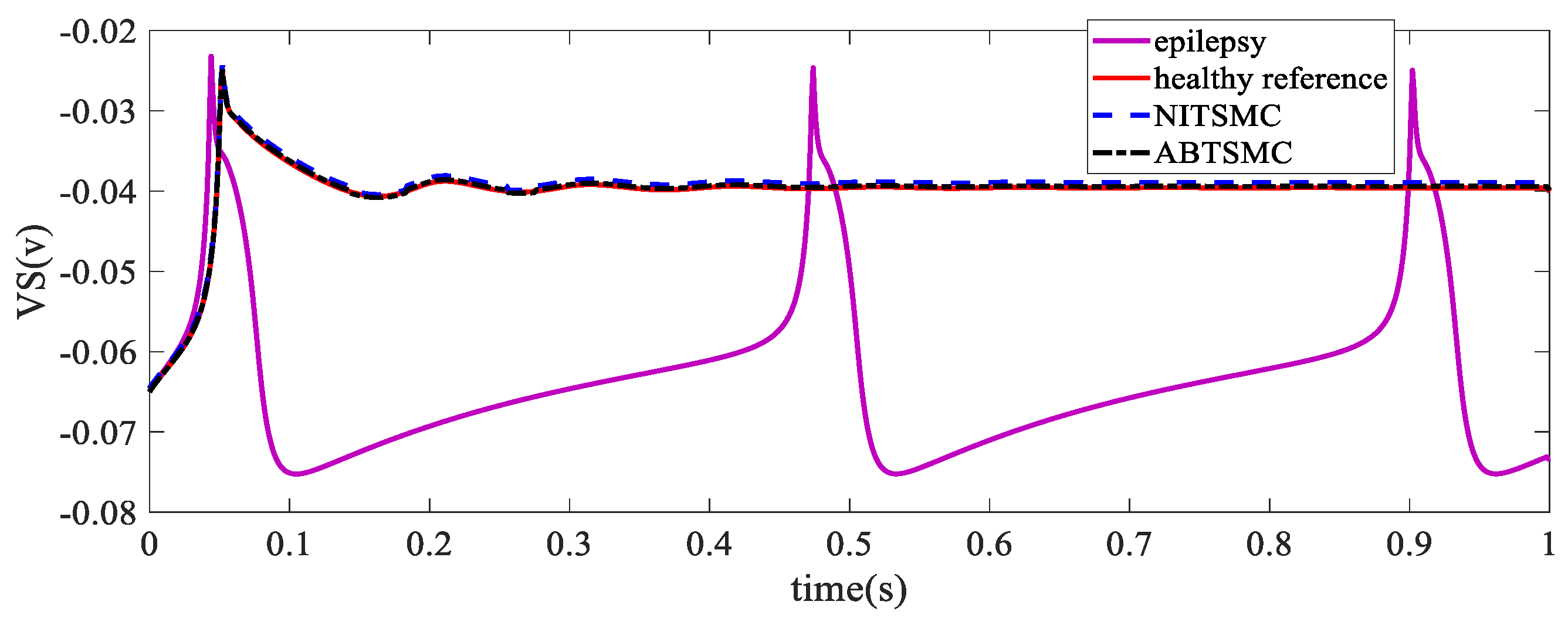
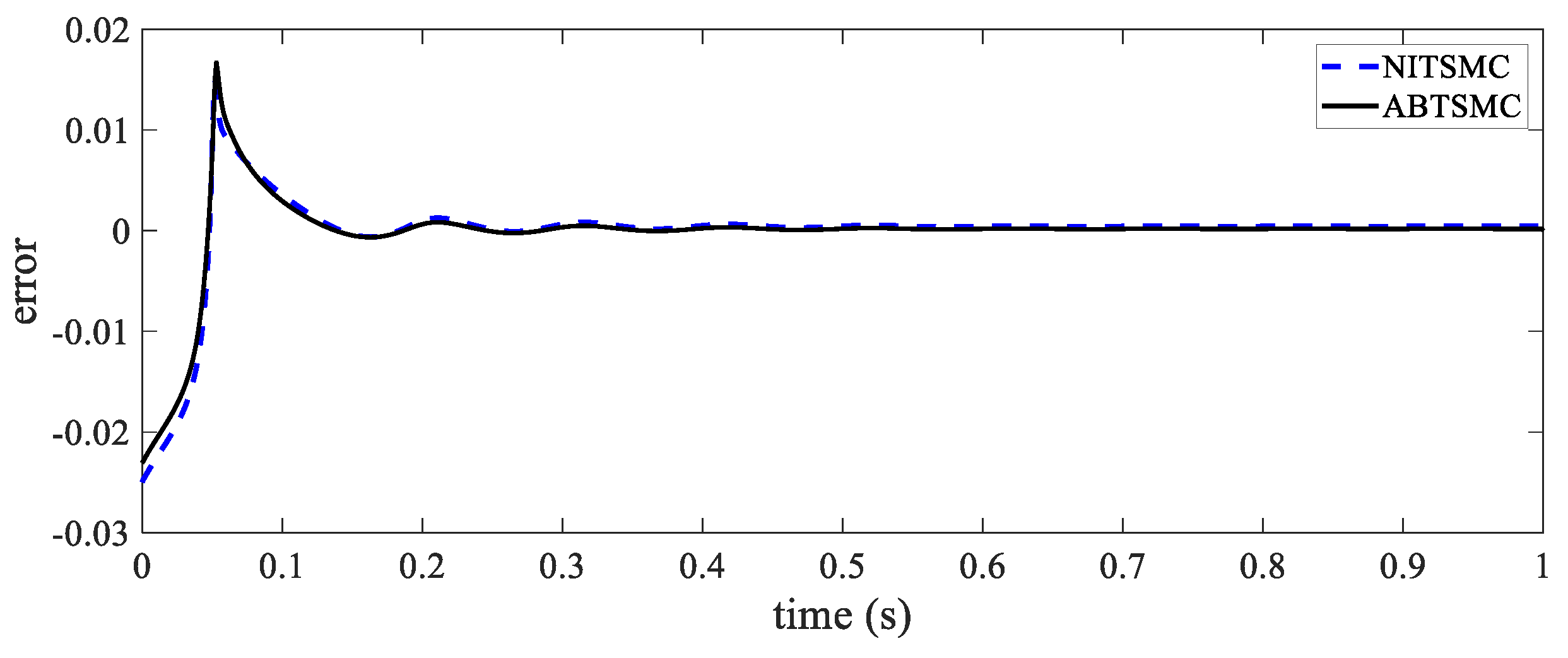
5. Simulation Results

In this section, the performance of the adaptive robust controller is analyzed using a simulation study. To demonstrate the ability of the proposed controller to control seizures, different patient modes were considered using different pathological parameters. The proposed approach is compared to the approach in [37], which employs a nonsingular integral terminal sliding mode (NITSMC). The dynamics of the sliding surfaces for both approaches are depicted in Figure 6.
The term p q is selected equal to 9 13 in (27). The control signals for both approaches are shown in Figure 7. Note that the (ABTSMC) control signal is simpler and has fewer ranges.
As shown in Figure 8, V s is the epileptic state after applying the ABTSM controller in the presence of disturbance and uncertainty, tracking the healthy state well. The proposed approach performance is compared with the approach proposed in [37]. The tracking error in the ABTSMC technique is less.
Mean square error (MSE), IAE and ISV criteria are examined in Table 2 and confirm the performance of the proposed method. The error of the proposed method is very small and close to zero. The error waveform after applying ABTSMC and NITSMC is shown in Figure 9.
All the obtained results confirm the performance of the proposed approach in the finite time convergence of the system outputs to the desired states and chattering-free dynamics.

6. Conclusions

This paper proposed a ABTSMC based on the PR model to control epileptic seizures. The approach can eliminate the uncertainty and external disturbance effects. This approach achieves three main objectives: (1) TSMC convergence to the reference value occurs in finite time, (2) chattering-free dynamics and (3) using the adaptive barrier function without needing any information about the boundary of disturbances decreases the error and further improves system response. The performance analysis and simulation results confirmed the effectiveness of this technique to control seizures. In our further work, we suggest using the hyperbolic tangent and fuzzy with adaptive barrier function higher sliding mode.

Author Contributions

Conceptualization, Z.M., M.T.V. and S.M.; formal analysis, S.M., T.R., Z.M. and M.T.V.; funding acquisition, T.R.; investigation, S.M., T.R., Z.M. and M.T.V.; methodology, Z.M. and S.M.; writing—original draft, Z.M., M.T.V. and S.M.; writing—review and editing and supervision, S.M., T.R., Z.M. and M.T.V. All authors have read and agreed to the published version of the manuscript.

Funding

This research was supported by Chiang Mai University.

Institutional Review Board Statement

Not applicable.

Informed Consent Statement

Not applicable.

Data Availability Statement

The data that support the findings of this study are available within the article.

Conflicts of Interest

The authors declare no conflict of interest.

Appendix A

The parameter values of the PR model are taken from [45] and are given in Table A1.
Table A1. Parameter values for the Pinsky–Rinzel model.
SymbolQuantityValueUnitSymbolQuantityValueUnit
E L a Equilibrium potential 65 mV   g c Conductance 1 mS cm 2
E N a Equilibrium potential 55 mV g N a P Conductance 0.12 mS cm 2
E K Equilibrium potential 90 mV g K S Conductance 0.7 mS cm 2
C m Membrane capacitance 1 μ F cm 2 g K Conductance 20 mS cm 2  
g L Conductance 0.18 mS cm 2 P Compartment coupling 0.15 _
g N a Conductance 55 mS cm 2

References

  1. Li, X.; Yang, H.; Yan, J.; Wang, X.; Yuan, Y.; Li, X. Seizure control by low-intensity ultrasound in mice with temporal lobe epilepsy. Epilepsy Res. 2019, 154, 1–7. [Google Scholar] [CrossRef] [PubMed]
  2. Magiorkinis, E.; Sidiropoulou, K.; Diamantis, A. Hallmarks in the history of epilepsy: Epilepsy in antiquity. Epilepsy Behav. 2010, 17, 103–108. [Google Scholar] [CrossRef]
  3. Sun, M.; Wang, F.; Min, T.; Zang, T.; Wang, Y. Prediction for high risk clinical symptoms of epilepsy based on deep learning algorithm. IEEE Access 2018, 6, 77596–77605. [Google Scholar] [CrossRef]
  4. Ge, M.; Guo, J.; Xing, Y.; Feng, Z.; Lu, W.; Ma, X.; Geng, Y.; Zhang, X. Transient reduction in theta power caused by interictal spikes in human temporal lobe epilepsy. In Proceedings of the 2017 39th Annual International Conference of the IEEE Engineering in Medicine and Biology Society (EMBC), Jeju Island, Korea, 11–15 July 2017; pp. 4256–4259. [Google Scholar]
  5. Nakahara, S.; Adachi, M.; Ito, H.; Matsumoto, M.; Tajinda, K.; van Erp, T.G. Hippocampal pathophysiology: Commonality shared by temporal lobe epilepsy and psychiatric disorders. Neurosci. J. 2018, 2018, 4852359. [Google Scholar] [CrossRef] [PubMed]
  6. Al-Otaibi, F.; Baeesa, S.S.; Parrent, A.G.; Girvin, J.P.; Steven, D. Surgical techniques for the treatment of temporal lobe epilepsy. Epilepsy Res. Treat. 2012, 2012, 374848. [Google Scholar] [CrossRef]
  7. Blair, R.D. Temporal lobe epilepsy semiology. Epilepsy Res. Treat. 2012, 2012, 751510. [Google Scholar] [CrossRef] [PubMed]
  8. Duncan, J.S.; Sander, J.W.; Sisodiya, S.M.; Walker, M.C. Adult epilepsy. Lancet 2006, 367, 1087–1100. [Google Scholar] [CrossRef]
  9. Sisodiya, S.; Lin, W.R.; Harding, B.; Squier, M.; Thom, M. Drug resistance in epilepsy: Expression of drug resistance proteins in common causes of refractory epilepsy. Brain 2002, 125, 22–31. [Google Scholar] [CrossRef]
  10. Bonelli, S.B.; Thompson, P.J.; Yogarajah, M.; Powell, R.H.; Samson, R.S.; McEvoy, A.W.; Symms, M.R.; Koepp, M.J.; Duncan, J.S. Memory reorganization following anterior temporal lobe resection: A longitudinal functional MRI study. Brain 2013, 136, 1889–1900. [Google Scholar] [CrossRef] [PubMed]
  11. Mansouri, A.; Fallah, A.; Valiante, T.A. Determining surgical candidacy in temporal lobe epilepsy. Epilepsy Res. Treat. 2012, 2012, 706917. [Google Scholar] [CrossRef] [PubMed]
  12. Zangiabadi, N.; Ladino, L.D.; Sina, F.; Orozco-Hernández, J.P.; Carter, A.; Téllez-Zenteno, J.F. Deep brain stimulation and drug-resistant epilepsy: A review of the literature. Front. Neurol. 2019, 10, 601. [Google Scholar] [CrossRef]
  13. Hodgkin, A.L.; Huxley, A.F. Currents carried by sodium and potassium ions through the membrane of the giant axon of Loligo. J. Physiol. 1952, 116, 449. [Google Scholar] [CrossRef]
  14. Izhikevich, E.M. Simple model of spiking neurons. IEEE Trans. Neural Netw. 2003, 14, 1569–1572. [Google Scholar] [CrossRef]
  15. Kriegeskorte, N.; Douglas, P.K. Cognitive computational neuroscience. Nat. Neurosci. 2018, 21, 1148–1160. [Google Scholar] [CrossRef]
  16. Liley, D.T.; Cadusch, P.J.; Wright, J.J. A continuum theory of electro-cortical activity. Neurocomputing 1999, 26, 795–800. [Google Scholar] [CrossRef]
  17. Pinsky, P.F.; Rinzel, J. Intrinsic and network rhythmogenesis in a reduced Traub model for CA3 neurons. J. Comput. Neurosci. 1994, 1, 39–60. [Google Scholar] [CrossRef]
  18. Suffczynski, P.; Kalitzin, S.; Da Silva, F.L. Dynamics of non-convulsive epileptic phenomena modeled by a bistable neuronal network. Neuroscience 2004, 126, 467–484. [Google Scholar] [CrossRef]
  19. Ullah, G.; Schiff, S.J. Tracking and control of neuronal Hodgkin-Huxley dynamics. Phys. Rev. E 2009, 79, 040901. [Google Scholar] [CrossRef]
  20. Chen, B.-S.; Li, C.-W. Robust observer-based tracking control of hodgkin-huxley neuron systems under environmental disturbances. Neural Comput. 2010, 22, 3143–3178. [Google Scholar] [CrossRef]
  21. Chen, S.; Yang, R. Control of repetitive firing in Hindmarsh-Rose model based on Krasovskii theorem. In Proceedings of the 2016 International Conference on Advanced Robotics and Mechatronics (ICARM), Macau, China, 18–20 August 2016; pp. 405–408. [Google Scholar]
  22. Soltan, A.; Xia, L.; Jackson, A.; Chester, G.; Degenaar, P. Fractional order PID system for suppressing epileptic activities. In Proceedings of the 2018 IEEE International Conference on Applied System Invention (ICASI), Chiba, Japan, 13–17 April 2018; pp. 338–341. [Google Scholar]
  23. Deng, B.; Li, G.; Wang, J.; Wei, X.; Su, F. Dynamic control of seizure states with input-output linearization method based on the Pinsky-Rinzel model. In Proceedings of the 2014 7th International Conference on Biomedical Engineering and Informatics, Fukuoka, Japan, 26–28 November 2014; pp. 425–430. [Google Scholar]
  24. Sinha, S.; Ditto, W.L. Controlling neuronal spikes. Phys. Rev. E 2001, 63, 056209. [Google Scholar] [CrossRef]
  25. Wei, W.; Wei, X.; Zuo, M.; Yu, T.; Li, Y. Seizure control in a neural mass model by an active disturbance rejection approach. Int. J. Adv. Robot. Syst. 2019, 16, 1729881419890152. [Google Scholar] [CrossRef]
  26. Selvaraj, P.; Sleigh, J.W.; Freeman, W.J.; Kirsch, H.E.; Szeri, A.J. Open loop optogenetic control of simulated cortical epileptiform activity. J. Comput. Neurosci. 2014, 36, 515–525. [Google Scholar] [CrossRef]
  27. Edwards, C.; Spurgeon, S. Sliding Mode Control: Theory and Applications; CRC Press: Boca Raton, FL, USA, 1998. [Google Scholar]
  28. Khalil, H.K. Nonlinear Systems Third Edition; Patience Hall: Hoboken, NJ, USA, 2002; Volume 115. [Google Scholar]
  29. Utkin, V.I. Sliding mode control design principles and applications to electric drives. IEEE Trans. Ind. Electron. 1993, 40, 23–36. [Google Scholar] [CrossRef]
  30. Rojsiraphisal, T.; Mobayen, S.; Asad, J.H.; Vu, M.T.; Chang, A.; Puangmalai, J. Fast terminal sliding control of underactuated robotic systems based on disturbance observer with experimental validation. Mathematics 2021, 9, 1935. [Google Scholar] [CrossRef]
  31. Mirzaei, A.; Ozgoli, S.; Jajarm, A.E. Chaotic analysis of the human brain cortical model and robust control of epileptic seizures using sliding mode control. Syst. Sci. Control Eng. Open Access J. 2014, 2, 216–227. [Google Scholar] [CrossRef]
  32. Mobayen, S. Design of LMI-based global sliding mode controller for uncertain nonlinear systems with application to Genesio’s chaotic system. Complexity 2015, 21, 94–98. [Google Scholar] [CrossRef]
  33. Mobayen, S. An LMI-based robust controller design using global nonlinear sliding surfaces and application to chaotic systems. Nonlinear Dyn. 2015, 79, 1075–1084. [Google Scholar] [CrossRef]
  34. Wu, Y.; Yu, X.; Man, Z. Terminal sliding mode control design for uncertain dynamic systems. Syst. Control Lett. 1998, 34, 281–287. [Google Scholar] [CrossRef]
  35. Zhihong, M.; Yu, X.H. Terminal sliding mode control of MIMO linear systems. IEEE Trans. Circuits Syst. I Fundam. Theory Appl. 1997, 44, 1065–1070. [Google Scholar] [CrossRef]
  36. Puangmalai, J.; Tongkum, J.; Rojsiraphisal, T. Finite-time stability criteria of linear system with non-differentiable time-varying delay via new integral inequality. Math. Comput. Simul. 2020, 171, 170–186. [Google Scholar] [CrossRef]
  37. Qian, M.; Zhang, Z.; Zhong, G.; Bo, C. A novel nonsingular integral terminal sliding mode control scheme in epilepsy treatment. Trans. Inst. Meas. Control 2022, 44, 1194–1204. [Google Scholar] [CrossRef]
  38. Rezvani Ardakani, S.; Mohammad-Ali-Nezhad, S.; Ghasemi, R. Epilepsy Control in a Combination of the Cortical and Optogenetic Models using Fixed Time Integral Super Twisting Sliding Mode Controller. Iran. J. Biomed. Eng. 2019, 13, 273–289. [Google Scholar]
  39. Chen, J.; Shuai, Z.; Zhang, H.; Zhao, W. Path following control of autonomous four-wheel-independent-drive electric vehicles via second-order sliding mode and nonlinear disturbance observer techniques. IEEE Trans. Ind. Electron. 2020, 68, 2460–2469. [Google Scholar] [CrossRef]
  40. Alattas, K.A.; Mofid, O.; Alanazi, A.K.; Abo-Dief, H.M.; Bartoszewicz, A.; Bakouri, M.; Mobayen, S. Barrier Function Adaptive Nonsingular Terminal Sliding Mode Control Approach for Quad-Rotor Unmanned Aerial Vehicles. Sensors 2022, 22, 909. [Google Scholar] [CrossRef]
  41. Mobayen, S.; Alattas, K.A.; Assawinchaichote, W. Adaptive continuous barrier function terminal sliding mode control technique for disturbed robotic manipulator. IEEE Trans. Circuits Syst. I Regul. Pap. 2021, 68, 4403–4412. [Google Scholar] [CrossRef]
  42. Obeid, H.; Fridman, L.M.; Laghrouche, S.; Harmouche, M. Barrier function-based adaptive sliding mode control. Automatica 2018, 93, 540–544. [Google Scholar] [CrossRef]
  43. Kepecs, A.; Wang, X.-J. Analysis of complex bursting in cortical pyramidal neuron models. Neurocomputing 2000, 32, 181–187. [Google Scholar] [CrossRef]
  44. Schwartzkroin, P.A. Role of the hippocampus in epilepsy. Hippocampus 1994, 4, 239–242. [Google Scholar] [CrossRef]
  45. Rahimian, E.; Zabihi, S.; Amiri, M.; Linares-Barranco, B. Digital implementation of the two-compartmental Pinsky–Rinzel pyramidal neuron model. IEEE Trans. Biomed. Circuits Syst. 2017, 12, 47–57. [Google Scholar] [CrossRef]
  46. Shannon, C.E. A mathematical theory of communication. Bell Syst. Tech. J. 1948, 27, 379–423. [Google Scholar] [CrossRef]
  47. Adeli, H.; Ghosh-Dastidar, S.; Dadmehr, N. A wavelet-chaos methodology for analysis of EEGs and EEG subbands to detect seizure and epilepsy. IEEE Trans. Biomed. Eng. 2007, 54, 205–211. [Google Scholar] [CrossRef]
  48. Mirzaei, A.; Ayatollahi, A.; Vavadi, H. Statistical analysis of epileptic activities based on histogram and wavelet-spectral entropy. J. Biomed. Sci. Eng. 2011, 4, 207. [Google Scholar] [CrossRef]
  49. Behnamgol, V.; Vali, A.R. Terminal sliding mode control for nonlinear systems with both matched and unmatched uncertainties. Iran. J. Electr. Electron. Eng. 2015, 11, 109–117. [Google Scholar]
  50. Feng, Y.; Yu, X.; Man, Z. Non-singular terminal sliding mode control of rigid manipulators. Automatica 2002, 38, 2159–2167. [Google Scholar] [CrossRef]
  51. Venkataraman, S.; Gulati, S. Control of nonlinear systems using terminal sliding modes. In Proceedings of the 1992 American Control Conference, Chicago, IL, USA, 24–26 June 1992. [Google Scholar]
  52. Alattas, K.A.; Mofid, O.; El-Sousy, F.F.; Alanazi, A.K.; Awrejcewicz, J.; Mobayen, S. Adaptive Nonsingular Terminal Sliding Mode Control for Performance Improvement of Perturbed Nonlinear Systems. Mathematics 2022, 10, 1064. [Google Scholar] [CrossRef]
  53. Mofid, O.; Mobayen, S.; Wong, W.-K. Adaptive terminal sliding mode control for attitude and position tracking control of quadrotor UAVs in the existence of external disturbance. IEEE Access 2020, 9, 3428–3440. [Google Scholar] [CrossRef]
Figure 1. Two-compartmental Pinsky–Rinzel model of C A 3 neurons.
Mathematics 10 02940 g001
Figure 2. Comparison between epilepsy state and healthy state.
Mathematics 10 02940 g002
Figure 3. Changing E n by the variation in E N a .
Mathematics 10 02940 g003
Figure 4. Changing E n by the variation in E k .
Mathematics 10 02940 g004
Figure 5. Control schematic of epilepsy based on the PR model.
Mathematics 10 02940 g005
Figure 6. Sliding surfaces of ABTSMC and NITSMC.
Mathematics 10 02940 g006
Figure 7. Comparison between ABTSMC and NITSMC control signals.
Mathematics 10 02940 g007
Figure 8. Tracking the healthy state of soma potential by ABTSM and NITSMC.
Mathematics 10 02940 g008
Figure 9. Comparison between ABTSMC and NITSMC error signals.
Mathematics 10 02940 g009
Table 1. Entropy for different parameters.
E K × 10 3 98 95 90 80 75 68 65 63 58 55
E N a 0.072 0.063 0.055 0.045 0.042 0.038 0.036 0.035 0.032 0.030
E n 0.8 0.95 1.3 1.297 1.295 1.293 1.291 1.195 1.191 1.181
Table 2. Comparison between two control methods.
ControllerMSEIAEISV (u)Chattering
Phenomenon
ABTSMC 0.01475 1.132 2.138 No
Method [37] 0.02095 1.967 3.792 No
Publisher’s Note: MDPI stays neutral with regard to jurisdictional claims in published maps and institutional affiliations.

