
Theoretical Model for Nonlinear Long Waves over a Thin Viscoelastic Muddy Seabed

Abstract
:1. Introduction
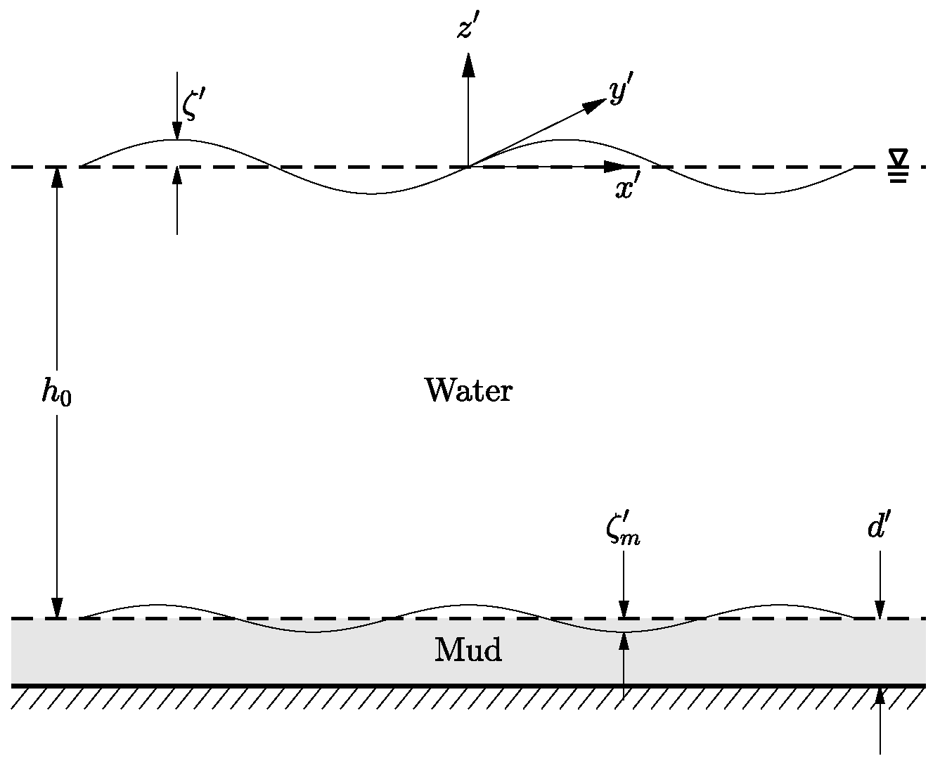
2. Formulations
2.1. Assumptions and Simplifications
2.2. Water Layer
2.3. Muddy Seabed
2.4. A Linear Viscoelastic Muddy Seabed
3. Examples and Discussions
3.1. Model Equations for the Wave-Mud Problem
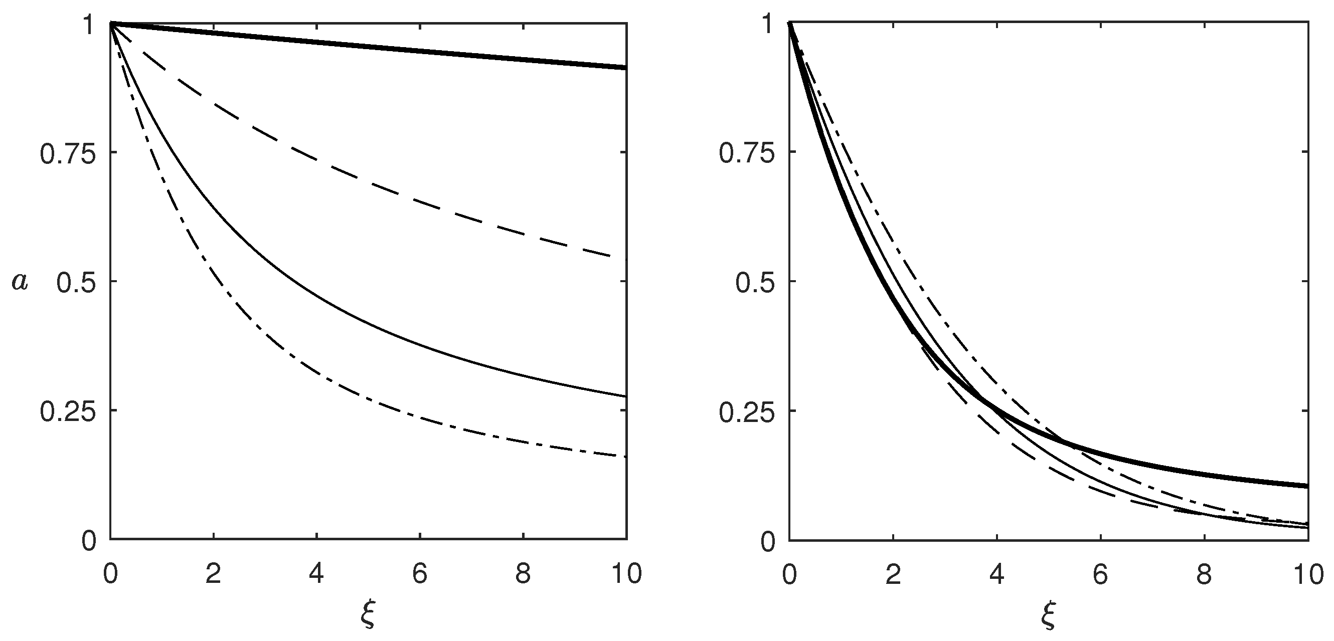
3.2. Linear Progressive Waves with Mud at Elastic or Viscous Limit
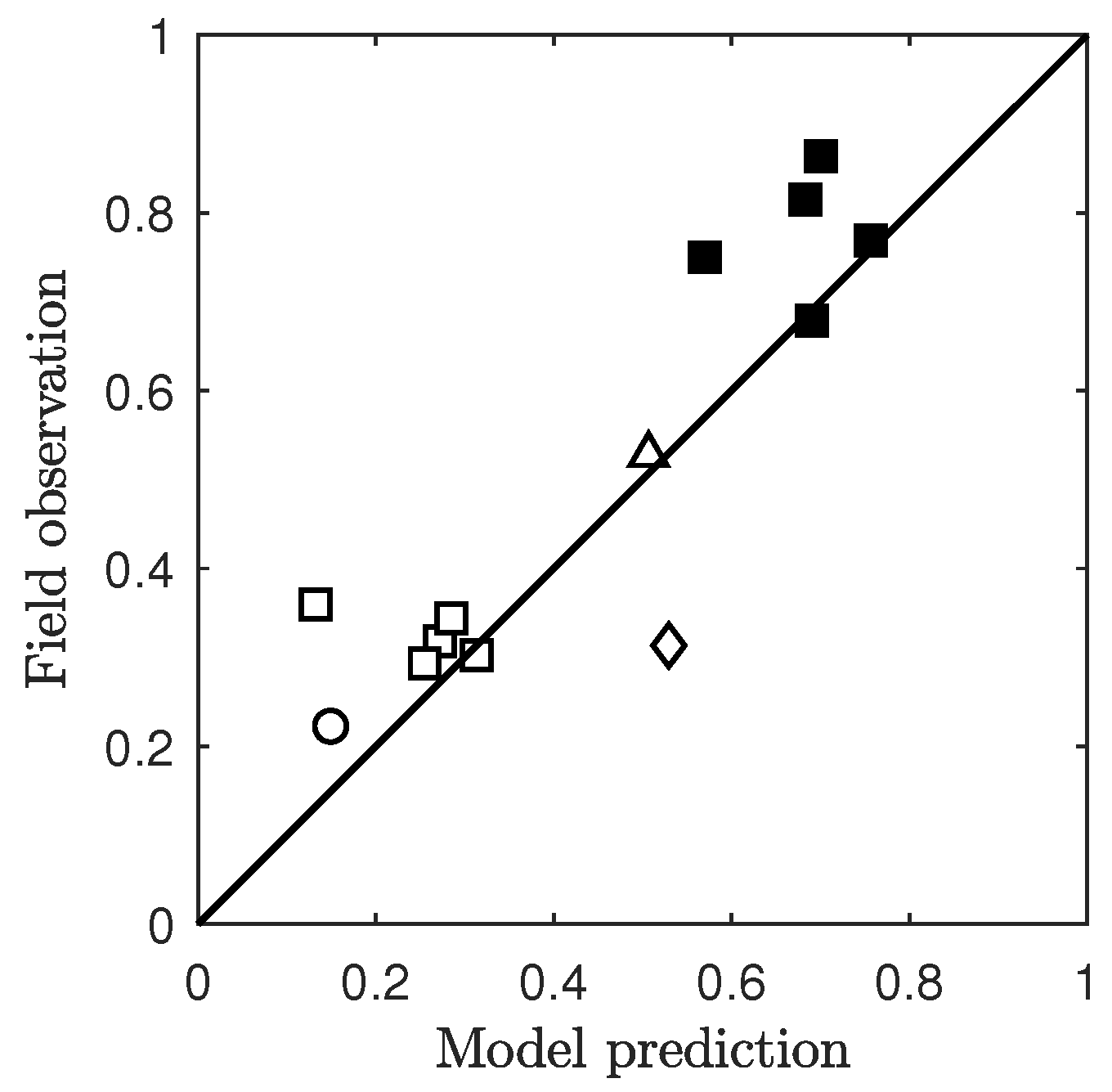
3.3. Comparisons with Field Observations
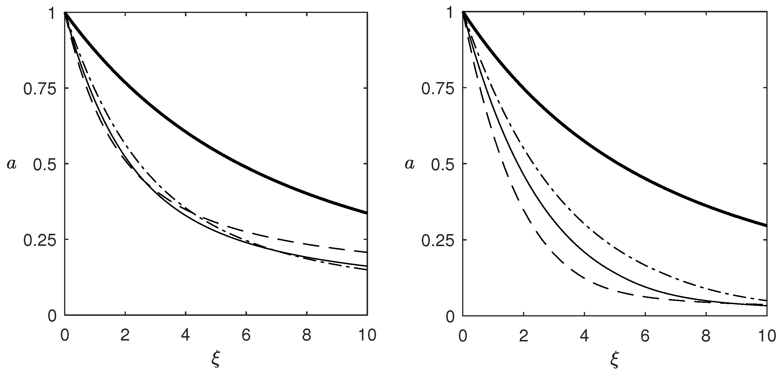
3.4. Effects of Mud Properties
4. Concluding Remarks
- Maximum wave damping occurs when the thickness of mud is about the same as the typical boundary layer thickness;
- A viscoelastic seabed is more efficient in wave damping than a Newtonian fluid mud, as elastic oscillation enhances the wave amplitude attenuation;
- The increase in elasticity in a viscoelastic seabed only has significant impacts on amplitude attenuation when the dimensionless mud thickness is larger.
Funding
Institutional Review Board Statement
Informed Consent Statement
Acknowledgments
Conflicts of Interest
References
- Gade, H.G. Effects of a non-rigid, impermeable bottom on plane surface waves in shallow water. J. Mar. Res. 1958, 16, 61–82. [Google Scholar]
- Tubman, M.W.; Suhayda, J.N. Wave action and bottom movements in fine sediments. In Proceedings of the 15th Coastal Engineering Conference, Honolulu, HI, USA, 11–17 July 1976; pp. 1168–1183. [Google Scholar]
- Elgar, S.; Raubenheimer, B. Wave dissipation by muddy seafloors. Geophys. Res. Lett. 2008, 35, L07611. [Google Scholar] [CrossRef] [Green Version]
- Wells, J.T.; Coleman, J.M. Physical processes and fine-grained sediment dynamics, Coast of Surinam, South America. J. Sediment. Petrol. 1981, 51, 1053–1068. [Google Scholar]
- Mathew, J. Wave–Mud Interaction in Mudbanks. Ph.D. Dissertation, Cochin University of Science and Technology, Cochin, India, 1992. [Google Scholar]
- Rogers, W.E.; Holland, K.T. A study of dissipation of wind-waves by mud at Cassino Beach, Brazil: Prediction and inversion. Cont. Shelf Res. 2009, 29, 676–690. [Google Scholar] [CrossRef]
- Foda, M.A. Sea floor dynamics. In Advances in Coastal and Ocean Engineering; Liu, P.L.-F., Ed.; World Scientific: Singapore, 1995; pp. 77–123. [Google Scholar]
- Mei, C.C.; Krotov, M.; Huang, Z.; Huhe, A. Short and long waves over a muddy seabed. J. Fluid Mech. 2010, 643, 33–58. [Google Scholar] [CrossRef] [Green Version]
- Dalrymple, R.A.; Liu, P.L.-F. Waves over soft muds: A two layer model. J. Phys. Oceanogr. 1978, 8, 1121–1131. [Google Scholar] [CrossRef] [Green Version]
- Liu, P.L.-F.; Chan, I.-C. On long-wave propagation over a fluid-mud seabed. J. Fluid Mech. 2007, 579, 467–480. [Google Scholar] [CrossRef]
- Mallard, W.W.; Dalrymple, R.A. Water waves propagating over a deformable bottom. In Proceedings of the 9th Offshore Technology Conference, Houston, TX, USA, 2–5 May 1977. OTC-2895-MS. [Google Scholar]
- Yamamoto, T.; Koning, H.L.; Sellmeigher, H.; Hijum, E.V. On the response of poro-elastic bed to water waves. J. Fluid Mech. 1978, 87, 193–206. [Google Scholar] [CrossRef]
- MacPherson, H. The attenuation of water waves over a non-rigid bed. J. Fluid Mech. 1980, 97, 721–742. [Google Scholar] [CrossRef]
- Ng, C.-O. Water waves over a muddy bed: A two-layer Stokes’ boundary layer model. Coast. Eng. 2000, 40, 221–242. [Google Scholar] [CrossRef]
- Liu, P.L.-F.; Chan, I.-C. A note on the effects of a thin visco-elastic mud layer on small amplitude water-wave propagation. Coast. Eng. 2007, 54, 233–247. [Google Scholar] [CrossRef]
- Mei, C.C.; Liu, K.-F. A Bingham-plastic model for a muddy seabed under long waves. J. Geophys. Res. 1987, 92, 14581–14594. [Google Scholar] [CrossRef]
- Liu, K.-F.; Mei, C.C. Effects of wave-induced friction on a muddy seabed modelled as a Bingham-plastic fluid. J. Coast. Res. 1989, 5, 777–789. [Google Scholar]
- Park, Y.S.; Liu, P.L.-F.; Clark, S.J. Viscous flows in a muddy seabed induced by a solitary wave. J. Fluid Mech. 2008, 598, 383–392. [Google Scholar] [CrossRef]
- Jiang, F.; Mehta, A.J. Mudbanks of the southwest coast of India. Part IV. Mud viscoelastic priperties. J. Coast. Res. 1995, 11, 918–926. [Google Scholar]
- Malvern, L.E. Introduction to the Mechanics of a Continuous Medium; Prentice Hall: Hoboken, NJ, USA, 1969; pp. 306–327. [Google Scholar]
- Mei, C.C. The Applied Dynamics of Ocean Surface Waves; World Scientific: Singapore, 1989; pp. 504–511. [Google Scholar]
- Lynett, P.J. A Multi-Layer Approach to Modeling Generation, Propagation, and Interaction of Water Waves. Ph.D. Dissertation, Cornell University, Ithaca, NY, USA, 2002. [Google Scholar]
- Soltanpour, M.; Haghshenas, S.A. Fluidization and representative wave transformation on muddy beds. Cont. Shelf Res. 2009, 29, 666–675. [Google Scholar] [CrossRef]
- Dean, R.G.; Dalrymple, R.A. Water Wave Mechanics for Engineers and Scientists; World Scientific: Singapore, 1991; pp. 262–268. [Google Scholar]
- Maa, J.P.-Y.; Mehta, A.J. Mud erosion by waves: A laboratory study. Cont. Shelf Res. 1987, 7, 1269–1284. [Google Scholar] [CrossRef]
- Traykovski, P.; Geyer, W.R.; Irish, J.D.; Lynch, J.F. The role of wave-induced density-driven fluid mud flows for cross-shelf transport on the Eel River continental shelf. Cont. Shelf Res. 2000, 20, 2113–2140. [Google Scholar] [CrossRef]
- Ng, C.-O.; Zhang, X. Mass transport in water waves over a thin layer of soft viscoelastic mud. J. Fluid Mech. 2007, 573, 105–130. [Google Scholar] [CrossRef] [Green Version]

| (kg/m) | (kg/m) | (m/s) | (N/m) | h (m) | d (m) | |
|---|---|---|---|---|---|---|
| TS76 , ∆ | 1000 | 1250 | 0.5 | 500 | 19.2 | 0.85 |
| WC81 , ☐ | 1000 | 1250 | 0.5 | 500 | 8.7 | 0.5 |
| WC81 , ■ | 1000 | 1250 | 0.5 | 500 | 5.8 | 0.25 |
| M92 , ◇ | 1030 | 1230 | 0.5 | 500 | 10 | 1.2 |
| RH09 , ○ | 1000 | 1310 | 0.0076 | 500 | 15 | 0.4 |
Publisher’s Note: MDPI stays neutral with regard to jurisdictional claims in published maps and institutional affiliations. |
© 2022 by the author. Licensee MDPI, Basel, Switzerland. This article is an open access article distributed under the terms and conditions of the Creative Commons Attribution (CC BY) license (https://creativecommons.org/licenses/by/4.0/).
Share and Cite
Chan, I.-C. Theoretical Model for Nonlinear Long Waves over a Thin Viscoelastic Muddy Seabed. Mathematics 2022, 10, 2715. https://doi.org/10.3390/math10152715
Chan I-C. Theoretical Model for Nonlinear Long Waves over a Thin Viscoelastic Muddy Seabed. Mathematics. 2022; 10(15):2715. https://doi.org/10.3390/math10152715
Chicago/Turabian StyleChan, I-Chi. 2022. "Theoretical Model for Nonlinear Long Waves over a Thin Viscoelastic Muddy Seabed" Mathematics 10, no. 15: 2715. https://doi.org/10.3390/math10152715
APA StyleChan, I.-C. (2022). Theoretical Model for Nonlinear Long Waves over a Thin Viscoelastic Muddy Seabed. Mathematics, 10(15), 2715. https://doi.org/10.3390/math10152715