Progress towards Analytically Optimal Angles in Quantum Approximate Optimisation

Abstract

The quantum approximate optimisation algorithm is a p layer, time variable split operator method executed on a quantum processor and driven to convergence by classical outer-loop optimisation. The classical co-processor varies individual application times of a problem/driver propagator sequence to prepare a state which approximately minimises the problem’s generator. Analytical solutions to choose optimal application times (called parameters or angles) have proven difficult to find, whereas outer-loop optimisation is resource intensive. Here we prove that the optimal quantum approximate optimisation algorithm parameters for $p=1$ layer reduce to one free variable and in the thermodynamic limit, we recover optimal angles. We moreover demonstrate that conditions for vanishing gradients of the overlap function share a similar form which leads to a linear relation between circuit parameters, independent of the number of qubits. Finally, we present a list of numerical effects, observed for particular system size and circuit depth, which are yet to be explained analytically.

1. Introduction

The field of quantum algorithms has dramatically transformed in the last few years due to the advent of a quantum to classical feedback loop: a fixed depth quantum circuit is adjusted to minimise a cost function. This approach partially circumvents certain limitations such as variability in pulse timing and requires shorter depth circuits at the cost of outer-loop training [1,2,3,4,5,6]. The most studied algorithm in this setting is the quantum approximate optimisation algorithm (QAOA) [7] which was developed to approximate solutions to combinatorial optimisation problem instances [8] i.e., MAX-k-SAT [9,10], MAX-Cut [7,11,12,13,14,15,16], and MAX-k-Colorable-Subgraph [17] instances. The algorithm has certain real-world applications, including finances [18] and might prove useful for general constraint optimisation [19].

The setting of QAOA is that of n qubits: states are represented as vectors in $V_n={\left[{\mathbb{C}}^2\right]}^{\otimes n}$. We are given a non-negative Hamiltonian $P\in {\mathrm{herm}}_{\mathbb{C}}\left(V_n\right)$ and we seek the normalised ground vector $|t\rangle \in \underset{\varphi \in {\{0,1\}}^n}{\mathrm{arg\; min}}\langle \varphi |P|\varphi \rangle$.

QAOA might be viewed as a (time-variable fixed-depth) quantum split operator method. We let $\mathcal{V}\left(\gamma \right)$ be the propagator of P applied for time $\gamma$. We consider a second propagator $\mathcal{U}\left(\beta \right)$ generated by applying a yet-to-be-defined Hamiltonian $H_x$ for time $\beta$. We start off in the equal superposition state ${|+\rangle }^{\otimes n}=2^{-n/2}{(|0\rangle +|1\rangle )}^{\otimes n}$ and form a p-depth $\mathcal{U}$, $\mathcal{V}$ sequence:

$$\begin{array}{c}\hfill |g_p{(\mathbf{\gamma },\mathbf{\beta })|}^2=|\langle t|{\mathsf{\Pi }}_{k=1}^p\left[\mathcal{U}\left({\beta }_k\right)\mathcal{V}\left({\gamma }_k\right)\right]|+{\rangle }^{\otimes n}{|}^2.\end{array}$$

(1)

The time of application of each propagator is varied to maximise preparation of the state t. Finding $\mathbf{\gamma },\mathbf{\beta }$ to maximise $|g_p(\mathbf{\gamma },\mathbf{\beta })|$ has shown to be cumbersome. Even lacking such solutions, much progress has been made.

Recent milestones include experimental demonstration of $p=3$ depth QAOA (corresponding to six tunable parameters) using a twenty three qubits [1] superconducting processor, universality results [20,21], as well as several results that aid and improve on the original implementation of the algorithm [11,12,17]. Towards practical realisation of the QAOA, trapped ion-based quantum computers have recently shown promising results, including demonstrations on up to forty qubits [2] and the potential to realise arbitrary combinatorial optimisation problems with all to all connectivity based on hardware-inspired modifications [22]. Although QAOA exhibits provable advantages such as recovering a near-optimal query complexity in Grover’s search [23] and offers a pathway towards quantum advantage [13], several limitations have been discovered for low depth QAOA [9,24,25].

In the setting of maximum-constraint satisfiability (e.g., minimizing a Hamiltonian representing a function of type $f:{\{0,1\}}^n\to {\mathbb{R}}_{+}$), it has been shown that underparameterisation of QAOA sequences can be induced by increasing a problem instances constraint to variable ratio [9]. This effect persists in graph minimisation problems [26]. While this effect is perhaps an expected limitation of the quantum algorithm, parameter concentrations and noise-assisted training add a degree of optimism. QAOA exhibits parameter concentrations, in which training for some fraction of $\omega <n$ qubits provides a training sequence for n qubits [27]. Moreover, whereas layerwise training saturates for QAOA in which the algorithm plateaus and fails to reach the target, local coherent noise recovers layerwise training robustness [28]. Both concentrations and noise-assisted training imply a reduction in computational resources required in outer-loop optimisation.

Exact solutions to find the optimal parameters for QAOA have only been possible in special cases including, e.g., fully connected graphs [14,15,16] and projectors [27]. A general analytical approach which would allow for (i) calculation of optimal parameters, (ii) estimation of the critical circuit depth and (iii) performance guarantees for fixed depth remains open.

Here we prove that optimal QAOA parameters for $p=1$ are related as ${\gamma }_1=\pi -2{\beta }_1$ and in the thermodynamic limit, we recover optimality as ${\beta }_{1}n\to \pi$ and ${\gamma }_1\to \pi$. We moreover demonstrate that conditions for vanishing gradients of the overlap function share a similar form which leads to a linear relation between circuit parameters, independent of the number of qubits. We hence devise an additional means to recover parameter concentrations [27] analytically. Finally, we present a list of numerical effects, observed for particular system size and circuit depth, which are yet to be explained analytically.

2. State Preparation with QAOA

We consider an n-qubit complex vector space $V_n={\left[{\mathbb{C}}^2\right]}^{\otimes n}\cong {\mathbb{C}}^{2^n}$ with fixed standard computational basis $B_n={\{|0\rangle ,|1\rangle \}}^{\otimes n}$. For an arbitrary target state $|t\rangle \in B_n$ (equivalently $|t\rangle ,t\in {\{0,1\}}^{\times n}$) we define propagators

$$\begin{array}{c}\hfill \mathcal{U}\left(\beta \right)\equiv e^{-i\beta H_x},\mathcal{V}\left(\gamma \right)\equiv e^{-i\gamma P},\end{array}$$

(2)

where $P=|t\rangle \langle t|$ and $H_x={\sum }_{j=1}^n{X}_j$ is the one-body mixer Hamiltonian with $X_j$ the Pauli matrix acting non-trivially on the j-th qubit. Here we focus on the state preparation, thus choosing the problem Hamiltonian to be a projector ($P^2=P$) on an arbitrary bit string $|t\rangle$. We note that while the projector has only two energy levels, the effective Hamiltonian of the whole QAOA sequence has up to $n+1$ distinct energy levels. In such settings, the propagator $\mathcal{V}\left(\gamma \right)$ acting on a superposition adds a phase $-\gamma$ to the component $|t\rangle$, while the propagator $\mathcal{U}\left(\beta \right)$ mixes the components’ amplitudes.

A p-depth (p layer) QAOA circuit prepares a quantum state $|\psi \rangle$ as:

$$\begin{array}{c}\hfill |{\psi }_p(\mathbf{\gamma },\mathbf{\beta })\rangle =\prod _{k=1}^p\left[\mathcal{U}\left({\beta }_k\right)\mathcal{V}\left({\gamma }_k\right)\right]|+{\rangle }^{\otimes n},\end{array}$$

(3)

where ${\gamma }_k\in [0,2\pi )$, ${\beta }_k\in [0,\pi )$. The optimisation task is to determine QAOA optimal parameters for which the state prepared in (3) achieves maximum absolute value of the overlap $g_p(\mathbf{\gamma },\mathbf{\beta })=\langle t|{\psi }_p(\mathbf{\gamma },\mathbf{\beta })\rangle$ with the target $|t\rangle$. In other words, we search for

$$\begin{array}{c}\hfill ({\mathbf{\gamma }}_{opt},{\mathbf{\beta }}_{opt})\in \arg \underset{\mathbf{\gamma },\mathbf{\beta }}{\max }\left|g_p(\mathbf{\gamma },\mathbf{\beta })\right|.\end{array}$$

(4)

Note that the problem is equivalent to the minimisation of the ground state energy of Hamiltonian $P^{\perp }= ⊮- |t\rangle \langle t|$,

$$\underset{\mathbf{\gamma },\mathbf{\beta }}{\min }\langle {\psi }_p(\mathbf{\gamma },\mathbf{\beta })|P^{\perp }|{\psi }_p(\mathbf{\gamma },\mathbf{\beta })\rangle =1-\underset{\mathbf{\gamma },\mathbf{\beta }}{\max }{\left|g_p(\mathbf{\gamma },\mathbf{\beta })\right|}^2.$$

(5)

Remark 1 (Inversion symmetry).

Under the affine transformation

$$\begin{array}{c}\hfill (\gamma ,\beta )\to (2\pi -\gamma ,\pi -\beta )\end{array}$$

(6)

the absolute value of the overlap remains invariant as $g_p\to {(-1)}^n{g}_p^{\ast }$. Therefore, this narrows the search space to ${\gamma }_k\in [0,\pi )$, ${\beta }_k\in [0,\pi )$, whereas maximums inside the restricted region determine maximums in the composite space using Equation (6).

Proposition 1 (Overlap invariance).

The overlap function $g_p(\mathbf{\gamma },\mathbf{\beta })$ is invariant with respect to $|t\rangle \in B_n$.

Proof. 

Each $|t\rangle =|t_1{t}_2\dots t_n\rangle \in B_n$ determines a unitary operator $U=U^{†}={⨂}_{j=1}^n{X}_j^{t_j}.$ Hence, we have

$$\begin{array}{ll}{g}_p(\mathbf{\gamma },\mathbf{\beta })=& \langle \mathbf{0}|U^{†}{\displaystyle \prod _{k=1}^p}{e}^{-i{\beta }_k{H}_x}{e}^{-i{\gamma }_{k}U(|\mathbf{0}\rangle \langle \mathbf{0}|)U^{†}}|+{\rangle }^{\otimes n}\hfill \\ \hfill =& \langle \mathbf{0}|U^{†}{\displaystyle \prod _{k=1}^p}{e}^{-i{\beta }_k{H}_x}\left[U{e}^{-i{\gamma }_k(|\mathbf{0}\rangle \langle \mathbf{0}|)}{U}^{†}\right]|+{\rangle }^{\otimes n}\hfill \\ \hfill =& \langle \mathbf{0}|{\displaystyle \prod _{k=1}^p}{e}^{-i{\beta }_k{H}_x}{e}^{-i{\gamma }_k|\mathbf{0}\rangle \langle \mathbf{0}|}|+{\rangle }^{\otimes n}.\hfill \end{array}$$

(7)

The first equality follows from $U|\mathbf{0}\rangle =|t\rangle$ where $|\mathbf{0}\rangle ={|0\rangle }^{\otimes n}$. The second equality follows from the definition of the matrix exponential. The third equality follows as U commutes with $H_x$ as does any analytic function of $H_x,$ and $U|+{\rangle }^{\otimes n}={|+\rangle }^{\otimes n}.$ Thus, the overlap is seen to be independent of the target bit string $|t\rangle$. □

Remark 2.

Overlap invariance introduced in Proposition 1 shows that optimisation problems in Equations (4) and (5) do not depend on the target. Therefore, optimal parameters are the same for any target state. Thus, with no loss of generality we limit our consideration to the target $|t\rangle =|\mathbf{0}\rangle$.

Preparation of state (3) requires a strategy to assign $2p$ variational parameters by outer-loop optimisation.

Remark 3 (Global optimisation).

A strategy when all $2p$ parameters are optimised simultaneously which might provide the best approximation to prepare $|t\rangle$.

Remark 4 (Layerwise training).

Optimisation of parameters layer by layer. At each step of the algorithm, only one layer is optimised. After a layer is trained, a new layer is added and its parameters are optimised while keeping the parameters of the previous layers fixed.

Global optimisation is evidently challenging for high-depth circuits. The optimisation can, in principle, be simplified by exploiting problem symmetries [29] and leveraging parameter concentrations [27,30]. Layerwise training might avoid barren plateaus [31] yet is known [28] to stagnate at some critical depth, past which additional layers (trained one at a time) do not improve overlap. Local coherent noise was found to re-establish the robustness of layerwise training [28].

3. $\mathit{p}=\mathbf{1}$ QAOA

For a single layer, the global and layerwise strategies are equivalent. Such a circuit was considered to establish parameter concentrations [27] analytically. The overlap was shown to be:

$$|g_1(\gamma ,\beta ){|}^2={\displaystyle \frac{1}{2^n}}[1+2{\cos }^n\beta \left(\cos (\gamma -n\beta )-\cos n\beta \right)+2{\cos }^{2n}\beta \left(1-\cos \gamma \right)].$$

(8)

To find extreme points of (8) the authors in [27] set the derivatives with respect to $\gamma$ and $\beta$ to zero. This approach leads to solutions which contain maxima but also the minimum of the overlap (8). These must be carefully separated. Moreover, this approach ignores the operator structure of the overlap as presented here. For aesthetics, subscript opt in ${\mathbf{\gamma }}_{opt}$ and ${\mathbf{\beta }}_{opt}$ is further omitted.

Theorem 1.

Optimal $p=1$ QAOA parameters relate as $\gamma =\pi -2\beta$.

Proof. 

To maximise the absolute value of the overlap

$$\begin{array}{c}\hfill g\equiv g_1(\gamma ,\beta )=\langle \mathbf{0}|e^{-i\beta H_x}{e}^{-i\gamma P}|+{\rangle }^{\otimes n},\end{array}$$

(9)

with $P=|\mathbf{0}\rangle \langle \mathbf{0}|$ we use the standard conditions ${\displaystyle \frac{\partial \left(g{g}^{\ast }\right)}{\partial \gamma }}={\displaystyle \frac{\partial \left(g{g}^{\ast }\right)}{\partial \beta }}=0$. Setting the first derivative to zero we arrive at

$$\begin{array}{c}\langle \mathbf{0}|e^{-i\beta H_x}{e}^{-i\gamma P}P|+{\rangle }^{\otimes n}{g}^{\ast }=\langle +{|}^{\otimes n}P{e}^{i\gamma P}{e}^{i\beta H_x}|\mathbf{0}\rangle g.\hfill \end{array}$$

(10)

Using the explicit form of the projector and the fact that $\langle \mathbf{0}|e^{-i\beta H_x}|\mathbf{0}\rangle ={\cos }^n\beta$, Equation (10) simplifies into

$$\begin{array}{c}\hfill g=g^{\ast }{e}^{-2i\gamma }\iff g{e}^{i\gamma }=g^{\ast }{e}^{-i\gamma },\end{array}$$

(11)

which is equivalent to

$$\begin{array}{c}\hfill \arg g=-\gamma .\end{array}$$

(12)

Then the derivative of expression (9) with respect to $\beta$ is set to zero and we arrive at

$$\langle \mathbf{0}|e^{-i\beta H_x}{H}_x{e}^{-i\gamma P}|+{\rangle }^{\otimes n}{g}^{\ast }=\langle +{|}^{\otimes n}{e}^{i\gamma P}{H}_x{e}^{i\beta H_x}|\mathbf{0}\rangle g.$$

(13)

Moving $H_x$ next to its eigenstate ${|+\rangle }^{\otimes n}$ is compensated as follows:

$$\begin{array}{r}\langle \mathbf{0}|e^{-i\beta H_x}\{e^{-i\gamma P}{H}_x+(e^{-i\gamma }-1)[H_x,P]\}{|+\rangle }^{\otimes n}{g}^{\ast }\\ ={\langle +|}^{\otimes n}\{H_x{e}^{i\gamma P}+[P,H_x](e^{i\gamma }-1)\}{e}^{i\beta H_x}|\mathbf{0}\rangle g.\end{array}$$

(14)

After simplification (see Remark 5) we arrive at

$$\begin{array}{c}\hfill -gA=g^{\ast }{A}^{\ast }{e}^{-i\gamma },\end{array}$$

(15)

where $A={\langle +|}^{\otimes n}[P,H_x]e^{i\beta H_x}|\mathbf{0}\rangle$. Now $g^{\ast }$ is substituted from Equation (11) to establish

$$\begin{array}{c}\hfill -e^{-i\gamma }A=A^{\ast }.\end{array}$$

(16)

Thus, similar to Equation (12) we arrive at

$$\begin{array}{c}\hfill \arg A={\displaystyle \frac{\gamma +\pi }{2}}.\end{array}$$

(17)

A is calculated as

$$\begin{array}{c}\hfill A\sqrt{2^n}=\langle \mathbf{0}|(H_x-n)e^{i\beta H_x}|\mathbf{0}\rangle =-n{\cos }^{n-1}\beta e^{-i\beta },\end{array}$$

(18)

which shows that $\arg A=\pi -\beta$. Thus, from Equation (17) we arrive at

$$\begin{array}{c}\hfill \pi -\beta ={\displaystyle \frac{\gamma +\pi }{2}},\end{array}$$

(19)

which finally establishes $\gamma =\pi -2\beta$. □

Remark 5 (Trivial solutions).

Equation (14) has three pathological solutions which must be ruled out: (i) $\sin {\displaystyle \frac{\gamma }{2}}=0$ (which sets $e^{i\gamma }-1=0$), (ii) $\cos \beta =0$ (which sets $A=0$), (iii) $g(\gamma ,\beta )=0$. All three cases imply $\left|g(\gamma ,\beta )\right|\le g(0,0)$.

Remark 6.

The zero derivative conditions result in (11) and (15) which have a similar form, viz.$x=x^{\ast }{e}^{i\phi }$. The first condition (11) can be obtained without differentiation [28] using the explicit form of the overlap Equation (9)

$$\begin{array}{c}\hfill g\sqrt{2^n}=e^{-i\gamma }{\cos }^n\beta +(e^{-i\beta n}-{\cos }^n\beta ),\end{array}$$

(20)

and the fact that${\max }_{\gamma }|A{e}^{-i\gamma }+B|=|A|+|B|$for any$A,B\in \mathbb{C}$. Although the derivative with respect to β leads to the condition (15), we find no way to recover this using elementary alignment arguments.

Remark 7.

While optimal angle relation $\gamma =\pi -2\beta$ has also been established in [27], here we demonstrate that it can result from certain ansatz symmetry, manifested in similar form of zero derivatives conditions (11) and (15). This can provide useful insights to understand similar optimal angle dependency for deeper circuits (Section 4.2).

To find optimal parameters one needs to solve the zero derivative conditions and then take solutions that deliver a global maximum to the overlap. For convenience, we substitute $\gamma =\pi -2\beta$ to the overlap function (20), square it and after simplification arrive at

$${\left|g\right|}^2{2}^n=1+4{\cos }^{n+1}\beta ({\cos }^{n+1}\beta -\cos (n+1)\beta ),$$

(21)

which is used to prove the next theorem.

Theorem 2.

The optimal $p=1$ QAOA parameters converge as $\beta n\to \pi$ and $\gamma \to \pi$ when $n\to \infty$.

Proof. 

Using the explicit form of the overlap (20), from Equation (11) one can establish

$$\mathrm{Im}[e^{i\gamma }(e^{-i\beta n}-{\cos }^n\beta )]=0.$$

(22)

Substituting $\gamma =\pi -2\beta$ one arrives at

$$\begin{array}{c}\hfill \mathrm{Im}[e^{-i(n+2)\beta }-e^{-2i\beta }{\cos }^n\beta ]=0,\end{array}$$

(23)

which is equivalent to

$$\begin{array}{c}\hfill \sin (n+2)\beta =\sin 2\beta {\cos }^n\beta .\end{array}$$

(24)

We solve this equation in the limit $n\to \infty$. In this limit $\sin 2\beta {\cos }^n\beta \to 0$ independent of the value of $\beta$. Thus, the left-hand side of Equation (24) tends to zero. This implies that the leading order solution scales as

$$\begin{array}{c}\hfill \beta ={\displaystyle \frac{k\pi }{n+2}}+o\left(n^{-1}\right)\end{array}$$

(25)

where k < n is a positive integer (in principle, n-dependent). To recover the optimal constant k we substitute Equation (25) to Equation (21) to obtain

$${\left|g\right|}^2{2}^n=1+4{\cos }^{n+2}\frac{k\pi }{n+2}\left({\cos }^n\frac{k\pi }{n+2}-{(-1)}^k\right)$$

(26)

up to $o\left(1\right)$ terms. Finally, as cosine is monotonously decreasing in the interval $[0,\pi )$ it is evident that the overlap maximises for the smallest odd constant $k=1$. Therefore, the optimal parameter $\beta$ is given by

$$\begin{array}{c}\hfill \beta ={\displaystyle \frac{\pi }{n+2}}+o\left(n^{-1}\right)={\displaystyle \frac{\pi }{n}}+o\left(n^{-1}\right),\end{array}$$

(27)

which implies $n\beta \to \pi$ and thus $\gamma =\pi -2\beta \to \pi$ when $n\to \infty$. □

Remark 8.

In Theorem 2 the leading order solutions were found for optimal parameters. Higher order corrections in n are found from Equation (24). For example, it is straightforward to show that

$$\begin{array}{c}\hfill \beta ={\displaystyle \frac{\pi }{n}}-{\displaystyle \frac{4\pi }{n^2}}+O\left(n^{-3}\right),\end{array}$$

(28)

$$\begin{array}{c}\hfill \gamma =\pi -{\displaystyle \frac{2\pi }{n}}+{\displaystyle \frac{8\pi }{n^2}}+O\left(n^{-3}\right).\end{array}$$

(29)

Remark 9.

Expressions (28) and (29) are used to demonstrate parameter concentrations [27], i.e., the effect when optimal parameters for n and $n+1$ qubits are polynomially close.

Theorems 1 and 2 provide state of the art analytical results for state preparation with $p=1$ depth QAOA circuit. For deeper circuits and more general settings, analysis becomes complicated and known results are mostly numerical. Therefore, below we provide a list of numerical effects for deeper circuits which lack analytical explanations.

4. Empirical Findings Missing Analytical Theory

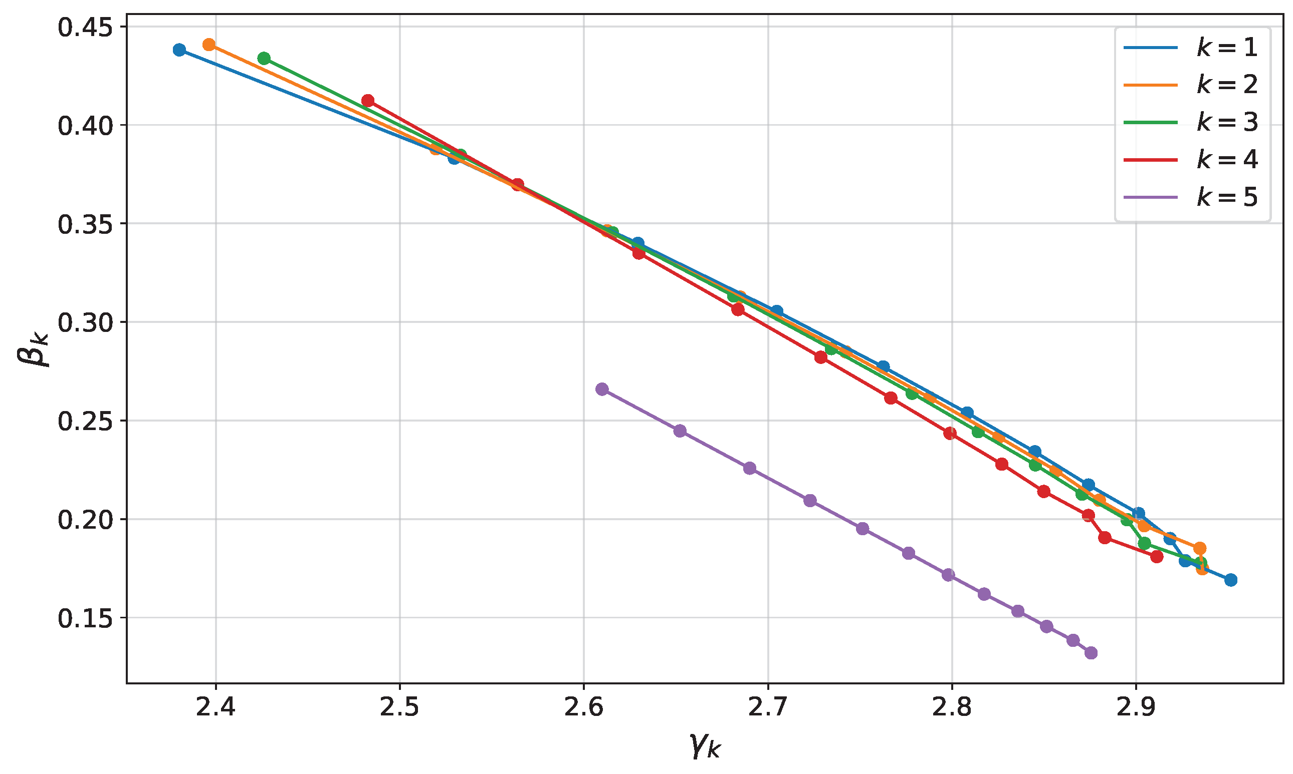
4.1. Parameter Concentration in $p\ge 2$ QAOA

From expression (3), overlaps for circuits of different depths are related recursively as

$$\begin{array}{c}\hfill g_{p+1}(\mathbf{\gamma },\mathbf{\beta },{\gamma }_{p+1},{\beta }_{p+1})=g_p(\mathbf{\gamma },\tilde{\mathbf{\beta }})+g_p(\mathbf{\gamma },\mathbf{\beta }){\cos }^n{\beta }_{p+1}(e^{-i{\gamma }_{p+1}}-1),\end{array}$$

(30)

where $\tilde{\mathbf{\beta }}=({\beta }_1+{\beta }_{p+1},\dots ,{\beta }_p+{\beta }_{p+1})$. This recursion was used in [27] for $p=2$ where it was shown that in the thermodynamic limit $n\to \infty$ the zero derivative conditions let one obtain solutions for which $n\beta \to \pi$ and $\gamma \to \pi$. This establishes parameter concentrations. The effect was further confirmed numerically on up to $n=17$ qubits and $p=5$ layers. For arbitrary depth, parameter concentrations are conjectured, yet analytical confirmation remains open. The recursion (30) can be used in the suggested operator formalism to derive a system of equations to calculate optimal parameters for circuits of arbitrary depth. In the suggested formalism the zero derivative conditions will contain expectations of propagators used in the circuit, and the system can be solved in the thermodynamic limit, albeit with a growing number of equations to satisfy.

4.2. Last Layer Behaviour

Theorem 1 establishes the linear relation between optimal parameters independent of the number of qubits n. Using a global training strategy for the same problem with $p\ge 2$ depth circuits, it was numerically observed [27] that optimal parameters depend on the depth, yet usually can be approximately described by some linear relation. In the present work, we have observed that the last layer is distinctively characterised by the very same linear relation ${\gamma }_p+2{\beta }_p=\pi$ stated in Theorem 1. We numerically confirmed this up to $p=5$ layers and $n=17$ qubits, as shown in Figure 1. The effect remains unexplained analytically and could be the manifestation of some hidden ansatz symmetry.

4.3. Saturation in Layerwise Training at $p=n$

It was demonstrated [28] that layerwise training saturates, meaning that past a critical depth $p^{\ast }$, overlap cannot be improved with further layer additions. Due to this effect, naive layerwise training performance falls below global training. Training saturation in layerwise optimisation was reported in [28] and confirmed up to $n=10$ qubits. Most surprisingly, the saturation depth $p^{\ast }$ was observed to be equal to the number of qubits n. Two effects remain unexplained analytically. Firstly does $p^{\ast }=n$. Secondly, could one go beyond the necessary conditions in [28] to explain saturations?

4.4. Removing Saturation in Layerwise Training

Any modification in the layerwise training process that violates the necessary saturation conditions can remove the system from its original saturation points. This idea was exploited in [28], where two types of variations were introduced for system sizes up to $n=7$: (i) undertraining the QAOA circuit at each iteration and (ii) training in the presence of random coherent phase noise. Whereas both modifications (i) and (ii) removed saturations at $p=n$ yet the reason remains unexplained.

5. Conclusions

We have proven a relationship between optimal QAOA parameters for $p=1$, and we recover optimal angles in the thermodynamic limit. We demonstrated the effect of parameter concentrations for $p=1$ QAOA circuits using an operator formalism. Compared to the explicit calculation where objective function gradients are set to zero, the operator approach exploits the ansatz symmetry in finding optimal parameters. The suggested approach can directly be adopted to find optimal parameters for the $p\ge 2$ QAOA circuit, with increasing complexity due to the larger number of parameters. Finally, we present a list of numerical effects, observed for particular system size and circuit depth, which are yet to be explained analytically. These unexplained effects include both limitations and advantages to QAOA. While difficult, adding missing theory to these subtle effects would improve our understanding of variational algorithms.

References

1. Harrigan, M.P.; Sung, K.J.; Neeley, M.; Satzinger, K.J.; Arute, F.; Arya, K.; Atalaya, J.; Bardin, J.C.; Barends, R.; Boixo, S.; et al. Quantum approximate optimization of non-planar graph problems on a planar superconducting processor. Nat. Phys. 2021, 17, 332–336. [Google Scholar] [CrossRef]
2. Pagano, G.; Bapat, A.; Becker, P.; Collins, K.; De, A.; Hess, P.; Kaplan, H.; Kyprianidis, A.; Tan, W.; Baldwin, C.; et al. Quantum approximate optimization of the long-range Ising model with a trapped-ion quantum simulator. arXiv 2019, arXiv:1906.02700. [Google Scholar] [CrossRef] [PubMed]
3. Guerreschi, G.G.; Matsuura, A.Y. QAOA for Max-Cut requires hundreds of qubits for quantum speed-up. Sci. Rep. 2019, 9, 6903. [Google Scholar] [CrossRef] [PubMed] [Green Version]
4. Butko, A.; Michelogiannakis, G.; Williams, S.; Iancu, C.; Donofrio, D.; Shalf, J.; Carter, J.; Siddiqi, I. Understanding quantum control processor capabilities and limitations through circuit characterization. In Proceedings of the 2020 International Conference on Rebooting Computing (ICRC), Atlanta, GA, USA, 1–3 December 2020; IEEE: Piscataway, NJ, USA, 2020; pp. 66–75. [Google Scholar]
5. Biamonte, J. Universal variational quantum computation. Phys. Rev. A 2021, 103, L030401. [Google Scholar] [CrossRef]
6. Campos, E.; Nasrallah, A.; Biamonte, J. Abrupt transitions in variational quantum circuit training. Phys. Rev. A 2021, 103, 032607. [Google Scholar] [CrossRef]
7. Farhi, E.; Goldstone, J.; Gutmann, S. A Quantum Approximate Optimization Algorithm. arXiv 2014, arXiv:1411.4028. [Google Scholar]
8. Niu, M.Y.; Lu, S.; Chuang, I.L. Optimizing qaoa: Success probability and runtime dependence on circuit depth. arXiv 2019, arXiv:1905.12134. [Google Scholar]
9. Akshay, V.; Philathong, H.; Morales, M.E.; Biamonte, J.D. Reachability Deficits in Quantum Approximate Optimization. Phys. Rev. Lett. 2020, 124, 090504. [Google Scholar] [CrossRef] [Green Version]
10. Akshay, V.; Philathong, H.; Campos, E.; Rabinovich, D.; Zacharov, I.; Zhang, X.M.; Biamonte, J. On Circuit Depth Scaling for Quantum Approximate Optimization. arXiv 2022, arXiv:2205.01698. [Google Scholar]
11. Zhou, L.; Wang, S.T.; Choi, S.; Pichler, H.; Lukin, M.D. Quantum Approximate Optimization Algorithm: Performance, Mechanism, and Implementation on Near-Term Devices. Phys. Rev. X 2020, 10, 021067. [Google Scholar] [CrossRef]
12. Brady, L.T.; Baldwin, C.L.; Bapat, A.; Kharkov, Y.; Gorshkov, A.V. Optimal Protocols in Quantum Annealing and Quantum Approximate Optimization Algorithm Problems. Phys. Rev. Lett. 2021, 126, 070505. [Google Scholar] [CrossRef] [PubMed]
13. Farhi, E.; Harrow, A.W. Quantum Supremacy through the Quantum Approximate Optimization Algorithm. arXiv 2016, arXiv:1602.07674. [Google Scholar]
14. Farhi, E.; Goldstone, J.; Gutmann, S.; Zhou, L. The quantum approximate optimization algorithm and the sherrington-kirkpatrick model at infinite size. arXiv 2019, arXiv:1910.08187. [Google Scholar] [CrossRef]
15. Wauters, M.M.; Mbeng, G.B.; Santoro, G.E. Polynomial scaling of QAOA for ground-state preparation of the fully-connected p-spin ferromagnet. arXiv 2020, arXiv:2003.07419. [Google Scholar]
16. Claes, J.; van Dam, W. Instance Independence of Single Layer Quantum Approximate Optimization Algorithm on Mixed-Spin Models at Infinite Size. arXiv 2021, arXiv:2102.12043. [Google Scholar] [CrossRef]
17. Wang, Z.; Rubin, N.C.; Dominy, J.M.; Rieffel, E.G. X Y mixers: Analytical and numerical results for the quantum alternating operator ansatz. Phys. Rev. A 2020, 101, 012320. [Google Scholar] [CrossRef] [Green Version]
18. Hodson, M.; Ruck, B.; Ong, H.; Garvin, D.; Dulman, S. Portfolio rebalancing experiments using the Quantum Alternating Operator Ansatz. arXiv 2019, arXiv:1911.05296. [Google Scholar]
19. Tsoulos, I.G.; Stavrou, V.; Mastorakis, N.E.; Tsalikakis, D. GenConstraint: A programming tool for constraint optimization problems. SoftwareX 2019, 10, 100355. [Google Scholar] [CrossRef]
20. Lloyd, S. Quantum approximate optimization is computationally universal. arXiv 2018, arXiv:1812.11075. [Google Scholar]
21. Morales, M.E.; Biamonte, J.; Zimborás, Z. On the universality of the quantum approximate optimization algorithm. Quantum Inf. Process. 2020, 19, 1–26. [Google Scholar] [CrossRef]
22. Rabinovich, D.; Adhikary, S.; Campos, E.; Akshay, V.; Anikin, E.; Sengupta, R.; Lakhmanskaya, O.; Lakhmanskiy, K.; Biamonte, J. Ion native variational ansatz for quantum approximate optimization. arXiv 2022, arXiv:2206.11908. [Google Scholar]
23. Jiang, Z.; Rieffel, E.G.; Wang, Z. Near-optimal quantum circuit for Grover’s unstructured search using a transverse field. Phys. Rev. A 2017, 95, 062317. [Google Scholar] [CrossRef] [Green Version]
24. Hastings, M.B. Classical and quantum bounded depth approximation algorithms. arXiv 2019, arXiv:1905.07047. [Google Scholar] [CrossRef]
25. Bravyi, S.; Kliesch, A.; Koenig, R.; Tang, E. Obstacles to State Preparation and Variational Optimization from Symmetry Protection. Phys. Rev. Lett. 2019, 125, 260505. [Google Scholar] [CrossRef]
26. Akshay, V.; Philathong, H.; Zacharov, I.; Biamonte, J. Reachability Deficits in Quantum Approximate Optimization of Graph Problems. Quantum 2021, 5, 532. [Google Scholar] [CrossRef]
27. Akshay, V.; Rabinovich, D.; Campos, E.; Biamonte, J. Parameter concentrations in quantum approximate optimization. Phys. Rev. A 2021, 104, L010401. [Google Scholar] [CrossRef]
28. Campos, E.; Rabinovich, D.; Akshay, V.; Biamonte, J. Training saturation in layerwise quantum approximate optimization. Phys. Rev. A 2021, 104, L030401. [Google Scholar] [CrossRef]
29. Shaydulin, R.; Wild, S.M. Exploiting symmetry reduces the cost of training QAOA. IEEE Trans. Quantum Eng. 2021, 2, 1–9. [Google Scholar] [CrossRef]
30. Streif, M.; Leib, M. Comparison of QAOA with quantum and simulated annealing. arXiv 2019, arXiv:1901.01903. [Google Scholar]
31. Skolik, A.; McClean, J.R.; Mohseni, M.; van der Smagt, P.; Leib, M. Layerwise learning for quantum neural networks. Quantum Mach. Intell. 2021, 3, 1–11. [Google Scholar] [CrossRef]
Figure 1. Optimal angles of p = 5 depth circuit for n [ 6 ; 17 ] . While the first layers can be approximately described by a linear relation, the last layer fits γ p + 2 β p = π . Moreover, the values of the last layer’s parameters are evidently distinct from the previous layers.
Mathematics 10 02601 g001
Publisher’s Note: MDPI stays neutral with regard to jurisdictional claims in published maps and institutional affiliations.