A Novel MRAC Scheme for Output Tracking

Abstract

This paper puts forward a novel output feedback model reference adaptive control (MRAC) scheme for solving an adaptive output tracking problem. The proposed control scheme only needs a scalar function to be updated online, which decreases the system adaptation complexity, compared to the existing MRAC schemes. Furthermore, the closed-loop signal boundedness and asymptotic output tracking are guaranteed with the proposed MRAC scheme. A simulation study is carried out to verify the effectiveness of the established approach.

1. Introduction

Mathematical models are essential for capturing and investigating the physical phenomena that undergo spatiotemporal evolution in most scientific and engineering applications. These models are generally obtained using the first principles of physics and fundamental physical laws. Generally, it is difficult or impossible to construct a precise mathematical model of physical plants due to various uncertainties and disturbances. As a result, how to control uncertain systems is one of the most challenging and meaningful topics.

It is well-known that robust control techniques can be employed for dynamical systems when mathematical models fail to accurately reflect physical phenomena due to the uncertainties of these systems [1,2,3]. However, such control approaches need the knowledge of characterized boundaries coming from system uncertainty parameterization, which may not be easy to determine in practice. Furthermore, in the presence of great uncertainty levels, these methods may not meet the designed system-performance requirements. On the other hand, adaptive control techniques [4,5,6] can handle high levels of uncertainty and require less modeling information compared to robust control approaches. Due to these factors, the adaptive control methodology is a viable option for numerous scientific and technical applications [7,8,9]. For example, in [7], an adaptive neuro-fuzzy system (ANFIS) was applied for grasping the force regulation of an unknown contact mechanism. For uncertain Rössler chaotic systems with unknown delays, an adaptive memoryless control scheme was developed in [9] to suppress chaotic phenomena with multiple delays and unknown uncertainties.

The model reference adaptive control (MRAC), which was originally introduced by Whitaker et al. [10,11], is a widely used adaptive control technique. The essential feature of MRAC is to develop feedback controller structures and controller parameter-updating laws to ensure the asymptotic output or state tracking of an ideal reference model system, as well as closed-loop signals boundedness, despite the system parameters uncertainties [12,13,14]. Much effort has been dedicated to the development of MRAC theory. The current results include state feedback MRAC for state tracking [15,16]; state feedback MRAC for output tracking [17,18]; and output feedback MRAC for output tracking [19,20]. When the whole state vector is difficult to obtain, output feedback MRAC for output tracking receives increasing attention. It is well-known that the adaptive controller with a standard update law [5] can make the output error dynamics between a controlled system and its reference model converge to zero asymptotically. However, its controller structure is complicated, and the computational burden is large, which may limit its applications.

In this paper, we focus on the synthesis of an output feedback MRAC for a class of dynamical systems described by a transfer function, with the system’s input and output as the only available signals. The structure of the controller is inspired by the work of Ioannou and Sun [19]. The major contributions of this work include:

• Developing a novel output feedback MRAC scheme that can guarantee asymptotic output tracking and closed-loop signal boundedness;
• Using the proposed control scheme, only a scalar function needs to be updated online, which reduces the system adaptation complexity compared to the current MRAC scheme;
• Conducting a comprehensive analysis of stability and tracking performance for the MRAC design.

The paper is organized as follows. The problem statement is formulated in Section 2. Section 3 explains the adaptive controller structure. The novel adaptive approach for updating the controller parameters is proposed in Section 4, as well as an investigation of its stability properties. In Section 5, the simulation results are reported. The work’s conclusions are found in Section 6.

2. Statement of the Problem

We consider the single-input single-output (SISO) dynamical system, which is represented by

$$\begin{array}{cc}\hfill & {\dot{x}}_p\left(t\right)=A_p{x}_p\left(t\right)+B_{p}u\left(t\right);\hfill \\ \hfill & y_p\left(t\right)=h_p^T{x}_p\left(t\right)\hfill \end{array}$$

(1)

where $u:R^{+}\to R$ is the input, and $y_p:R^{+}\to R$ is the output, and $x_p:R^{+}\to R^n$ is the n-dimensional system state vector. Let the triple $\{h_p^T,A_p,B_p\}$ be observable and controllable and have unknown elements. In the case of systems where the whole state is not accessible, only the system output is measured. The corresponding transfer function of the system is provided by

$$W_c\left(s\right)=k_c\frac{Z_c\left(s\right)}{R_c\left(s\right)}$$

(2)

where $Z_c\left(s\right)$ and $R_c\left(s\right)$ are monic polynomials of order $n-1$ and n, respectively.

The reference model is chosen as follows:

$$y_m\left(t\right)=W_m\left(s\right)\left[r\right]\left(t\right)=k_m\frac{Z_m\left(s\right)}{R_m\left(s\right)}\left[r\right]\left(t\right),$$

(3)

where $y_m\left(t\right)\in R$ is the reference model output, and $r\left(t\right)\in R$ is a uniformly bounded and piecewise-continuous reference input. $Z_m\left(s\right)$ and $R_m\left(s\right)$ are monic Hurwitz polynomials of degrees $n-1$ and n, respectively.

The objective is to determine an output feedback controller $u\left(t\right)$, so that all the system parameters and signals remain bounded, and, ideally, that the output signal $y_p\left(t\right)$ asymptotically approaches the desired reference model output $y_m\left(t\right)$ under the holding of the following assumptions:

$Assumptions$:

(1)

$Z_c\left(s\right)$ and $R_c\left(s\right)$ are coprime polynomials.

(2)

$Z_c\left(s\right)$ is Hurwitz polynomial, that is, its roots lie on the left half-plane or imaginary axis of the complex plane.

(3)

$W_m\left(s\right)$ is a strictly positive real (SPR) transfer function.

Assuming that the system output $y_p\left(t\right)$ is equal to the reference output $y_m\left(t\right)$ produces

$$y_m\left(t\right)=W_m\left(s\right)\left[r\right]\left(t\right)=W_c\left(s\right)\left[u^{*}\right]\left(t\right)=y_p\left(t\right).$$

(4)

The desired input $u^{*}\left(t\right)\in R$ is constructed as $u^{*}\left(t\right)={{\theta }^{*}}^{T}w\left(t\right)$, where ${\theta }^{*}$ is the desired controller parameter vector. On this basis, the goal of this paper is transformed into the estimation of the parameter ${\theta }^{*}$ before $y_m\left(t\right)$ is perfectly approached by $y_p\left(t\right)$. The actual controller is $u\left(t\right)={\theta }^T\left(t\right)w\left(t\right)$, where parameter vector $\theta \left(t\right)$ is the estimate of the desired controller parameter vector ${\theta }^{*}$. Details of the controller structure can be shown in the next section.

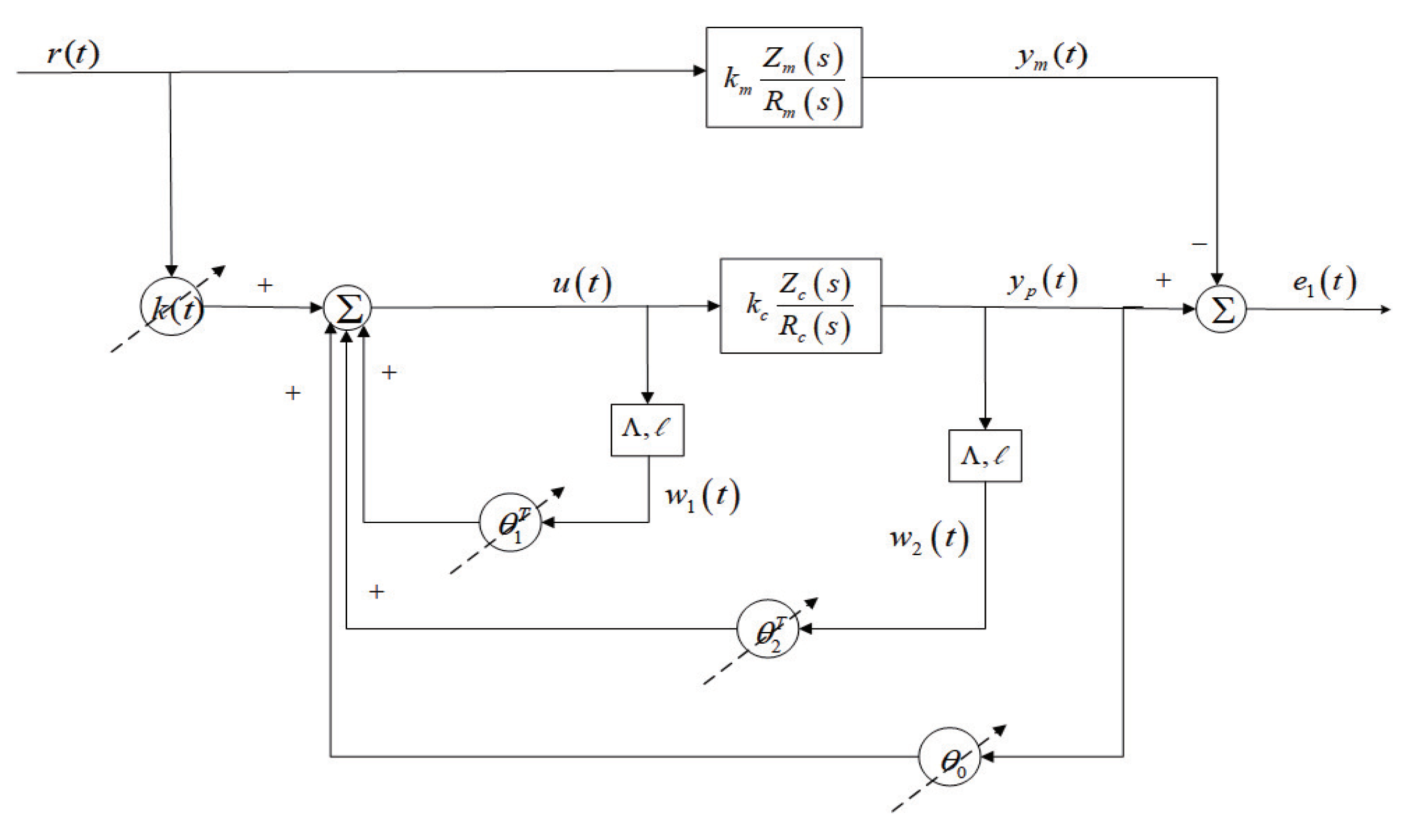
3. Controller Structure

The controller structure selected in this paper is shown in Figure 1.

The controller is described completely by the differential equation

$$\begin{array}{cc}\hfill & {\dot{w}}_1\left(t\right)=\Lambda w_1\left(t\right)+\ell u\left(t\right);\hfill \\ \hfill & {\dot{w}}_2\left(t\right)=\Lambda w_2\left(t\right)+\ell y_p\left(t\right);\hfill \\ \hfill & w{\left(t\right)}^T\triangleq [r\left(t\right),w_1^T\left(t\right),y_p\left(t\right),w_2^T\left(t\right)];\hfill \\ \hfill & \theta {\left(t\right)}^T\triangleq [k\left(t\right),{\theta }_1^T\left(t\right),{\theta }_0\left(t\right),{\theta }_2^T\left(t\right)];\hfill \\ \hfill & u\left(t\right)=\theta {\left(t\right)}^{T}w\left(t\right)\hfill \end{array}$$

(5)

where $k:R^{+}\to R,$ ${\theta }_1,w_1:R^{+}\to R^{n-1},$ ${\theta }_0:R^{+}\to R,$ ${\theta }_2,w_2:R^{+}\to R^{n-1},$ $\Lambda \in R^{(n-1)\times (n-1)}$ is an asymptotically stable matrix with $M\left(s\right)$ as its characteristic polynomial, and $(\Lambda ,\ell )$ is controllable. It follows that, when the control parameters $k\left(t\right),{\theta }_1\left(t\right),$ ${\theta }_0\left(t\right),{\theta }_2\left(t\right)$ assume constant values $k_v,{\theta }_{1v},{\theta }_{0v},{\theta }_{2v},$ respectively, the transfer functions of the feedforward and the feedback controllers are, respectively,

$$W_{1c}\left(s\right)=k_v\frac{M\left(s\right)}{M\left(s\right)-C\left(s\right)}$$

where

$$\frac{C\left(s\right)}{M\left(s\right)}\triangleq {\theta }_{1v}^T{(sI-\Lambda )}^{-1}\ell ,$$

and

$$W_{2c}\left(s\right)=\frac{D\left(s\right)}{M\left(s\right)}\triangleq {\theta }_{0v}+{\theta }_{2v}^T{(sI-\Lambda )}^{-1}\ell .$$

The overall transfer function of the system combined with the controller can be written as

$$W\left(s\right)=\frac{k_v{k}_c{Z}_c\left(s\right)M\left(s\right)}{(M\left(s\right)-C\left(s\right))R_c\left(s\right)-k_c{Z}_c\left(s\right)D\left(s\right)}$$

(6)

where $M\left(s\right)$ is a monic polynomial of degree $n-1$ and $C\left(s\right)$ and $D\left(s\right)$ are polynomials of degree $n-2$ and $n-1$, respectively. The parameter vector ${\theta }_1$ determines the coefficients of $C\left(s\right)$, while ${\theta }_0$ and ${\theta }_2$ together determine those of $D\left(s\right)$.

Let $C^{*}\left(s\right)$ and $D^{*}\left(s\right)$ be polynomials in s such that

$$M\left(s\right)-C^{*}\left(s\right)=Z_c\left(s\right),R_c\left(s\right)-k_c{D}^{*}\left(s\right)=R_m\left(s\right).$$

Further, let $M\left(s\right)=Z_m\left(s\right)$. Then scalars $k^{*},{\theta }_0^{*}$ and vectors ${\theta }_1^{*}$ and ${\theta }_2^{*}$ exist such that

$$\begin{array}{cc}\hfill & k^{*}=\frac{k_m}{k_c},\hfill \\ \hfill & {\theta }_1^{*T}{(sI-\Lambda )}^{-1}\ell =\frac{C^{*}\left(s\right)}{M\left(s\right)},\hfill \\ \hfill & {\theta }_0^{*}+{\theta }_2^{*T}{(sI-\Lambda )}^{-1}\ell =\frac{D^{*}\left(s\right)}{M\left(s\right)}.\hfill \end{array}$$

Choosing $\theta \left(t\right)\equiv {\theta }^{*}$, where the ideal controller parameter vector ${\theta }^{*}$ is defined as

$${\theta }^{*T}\triangleq [k^{*},{\theta }_1^{*T},{\theta }_0^{*},{\theta }_2^{*T}],$$

the transfer function $W\left(s\right)$ becomes

$$W\left(s\right)=k_m\frac{Z_c\left(s\right)Z_m\left(s\right)}{Z_c\left(s\right)[R_c\left(s\right)-k_c{D}^{*}\left(s\right)]}=W_m\left(s\right).$$

The differential equation describing the system together with the controller can be expressed as

$$\begin{array}{cc}\hfill & {\dot{x}}_p\left(t\right)=A_p{x}_p\left(t\right)+B_p(\theta {\left(t\right)}^{T}w\left(t\right));\hfill \\ \hfill & {\dot{w}}_1\left(t\right)=\Lambda w_1\left(t\right)+\ell (\theta {\left(t\right)}^{T}w\left(t\right));\hfill \\ \hfill & {\dot{w}}_2\left(t\right)=\Lambda w_2\left(t\right)+\ell (h_p^T{x}_p\left(t\right)).\hfill \\ \hfill \end{array}$$

(7)

In the adaptive case, we define the parameter errors as follows:

$$\begin{array}{cc}\hfill & \tilde{k}\left(t\right)\triangleq k\left(t\right)-k^{*},{\tilde{\theta }}_0\left(t\right)\triangleq {\theta }_0\left(t\right)-{\theta }_0^{*},{\tilde{\theta }}_1\left(t\right)\triangleq {\theta }_1\left(t\right)-{\theta }_1^{*},\hfill \\ \hfill & {\tilde{\theta }}_2\left(t\right)\triangleq {\theta }_2\left(t\right)-{\theta }_2^{*},\varphi {\left(t\right)}^T\triangleq [\tilde{k}\left(t\right),{\tilde{\theta }}_1^T\left(t\right),{\tilde{\theta }}_0\left(t\right),{\tilde{\theta }}_2^T\left(t\right)].\hfill \end{array}$$

Then, (7) can be rewritten as

$$\begin{array}{cc}\hfill & \dot{x}\left(t\right)=A_{c}x\left(t\right)+B_c({\varphi }^T\left(t\right)w\left(t\right)+k^{*}r\left(t\right));\hfill \\ \hfill & y_p\left(t\right)=h_c^{T}x\left(t\right)\hfill \end{array}$$

(8)

where

$$A_c=\left[\begin{array}{ccc}{A}_p+{\theta }_0^{*}{B}_p{h}_p^T& B_p{\theta }_1^{*T}& B_p{\theta }_2^{*T}\\ {\theta }_0^{*}\ell h_p^T& \Lambda +\ell {\theta }_1^{*T}& \ell {\theta }_2^{*T}\\ \ell h_p^T& 0& \Lambda \end{array}\right],$$

$$B_c=\left[\begin{array}{c}{B}_p\\ \ell \\ 0\end{array}\right];$$

$$h_c={\left[\begin{array}{ccc}{h}_p^T& 0& 0\end{array}\right]}^T,x={\left[\begin{array}{ccc}{x}_p^T& w_1^T& w_2^T\end{array}\right]}^T.$$

(9)

Since $W\left(s\right)\equiv W_m\left(s\right)$ when $\theta \left(t\right)\equiv {\theta }^{*}$, it follows that the reference model can be described by the ${(3n-2)}^{th}$ order difference equation

$$\begin{array}{cc}\hfill & {\dot{x}}_{mr}\left(t\right)=A_c{x}_{mr}\left(t\right)+B_c{k}^{*}r\left(t\right);\hfill \\ \hfill & y_m\left(t\right)=h_c^T{x}_{mr}\left(t\right)=h_p^T{x}_m\left(t\right)\hfill \end{array}$$

(10)

where

$$\begin{array}{cc}\hfill & x_{mr}={[x_m^T,w_{m1}^T,w_{m2}^T]}^T,\hfill \\ \hfill & h_c^T{(sI-A_c)}^{-1}{B}_c=\frac{k_c}{k_m}{W}_m\left(s\right).\hfill \end{array}$$

(11)

As a result, the error equation for the over system can be written as

$$\begin{array}{cc}\hfill & \dot{e}\left(t\right)=A_{c}e\left(t\right)+B_c\left[\varphi {\left(t\right)}^{T}w\left(t\right)\right];\hfill \\ \hfill & e_1\left(t\right)=h_c^{T}e\left(t\right)\hfill \end{array}$$

(12)

where $e\left(t\right)=x\left(t\right)-x_{mr}\left(t\right)$ is inaccessible and $e_1\left(t\right)=y_p\left(t\right)-y_m\left(t\right)$ corresponds to the output error. In addition, in this configuration,

$$W_e\left(s\right)=h_c^T{(sI-A_c)}^{-1}{B}_c=\frac{1}{k^{*}}{W}_m\left(s\right)$$

(13)

is a transfer function that is strictly positive real (SPR).

The standard adaptive update law [5] for the dynamical systems with the relative degree $n^{*}=1$ can be expressed as

$$\dot{\theta }\left(t\right)=-{\Gamma }_{s}w\left(t\right)e_1\left(t\right)$$

(14)

where ${\Gamma }_s={\Gamma }_s^T>0$ is a gain matrix, and $e_1\left(t\right)=y_p\left(t\right)-y_m\left(t\right)$ is the output error. The adaptive controller with standard update law (14) can make the output error dynamics between the controlled system and reference model converge to zero asymptotically. However, this controller has a large computational burden. In detail, the adaptive controller requires estimating a number of unknown updated parameters online. $\theta \left(t\right)\in R^{2n}$ is an updated parameters vector satisfying $2n$ update laws. Furthermore, the number of adaption parameters to be updated online with this classical control scheme will increase as the number of system states increases. This undoubtedly increases the computational cost and resource consumption for increasingly complex dynamic systems. Thus, reducing the number of parameters to be updated online is a significant problem for the output feedback MRAC.

4. Design and Stability Properties of the Proposed MRAC Scheme

In this section, we provide the design and stability properties of the proposed MRAC scheme.

Following the aforementioned analysis, we further explore an adaptive control scheme that reduces the number of adaptive update laws. For this purpose, we design the scalar function $\psi \left(t\right)\in R$. Accordingly, $\dot{\theta }\left(t\right)=\delta \dot{\psi }\left(t\right)$, where $\delta =\left({\delta }_i\right)\in R^{2n}$ is a design parameter vector satisfying ${\delta }_i\ne 0$ for some $i\in (1,\dots ,n).$ Now, let the parameter error have the form given by $\varphi \left(t\right)=\delta \psi \left(t\right)$ to find the scalar update law for the MRAC. The system error dynamics can, thus, be written as follows:

$$\begin{array}{cc}\hfill & \dot{e}\left(t\right)=A_{c}e\left(t\right)+B_c{\delta }^T\psi \left(t\right)w\left(t\right);\hfill \\ \hfill & e_1\left(t\right)=h_c^{T}e\left(t\right).\hfill \end{array}$$

(15)

The following theorem presents the major finding of this study.

Theorem 1.

Consider the dynamical system denoted by (1), the designed reference model denoted by (3) under the aforementioned assumptions, and the control law defined by (5). When the parameter update laws are designed as

$$\dot{\theta }\left(t\right)=\delta \dot{\psi }\left(t\right)$$

(16)

with the scalar update law

$$\dot{\psi }\left(t\right)=-\frac{e_1^T\left(t\right){\delta }^{T}w\left(t\right)}{tr({\delta }^T\Gamma \delta )},$$

(17)

where $\Gamma ={\Gamma }^T>0$, $e_1\left(t\right)=y_p\left(t\right)-y_m\left(t\right)$. Then, all closed-loop signals are bounded, and the asymptotic tracking is achieved as $\underset{t\to \infty }{lim}\mid y_p\left(t\right)-y_m\left(t\right)\mid =0.$

Proof. 

Consider the following Lyapunov function candidate, which is positive definite and decrescent

$$\begin{array}{c}V(e\left(t\right),\psi \left(t\right))=\frac{1}{2}{e}^T\left(t\right)Pe\left(t\right)+\frac{1}{2}tr[\left({\delta }^T\psi \left(t\right)\right)\Gamma \left(\delta \psi \left(t\right)\right)]\hfill \end{array}$$

(18)

where P and $\Gamma$ are a constant symmetric and positive definite matrix.

Differentiating expression (18) yields

$$\dot{V}(e\left(t\right),\psi \left(t\right))=e^T\left(t\right)P\dot{e}\left(t\right)+tr[\left({\delta }^T\psi \left(t\right)\right)\Gamma (\delta \dot{\psi }\left(t\right))].$$

(19)

Substituting expression (15) in (19) and using the properties of the transposition, we obtain

$$\begin{array}{cc}\hfill \dot{V}(e\left(t\right),\psi \left(t\right))& =\frac{1}{2}{e}^T\left(t\right)(P{A}_c+A_c^{T}P)e\left(t\right)+e^T\left(t\right)P{B}_c{\delta }^T\psi \left(t\right)w\left(t\right)+tr[\left({\delta }^T\psi \left(t\right)\right)\Gamma (\delta \dot{\psi }\left(t\right))]\hfill \\ & =\frac{1}{2}{e}^T\left(t\right)(P{A}_c+A_c^{T}P)e\left(t\right)+e^T\left(t\right)P{B}_c{\delta }^T\psi \left(t\right)w\left(t\right)+\psi \left(t\right)tr({\delta }^T\Gamma \delta )\dot{\psi }\left(t\right).\hfill \end{array}$$

(20)

Since the transfer function (13) is SPR, using the Meyer–Kalman–Yakubovich (MKY) Lemma [5], we can ensure that given a matrix $Q=Q^T>0$, there exists a $P=P^T>0$, such that

$$\left\{\begin{array}{c}P{A}_c+A_c^{T}P=-Q,\hfill \\ b_c^{T}P=h_c^T.\hfill \end{array}\right.$$

(21)

Using this fact in (21), it follows that

$$\begin{array}{cc}\hfill \dot{V}(e\left(t\right),\psi \left(t\right))& =-\frac{1}{2}{e}^T\left(t\right)Qe\left(t\right)+e^T\left(t\right)h_c{\delta }^T\psi \left(t\right)w\left(t\right)+\psi \left(t\right)tr({\delta }^T\Gamma \delta )\dot{\psi }\left(t\right)\hfill \\ & =-\frac{1}{2}{e}^T\left(t\right)Qe\left(t\right)+e_1^T\left(t\right){\delta }^T\psi \left(t\right)w\left(t\right)+\psi \left(t\right)tr({\delta }^T\Gamma \delta )\dot{\psi }\left(t\right).\hfill \end{array}$$

(22)

If we choose the scalar update law as

$$\dot{\psi }\left(t\right)=-\frac{e_1^T\left(t\right){\delta }^{T}w\left(t\right)}{tr({\delta }^T\Gamma \delta )},$$

(23)

then the derivative of the Lyapunov function (22) becomes

$$\dot{V}(e\left(t\right),\psi \left(t\right))=-\frac{1}{2}{e}^T\left(t\right)Qe\left(t\right).$$

(24)

Accordingly,

$$\dot{V}(e\left(t\right),\psi \left(t\right))\le -\frac{1}{2}{\lambda }_{min}\left(Q\right){\parallel e\left(t\right)\parallel }^2\le 0.$$

(25)

In addition, $\dot{V}(e\left(t\right),\psi \left(t\right))$ can be shown to be uniformly continuous by examing the boundedness of its derivative. Then, using Barbalat’s Lemma [21], we can deduce that $\dot{V}(e\left(t\right),\psi \left(t\right))\to 0$, and hence $e_1\left(t\right)\to 0$. Therefore, the output tracking error is asymptotically stable and closed-loop signals remain bounded. This completes the proof of Theorem 1. □

Complexity analysis. To better illustrate the computational advantage of the proposed MRAC scheme and the clarity of presentation, we, respectively, list the adaptive controllers and update laws involved as follows:

From

Table 1. The adaptive controllers and update laws in the standard MRAC and this paper.

	Adaptive Controller	The Update Law
The adaptive controller with standard update law (14)	$u\left(t\right)=\theta {\left(t\right)}^{T}w\left(t\right)$	$\dot{\theta }\left(t\right)=-{\Gamma }_{s}w\left(t\right)e_1\left(t\right)$
The adaptive controller based on the scalar update law (16)	$u\left(t\right)=\theta {\left(t\right)}^{T}w\left(t\right)$	$\dot{\theta }\left(t\right)=\delta \dot{\psi }\left(t\right)=-\delta \frac{e_1^T\left(t\right){\delta }^{T}w\left(t\right)}{tr({\delta }^T\Gamma \delta )}$

, we can see that the form of the adaptive controller we designed is the same as the standard adaptive controller; both of them are $u\left(t\right)=\theta {\left(t\right)}^{T}w\left(t\right)$. They all need to design $\theta \left(t\right)$. The difference between the calculation method in the standard adaptive controller and ours is that the standard adaptive controller needs to calculate $2n$ update laws online, $\dot{\theta }\left(t\right)=-{\Gamma }_{s}w\left(t\right)e_1\left(t\right)$, and ours only needs to calculate one, $\dot{\theta }\left(t\right)=\delta \dot{\psi }\left(t\right)=-\delta \frac{e_1^T\left(t\right){\delta }^{T}w\left(t\right)}{tr({\delta }^T\Gamma \delta )}$. Moreover, the computational complexity of each update law in the standard adaptive controller is similar to that of the scalar update law in our method. In general, the computational complexity of the adaptive controller in the standard adaptive controller is $2n$ times that of ours.

Remark 1.

To further illustrate the effectiveness of the adaptive controller based on the scalar update law (16) more briefly, we give a comparison of the number of update laws and the stability property of the output error dynamics with the adaptive controller with standard update law (14) in

Table 2. The comparison of computation and stability property.

Controller	The Number	Stability Property of the
	of Update Laws	Output Error Dynamics
The adaptive controller with standard update law (14)	$2n$	asymptotically stable
The adaptive controller based on the scalar update law (16)	1	asymptotically stable

.

Remark 2.

Similar to the study of the classical error models [5,22], we can obtain that if the signal vector $w\left(t\right)$ satisfies the persistent excitation (PE) condition [23], namely, there exist positive constants T and ${\epsilon }_0$, the following equation holds for any $t\ge t_0$

$${\int }_t^{t+T}w\left(\tau \right)w{\left(\tau \right)}^{T}d\tau \ge {\epsilon }_{0}I,$$

then the parameter error $\varphi \left(t\right)$ can converge to zero.

5. Simulation

In this section, the following adaptive control issue will be simulated to show the utility of the suggested approach.

The transfer functions of the controlled system and the reference model are selected to be

$$W_c\left(s\right)=\frac{s+1}{s^2-5s+6}$$

(26)

and

$$W_m\left(s\right)=\frac{s+2}{s^2+3s+6}$$

(27)

respectively. The fix control parameters $\Lambda$ and ℓ in (5) were chosen as $\Lambda =-2$ and $\ell =1$. In addtion, therefore, we obtain that the true values of the control parameter are ${\theta }^{*}={[1,1,-8,16]}^T$. From (14) and (16), we can obtain that the number of update laws in the adaptive controller with the method in standard MRAC and of this paper are 4 and 1, respectively.

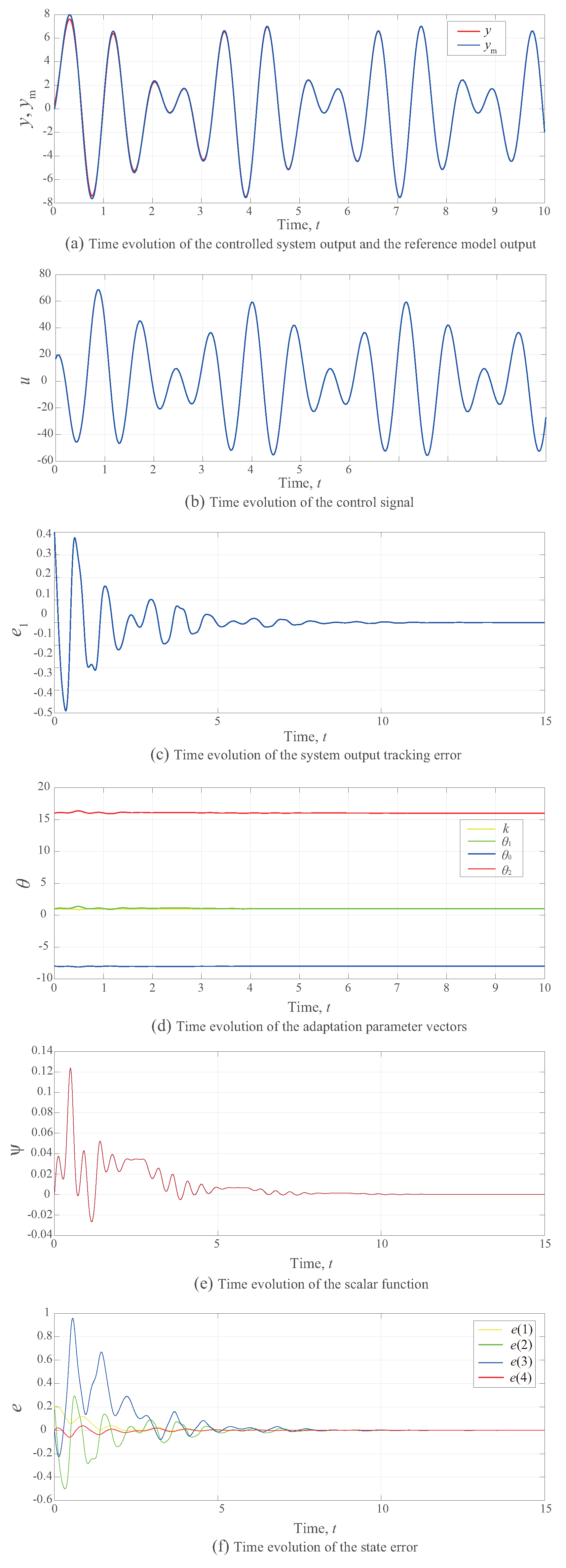
To validate the tracking effectiveness of the developed adaptive controller, we apply our proposed MRAC scheme to the adaptive parameters. For convenience, we chose $\Gamma =I_2$, $\delta ={[-1,1,3,2]}^T$, $y_p\left(0\right)={[0.2,0.2]}^T$, $y_m\left(0\right)={[0,0]}^T$; the other initial conditions were set to be zero. The simulation findings are given in Figure 2 for the case $r\left(t\right)=30\ast sin(8\ast t)+20\ast cos(6\ast t)$.

The time response of the controlled system output and the reference model output is shown in Figure 2a. We can see that the system response follows the reference trajectory rapidly.

Figure 2b presents the time evolution of the control input signal, confirming that the control signal remains within acceptable ranges. Figure 2c,d show the system output tracking error and adaptation parameter vectors, respectively, where we demonstrate the online adaptation of the controller parameter such that the tracking error convergence towards zero and closed-loop system signals are bounded. Moreover, Figure 2e,f show the time evolution of scalar function $\psi \left(t\right)$ and state error $e\left(t\right)$, respectively, illustrating the boundedness of the scalar function $\psi \left(t\right)$, and the asymptotic convergence of $e\left(t\right)$ to zero.

Furthermore, under the same condition, we compared the system output y and the output error $e_1$ with the standard MRAC. For convenience, we chose ${\Gamma }_s=I_2$ in the standard adaptive controller. Figure 3 shows the simulation findings.

From Figure 3, we can find that both the proposed MRAC scheme and the standard MRAC scheme can make the output error dynamic asymptotically stable. In addition, we can also see that the proposed controller maintains better control performance compared to the standard adaptive controller, in terms of tracking precision and rapidity.

In addition, we also compared the running times of the system with these two adaptive controllers. The running results show that it needs 0.1490 s to complete computation with the standard MRAC scheme, while in this example it only takes 0.0480 s using the proposed controller. Therefore, the method in this paper is computationally less demanding than the methods in standard MRAC. Based on the above numerical results, our control strategy can have fewer update parameters and less computational burden than the standard MRAC scheme, while maintaining the asymptotic stability of the system output error dynamics.

$Caseofinterference$:

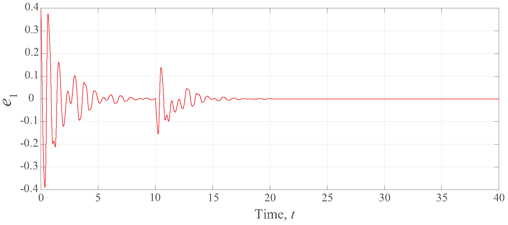
In order to make the simulation more realistic, an additive interference was inserted to the system (26) at $t=10$ s. For this case, the simulation result is shown in Figure 4. This example shows that, even in case of parametric variations, the proposed MRAC scheme maintains its performances and the asymptotic tracking of the reference model trajectory.

6. Conclusions

Due to various uncertainties, it is difficult or impossible to construct accurate mathematical models of physical plants. When the whole state vector is difficult to obtain, output feedback MRAC can deal with system uncertainty, so it has received increasing attention among researchers. However, the existing adaptive controller structure is complicated, and the computational burden is large, which may limit its applications. Therefore, in this paper, we developed a novel output feedback MRAC framework that ensures asymptotic output tracking and signal boundedness in a closed loop. Using the control scheme, only one parameter needs to be updated online, so the computational burden problem in the existing output feedback MRAC can be reduced. The adaptive control design’s closed-loop system stability and tracking performance were thoroughly analyzed. We also presented simulation results for the proposed approach, demonstrating that the required adaptive control system performance was achieved. Further work will include extensions to fractional-order model reference adaptive control (FOMRAC).

References

- Weinman, A. Uncertain Models and Robust Control; Springer: New York, NY, USA, 1991. [Google Scholar]
- Zhou, K.; Doyle, J.C.; Glover, K. Robust and Optimal Control; Prentice-Hall: Englewood Cliffs, NJ, USA, 1996. [Google Scholar]
- Dullerud, G.E.; Paganini, F. A Course in Robust Control Theory: A Convex Approach; Springer: New York, NY, USA, 2014. [Google Scholar]
- Astrom, K.J.; Wittenmark, B. Adaptive Control; Addison-Wesley: Reading, MA, USA, 1989. [Google Scholar]
- Narendra, K.S.; Annaswamy, A.M. Stable Adaptive Systems; Dover Publication Inc.: Mineola, NY, USA, 2005. [Google Scholar]
- Ortega, R.; Gerasimov, D.N.; Barabanov, N.E.; Nikiforov, V.O. Adaptive control of linear multivariable systems using dynamic regressor extension and mixing estimators: Removing the high-frequency gain assumptions. Automatica 2019, 110, 108589. [Google Scholar] [CrossRef]
- Treesatayapun, C. Adaptive control based on IF–THEN rules for grasping force regulation with unknown contact mechanism. Robot. Comput. Integr. Manuf. 2014, 30, 11–18. [Google Scholar] [CrossRef]
- Guo, J.X.; Tao, G.; Liu, Y. A multivariable MRAC scheme with application to a nonlinear aircraft model. Automatica 2011, 47, 804–812. [Google Scholar] [CrossRef]
- Yan, J.J.; Kuo, H.H. Adaptive Memoryless Sliding Mode Control of Uncertain Rössler Systems with Unknown Time Delays. Mathematics 2022, 10, 1885. [Google Scholar] [CrossRef]
- Whitaker, H.P.; Yamron, J.; Kezer, A. Design of Model Reference Control Systems for Aircraft; Instrumentation Laboratory, Massachusetts Institute of Technology: Cambridge, MA, USA, 1958. [Google Scholar]
- Osburn, P.V.; Whitaker, H.P.; Kezer, A. New Developments in the Design of Model Reference Adaptive Control Systems; Institute of Aeronautical Sciences: Traverse, MI, USA, 1961; Volume 61. [Google Scholar]
- Ristevski, S.; Dogan, K.M.; Yucelen, T. Transient Performance Improvement in Reduced Order Model Reference Adaptive Control Systems. IFAC-PapersOnLine 2019, 52, 49–54. [Google Scholar] [CrossRef]
- Nguyen, N.T. Model Reference Adaptive Control: A Primer; Springer: Belmont, CA, USA, 2018; pp. 40–41. [Google Scholar]
- Yang, J.; Na, J.; Gao, G.B. Robust model reference adaptive control for transient performance enhancement. Int. J. Robust Nonlinear Control 2020, 30, 6207–6228. [Google Scholar] [CrossRef]
- Tao, G.; Joshi, S.M.; Ma, X. Adaptive state feedback and tracking control of systems with actuator failures. IEEE Trans. Autom. Control 2001, 46, 78–95. [Google Scholar] [CrossRef]
- Anderson, R.B.; Marshall, J.A.; L’Afflitto, A. Novel model reference adaptive control laws for improved transient dynamics and guaranteed saturation constraints. J. Frankl. Inst. 2021, 358, 6281–6308. [Google Scholar] [CrossRef]
- Tao, G. Adaptive Control Design and Analysis; John Wiley Sons: Hoboken, NJ, USA, 2003. [Google Scholar]
- Song, G.; Tao, G. Partial-state feedback multivariable MRAC and reduced-order designs. Automatica 2020, 47, 804–812. [Google Scholar] [CrossRef]
- Ioannou, P.A.; Sun, J. Robust Adaptive Control; Prentice-Hall: Upper Saddle River, NJ, USA, 1996. [Google Scholar]
- Duarte-Mermoud, M.A.; Aguila-Camacho, N.; Gallegos, J.A.; Castro-Linares, R. Using general quadratic Lyapunov functions to prove Lyapunov uniform stability for fractional order systems. Commun. Nonlinear Sci. Numer. Simul. 2015, 22, 650–659. [Google Scholar] [CrossRef]
- Krstic, M.; Kanellakapoulos, I. Non Linear and Adaptive Control Design; Wiley: New York, NY, USA, 1995. [Google Scholar]
- Narendra, K.S.; Annaswamy, A.M. Persistent excitation in adaptive systems. Int. J. Control 1987, 45, 127–160. [Google Scholar] [CrossRef]
- Anderson, B.D.O.; Johnson, C.R., Jr. Exponential convergence of adaptive identification and control algorithms. Automatica 1982, 18, 1–13. [Google Scholar] [CrossRef]