Article

An Improved Reptile Search Algorithm Based on Lévy Flight and Interactive Crossover Strategy to Engineering Application

1
College of Mathematics and Computer Application, Shangluo University, Shangluo 726000, China
2
Department of Applied Mathematics, Xi’an University of Technology, Xi’an 710054, China
3
Electronic Information and Electrical Engineering College, Shangluo University, Shangluo 726000, China
*
Author to whom correspondence should be addressed.
Mathematics 2022, 10(13), 2329; https://doi.org/10.3390/math10132329
Submission received: 29 May 2022 / Revised: 21 June 2022 / Accepted: 30 June 2022 / Published: 3 July 2022
(This article belongs to the Special Issue Optimisation Algorithms and Their Applications)

Abstract

:
In this paper, we propose a reptile search algorithm based on Lévy flight and interactive crossover strategy (LICRSA), and the improved algorithm is employed to improve the problems of poor convergence accuracy and slow iteration speed of the reptile search algorithm. First, the proposed algorithm increases the variety and flexibility of the people by introducing the Lévy flight strategy to prevent premature convergence and improve the robustness of the population. Secondly, an iteration-based interactive crossover strategy is proposed, inspired by the crossover operator and the difference operator. This strategy is applied to the reptile search algorithm (RSA), and the convergence accuracy of the algorithm is significantly improved. Finally, the improved algorithm is extensively tested using 2 test sets: 23 benchmark test functions and 10 CEC2020 functions, and 5 complex mechanical engineering optimization problems. The numerical results show that LICRSA outperforms RSA in 15 (65%) and 10 (100%) of the 2 test sets, respectively. In addition, LICRSA performs best in 10 (43%) and 4 (40%) among all algorithms. Meanwhile, the enhanced algorithm shows superiority and stability in handling engineering optimization.

1. Introduction

Almost all scientific and engineering fields can readily translate into optimization problems [1,2,3], given the different real-world requirements of various application domains [4]. These optimization problems often include many needs and requirements, such as uncertainty, multi-objective, and high dimensions, whereas finding a solution strategy for optimization problems is usually a specification [5]. In contrast, various complex issues emerge as the different domains are deepened. Therefore, a more robust and faster solution is needed to solve them. This trend suggests that scientists need to find an algorithm adaptable to various applications to meet the complex situations of difficult problems in cutting-edge engineering fields [6,7]. A wide variety of optimization algorithms are found in delving into the literature on the proposed optimization algorithms [8,9]. These evolved from traditional optimization techniques using planning techniques to nature-inspired metaheuristic algorithms, each with its highlights [10,11]. As a general-purpose optimization method, traditional algorithms often fail to provide solutions that can solve the problem when faced with optimization problems of high complexity and high gradient variability in high dimensions [12,13]. In contrast, the MH benefits from multi-group cooperation through shared experience to find the optimal solution accurately, bypassing the optimal local solution. It has the advantages of being easy to understand, converging quickly, and avoiding getting trapped in a local optimum [14,15,16].
In the latest decade, many MH algorithms have been proposed. In general, there is no standard/unique classification of metaheuristic algorithms. In this research, MH algorithms can be classified into four categories based on the source of inspiration: population intelligence (SI)-based, human-based algorithms, physics/chemistry-based algorithms, and evolutionary algorithms.
SI methods are usually inspired by the real-life and cooperative behaviors of different plants and animals in nature, and these methods search for the optimal solution adaptively by exchanging and sharing the information flow of multiple candidate solutions. Also, this approach is the most extended. Methods of this type include but are not limited to krill herd (KH) [17], GOA [18], moth flame optimization algorithm (MFO) [19], gray wolf optimizer (GWO) [20], red fox optimization algorithm (RFO) [21], slime mould algorithm (SMA) [22], aquila optimizer (AO) [23], Harris hawks optimization (HHO) [8], whale optimization algorithm (WOA) [24], sparrow search algorithm (SSA) [25], and butterfly optimization algorithm (BOA) [26].
Genetic laws often influence evolutionary algorithms, mimicking the crossover and variation behavior therein. Methods of this type include, but are not limited to, evolutionary strategy (ES) [27], genetic algorithm (GA) [28].
Physics-based and chemistry-based methods mimic physical theorems or chemical phenomena prevalent in the universe and life, usually based on universal rules to distinguish the interactions between candidate solutions. There are various methods in this class, such as atomic search optimization (ASO) [29], thermal exchange optimization (TEO) [30], multi-verse optimization algorithm (MVO) [31], chemical reaction optimization (CRO) [32], and gravity search algorithms (GSA) [33].
The final method classified in this research is a human-based algorithm, mainly motivated by social and natural behavior and guided by autonomous human thought. This method contains human mental search (HMS) [34], student psychology based-optimization algorithm (SPBO) [35], and TLBO [36].
SI-based method, as a subset of the MH algorithm, has some more significant advantages: (1) More frequent information exchange. (2) The structure of the algorithm is more straightforward. (3) It is less prone to fall into local optimal solutions. Therefore, SI-based methods have been applied to deal with complex sequential optimization issues such as feature selection [37] and surface shape parameter optimization [12,38]. However, many methods in SI are not powerful enough and often cannot handle optimization situations with a wide range of scope areas, which may be due to the low level of development and exploration and poor diversity of some methods [39]. However, the balance between exploration and development for an SI method is an area that requires too much attention. With the increasing demands of optimization problems, many studies have proposed search strategies to ensure that balance [40,41,42]. Recently, Abualigah et al. established a proposed search algorithm—reptile search algorithm—which is capable of selecting both local and global searches to solve complex optimization problems [7]. The method mainly simulates the encirclement mechanism in the exploration stage and the hunting mechanism in the exploitation stage of the crocodile.
However, some experimental results also demonstrate that RSA also has the problem of poor convergence and slow convergence when facing high-dimensional complex nonlinear optimization problems. Therefore, this paper uses some promising modification strategies to enhance the RSA algorithm capability. Firstly, Lévy flight has been considered an excellent strategy to help optimization algorithms improve their performance [43]. Zhang et al. applied the Lévy flight strategy to the backtracking search algorithm to solve the parameter estimation of the PV model [44]. OB-LF-ALO is an efficient algorithm optimized by Lévy flight and is employed to deal with some specific mechanical optimization in life [45]. Feng et al. proposed a Lévy flight-based gravitational search algorithm for solving ecological scheduling of step hydro power plants [46]. Further, Gao et al. suggested an enhanced chicken flock algorithm based on Lévy flight for the multi-objective optimization problem of integrated energy for smart communities, considering the utility of decision-makers [47]. Therefore, the Lévy flight strategy is introduced into the reptile search algorithm in this paper to improve the global search capability of RSA and guarantee the search to escape the local optimum. Moreover, influenced by the crossover operator [48] and the difference operator [49], an interactive crossover strategy is proposed in this paper. In this strategy, the candidate solutions are more influenced by the iterative process, making the difference between the preliminary search and the later development more obvious. Therefore, an improved reptile search algorithm (LICRSA) based on Lévy flight and interactive crossover is proposed in this study based on these two strategies.
The remainder of this paper is structured as follows: Section 2 presents a comprehensive description of the reptile search algorithm. Section 3 depicts the contents of both Lévy flight and crossover strategies. In Section 4, the algorithm is evaluated using 23 benchmark functions and CEC2020 and compared with different MH methods. Section 5 selects five commonly used mechanical engineering optimization problems the proposed algorithm solves. Section 6 summarizes the work.

2. Description of the Reptile Search Algorithm (RSA)

The reptile search algorithm mainly imitates the predation strategy and social behavior of crocodiles in nature [7]. The first is the encirclement mechanism in the exploration phase, and the second is the hunting mechanism in the exploitation phase. A standard MH algorithm tends to be first applied to a set of candidate solutions before the iteration starts. It is a random strategy generated.
Z = z 1 , 1 z 1 , j z 1 , d 1 z 1 , d z 2 , 1 z 2 , j z 2 , d z N 1 , 1 z N 1 , j z N 1 , d z N , 1 z N , j z N , d 1 z N , d
where zi,j represents the jth dimension of the ith crocodile. N is all the crocodiles, and d denotes dimension. Z is N candidate solutions randomly generated by Equation (2).
Z i , j = r a n d × ( u p l o w ) + l o w ,
where rand is a stochastic number; up and low are the maximum and minimum limits of the optimization problem.
Encircling behavior is the hallmark of the globalized search of RSA. The process is divided into two behaviors, aerial and abdominal walk. These two actions often do not allow crocodiles to get close to food. However, the crocodile will find the general area of the target food by chance after several search attempts because it is a global search of the whole solved spatial range. Meanwhile, ensure that the stage can be continuously adapted to the next developmental stage. The process is often limited to the first half of the total iteration. Equation (3) simulates the encircling behavior of the crocodile and is shown below.
z i , j ( t + 1 ) = b e s t j ( t ) × ( η i , j ( t ) ) × β R i , j ( t ) × r ,     t T M a x 4 b e s t j ( t ) × z r 1 , j × E S ( t ) × r ,     T M a x 4 t < 2 × T M a x 4
where besti,j (t) is the best-positioned crocodile at t iterations, and r is a stochastic number of 0 to 1. TMax represents the maximum iteration. ηi,j is the operator of the ith crocodile at the jth dimension and is given by Equation (4). β is a sensitive parameter controlling the search accuracy and is given as 0.1 in the original text [7]. Ri,j is the reduce function, and the equation is used to decrease the explored area and is computed by Equation (5). r1 is a stochastic integer between 1 and N, and zr1,j is the jth dimension of the crocodile at position r1. ES(t) is an arbitrary decreasing probability ratio between 2 and −2 and is given in Equation (6).
η i , j = b e s t i , j ( t ) × P i , j ,
R i , j = b e s t j ( t ) x r 2 , j b e s t j ( t ) + ε ,
E S ( t ) = 2 × r 3 × ( 1 1 T ) ,
where r2 is a random integer between 1 and N, and r3 is an integer number of −1 to 1. ε is a small value. Pi,j represents the percentage difference between the crocodile in the best position and crocodiles in the current position, updated as in Equation (7).
P i , j = α + z i , j M ( z i ) b e s t j ( t ) × ( u p j l o w j ) + ε ,
where M (zi) is the average position of the crocodile of zi and is given in Equation (8), upj and lowj are the maximum and minimum limits of the jth dimension. α is the same as β as a sensitive parameter to control the search accuracy. It was set to 0.1 in the original paper [7].
M ( z i ) = 1 n j = 1 n z i , j ,
Connected to the search process of RSA is the hunting process of local symbolic exploitation, which has two strategies in this part: coordination and cooperation. After the influence of the encirclement mechanism, the crocodiles almost lock the location of the target prey, and the hunting strategy of the crocodiles will make it easier for them to approach the target. The development phase will often find the near-optimal candidate solution after several iterations. The mathematical model of its simulated crocodile hunting behavior is presented in Equation (9). This development hunting strategy occurs in the second half of the iterations.
z i , j ( t + 1 ) = b e s t j ( t ) × P i , j ( t ) × r ,   2 × T M a x 4   t < 3 × T M a x 4   b e s t j ( t ) η i , j ( t ) × ε R i , j ( t ) × r , 3 × T M a x 4 t < 4 × T M a x 4
where bestj is the optimal position of the crocodile, ηi,j is the operator of the ith crocodile at the jth dimension and is given by Equation (4). Ri,j is the reduce function, and the equation is used to decrease the explored area and is computed by Equation (5). Algorithm 1 is the pseudo-code for RSA.
Algorithm 1: The framework of the RSA
1: Input: The parameters of RSA including the sensitive parameter α, β, crocodile size (N), and the maximum generation TMax.
2: Initializing n crocodile, zi and calculate fi.
3: Determine the best crocodile bestj.
4: while (ttMax) do
5:  Update the ES by Equation (6).
6:  for i = 1 to N do
7:   for i = 1 to N do
8:    Calculate the η, R, P by Equations (4), (5) and (7).
9:    if tTMax/4 then
10:      zi,j (t + 1) = bestj (t) × −ηi,j × βRi,j (t) × r.
11:     else if TMax/4 ≤ t < 2 * TMax/4
12:      zi,j (t + 1) = bestj (t) × zi,j × ES (t) × r.
13:     else if 2*TMax/4 ≤ t < 3*TMax/4
14:      zi,j (t + 1) = bestj (t) × Pi,j (t) × r.
15:     else
16:      zi,j (t + 1) = bestj (t) −ηi,j × εRi,j (t) × r.
17:     end if
18:    end for
19:   end for
20:   Find the best crocodile.
21:   t = t + 1.
22: end while
23: Output: The best crocodile.

3. The Proposed Hybrid RSA (LICRSA)

In this paper, the Lévy flight strategy and the interaction crossover strategy are chosen, respectively. The Lévy flight strategy helps candidate solutions leap out of local solutions and enhances the algorithm’s precision. An interaction crossover strategy mainly enhances the ability of algorithm development. The two methods are introduced primarily in the following.

3.1. Lévy Flight Strategy

The Lévy flight strategy is used in this paper to generate a random number with a replacement rand with the following characteristics: (1) The random numbers generated are occasionally large but mostly interspersed with small numbers in between. (2) The probability density function of the steps is heavy-tailed. This random number will help update the position to produce oscillations, perform a small search in the neighborhood by the fluctuations of the random number at one iteration, and help the candidate solution leap out of the local optimum.
The definition of Lévy distribution is given by Equation (10) below.
L e v y ( γ ) ~ u = t 1 γ ,   0 < γ 2 ,
The step length of the Lévy flight can be calculated as in Equation (11).
s = U | V | 1 / γ ,
where, both U and V follow Gaussian distribution as shown in Equation (12).
U ~ N ( 0 , σ U 2 ) ,   V ~ N ( 0 , σ V 2 )
where σU and σV meet the following Equations (13) and (14).
σ U = Γ ( 1 + β ) · sin ( π · β / 2 ) Γ ( ( 1 + β / 2 ) · β · 2 ( β 1 ) / 2 ) 1 / β ,
σ V = 1 ,
where Γ is a standard Gamma function and β is a parameter with a fixed 1.5.
Lévy flight strategy is deployed for the crocodile’s high and belly walking in the encircling mechanism to expand the surrounding search area effectively. Meanwhile, the Lévy flight strategy is also deployed for hunting coordination and cooperation in the hunting behavior phase to increase the flexibility of the optimal exploitation phase. The encircling mechanism based on Lévy flight is displayed in Equation (15). λ is a parameter with a fixed 0.1.
z i , j ( t + 1 ) = b e s t j ( t ) × ( η i , j ( t ) ) × β R i , j ( t ) × λ × L e v y ( γ ) ,     t T M a x 4   b e s t j ( t ) × z r 1 , j × E S ( t ) × λ × L e v y ( γ ) ,     T M a x 4 t < 2 × T M a x 4
The hunting behavior (hunting coordination and cooperation) based on Lévy flight is displayed in Equation (16).
z i , j ( t + 1 ) = b e s t j ( t ) × P i , j ( t ) × λ × L e v y ( γ ) ,   2 × T M a x 4   t < 3 × T M a x 4   b e s t j ( t ) η i , j ( t ) × ε R i , j ( t ) × λ × L e v y ( γ ) , 3 × T M a x 4 t < 4 × T M a x 4

3.2. Interaction Crossover Strategy

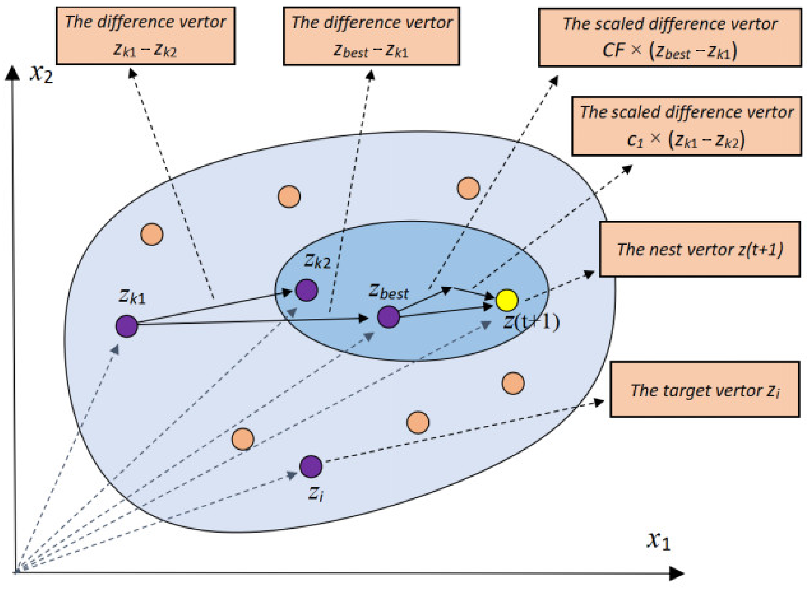
The interaction crossover strategy helps the candidate in the current position readjust by exchanging the information of the two candidate solutions and the candidate at the optimal position. The new position draws the information on the optimal solution and other candidate solutions to improve the searchability of the candidate solutions. First, a parameter controlling the activity of the crocodile population is defined, which has a linearly decreasing trend with the number of iterations. CF is defined as follows:
C F = 1 t T M a x 2 × t T M a x ,
where t represents the current iteration, TMax stands for all iterations. The crocodile population is randomly divided into two parts with the same number of crocodiles. Two positions of crocodiles zk1 and zk2 are selected from these two parts, and then the positions are interacted with to update the two crocodiles. The updated strategy is the same as that provided by Equations (18) and (19).
z k 1 , j ( t + 1 ) = z k 1 , j ( t ) + C F × ( b e s t j ( t ) z k 1 , j ( t ) ) + c 1 × ( z k 1 , j ( t ) z k 2 , j ( t ) ) ,
z k 2 , j ( t + 1 ) = z k 2 , j ( t ) + C F × ( b e s t j ( t ) z k 2 , j ( t ) ) + c 2 × ( z k 2 , j ( t ) z k 1 , j ( t ) ) ,
where bestj is the best positioned crocodile, c1 and c2 are stochastic numbers in the interval 0 to 1, and zk1 is the crocodile in position k1. Figure 1 illustrates the introduction graph of the interaction crossover.
For positions of the updated crocodiles, this paper set up an elimination mechanism: retaining the crocodiles with better positions after the interactive crossover and eliminating the crocodiles with poorer abilities. The updates are as follows:
z i , j ( t + 1 ) = z i , j ( t ) ,           i f   f ( z i , j ( t ) ) < f ( z i , j ( t + 1 ) )     z i , j ( t + 1 ) ,     e l s e i f   f ( z i , j ( t + 1 ) ) < f ( z i , j ( t ) )

3.3. Specific Implementation Steps of LICRSA

The Lévy flight strategy and the interactive crossover strategy are incorporated in RSA. These strategies effectively improve the accuracy and exploitation of the RSA algorithm while obtaining a better traversal of the cluster. The specific operation steps of LICRSA are displayed below.
Step1: Provide all the relevant parameters of LICRSA, such as the number of alligators N, the dimension of variables Dim, the upper limit up of all variables, the lower limit low of all variables, all iterations TMax, and the sensitive parameter β.
Step2: Initialize N random populations and calculate the corresponding adaptation values. The best crocodile individuals are selected.
Step3: Update ES values by Equation (6) and calculate η, R, and P values, respectively.
Step4: While t < Miter, the search phase of RSA: If t < TMax/4, update the new situation of the crocodile by the first part of Equation (15), and similarly, if t is between TMax/4 and 2TMax/4, then update the crocodile position according to the second part of Equation (15).
Step5: The development phase of RSA: if t is between 2TMax/4 and 3TMax/4, the position of the crocodile is updated by the first part of Equation (16), and in the final stage of the iteration, when t > 3TMax/4, the position of the crocodile is updated by the second part of Equation (16).
Step6: The fitness of the crocodile positions is re-evaluated, and the crocodiles with function values worse than the last iteration are eliminated, while the position of the optimal crocodile is updated.
Step7: Interactive crossover strategy: firstly, the crocodile population is divided into two parts, and then crocodiles are randomly selected from the two groups in turn for crossover, and their information is interacted by the positions of the two crocodiles updated by Equations (18) and (19), respectively.
Step8: According to the principle of Equation (20), crocodile individuals with poor predation ability are eliminated, and the optimal ones are renewed.
Step9: Determine if the iteration limit is exceeded and output the optimal value.
To show the hybrid RSA algorithm more clearly, in this paper, the pseudo-code of LICRSA is provided in Algorithm 2. Where line 10, line 12, line 14, and line 16 are the encirclement and predation phases of the Lévy flight strategy improvement. Lines 20–26 are the strategies for the interaction crossover. Figure 2 shows the flow chart of the LICRSA algorithm.
Algorithm 2: The framework of the LICRSA
1: Input: The parameters of LICRSA including the sensitive parameter α, β, crocodile size (N), the maximum generation TMax, and variable range ub, lb.
2: Initializing n crocodile, zi (i = 1, 2, …, N) and calculate the fitness fi.
3: Determine the best crocodile bestj.
4: while (ttMax) do
5:  Update the ES by Equation (6).
6:  for i = 1 to N do
7:   for i = 1 to N do
8:    Calculate the η, R, P by Equations (4), (5) and (7).
9:    if tTMax/4 then
10:      zi,j (t + 1) = bestj (t) × −ηi,j × βRi,j (t) × λ × levy(γ).
11:     else if TMax/4 ≤ t < 2 * TMax/4
12:      zi,j (t + 1) = bestj (t) × zi,j × ES (t) × λ × levy(γ).
13:     else if 2*TMax/4 ≤ t < 3*TMax/4
14:      zi,j (t + 1) = bestj (t) × Pi,j (t) × λ × levy(γ).
15:     else
16:      zi,j (t + 1) = bestj (t) −ηi,j × εRi,j (t) × λ × levy(γ).
17:     end if
18:    end for
19:   end for
20:   Update the fitness and location of the crocodile.
21:   Replace the optimal location and optimal fitness.
22:   Group = permutate(n).
23:   for i = 1 to N/2 do
24:    let k1 = Group(2 × i − 1) and k2 = Group(2 × i).
25:    Update the CF by Equation (17).
26:    zk1,j (t + 1) = zk1,j (t) + CF × (bestj(t) − zk1,j (t)) + c1 × (zk1,j (t) − zk2,j (t))
27:    zk1,j (t + 1) = zk1,j (t) + CF × (bestj(t) − zk1,j (t)) + c1 × (zk1,j (t) − zk2,j (t))
28:   end for
29:   Find the best crocodile.
30:   t = t + 1.
31: end while
32: Output: The best crocodile.

3.4. Considering the Time Complexity of LICRSA

The estimation of LICRSA time complexity is mainly based on RSA with the addition of the interaction crossover part, and the Lévy strategy only improves the update strategy of RSA. The time complexity of RSA is:
O (TMax × d × N) + O (TMax × N)
The adaptation value evaluation mainly depends on the complexity of the problem, so it is not considered in this paper. In the crossover phase, the method is a two-part population operation process, so the time complexity is:
O (TMax × d × N) + O (TMax × N) + O (TMax × d × N/2)
where d is the variables, N is all the crocodiles, and TMax is the maximum generation.

4. Simulation Experiments

To demonstrate the effectiveness of this improvement plan, 23 standard benchmark functions and CEC2020 will be used to test the local exploitation capability of LICRSA, global search capability, and ability to step out of local optimization. The experimental parameters of this section are set: the crocodile size N = 30 and the maximum iterations TMax = 1000. In addition, for each test function, all methods will be run 30 times independently in the same dimension, and the numerical results will be counted. The comparative MH algorithms in this section include reptile search algorithm (RSA) [7], aquila optimizer (AO) [23], arithmetic optimization algorithm (AOA) [4], differential evolution (DE) [49], crisscross optimization algorithm (CSO) [48], dwarf mongoose optimization (DMO) [6], white shark optimizer (WSO) [50], whale optimization algorithm (WOA) [24], wild horse optimizer (WHOA) [15], seagull optimization algorithm (SOA) [51], and gravitational search algorithm (GSA) [33] in 23 test functions. Additionally, reptile search algorithm (RSA) [7], aquila optimizer (AO) [23], arithmetic optimization algorithm (AOA) [4], differential evolution (DE) [49], dwarf mongoose optimization (DMO) [6], grasshopper optimization algorithm (GOA) [18], gravitational search algorithm (GSA) [33], honey badger algorithm (HBA) [52], HHO [8], SSA [11], and WOA [24] in CEC2020. It is worth noting that to guarantee the equity of the experiments, the parameter settings of all MH methods are the same as those provided in Table 1 and are consistent with the source paper.

4.1. Exploration–Exploitation Analysis

The two main parts of different MH algorithms are the exploration and exploitation phases. The role of exploration is that distant regions of the search domain can be explored, ensuring better search candidate solutions. Alternatively, exploitation is the convergence to the region where the optimal solution is promising and expected to be found through a local convergence strategy. Maintaining a balance between these two conflicting phases is critical for the optimization algorithm to locate the optimal candidate solution to the optimization problem [53]. Dimensional diversity in the search procedure can be expressed in Equations (23) and (24).
D i v j = 1 N i = 1 N m e d i a n ( z j ) z i , j ,
D i v ( t ) = 1 d j = 1 d D i v j , t = 1 , 2 , T M a x
where zi,j is the position of the ith crocodile in the jth dim, Divj is the average diversity of dimension j, and median(zj) is the median value of the jth dim of the candidate solution. N is all the crocodiles, d is the dim, and TMax is the maximum iteration. The following equation calculates the percentage of exploration and exploitation.
E x p l o r a t i o n % = D i v ( t ) max ( D i v ) × 100 % ,
E x p l o i t a t i o n % = D i v ( t ) max ( D i v ) max ( D i v ) × 100 % ,
where max(Div) is the maximum diversity of the iterative process.
The test set of CEC2020 is selected in this section, and Figure 3 demonstrates the exploration and exploitation behavior of LICRSA in the CEC2020 test set [5] during the search process. Analyzing Figure 3, LICRSA mainly starts from high exploration and low exploitation. Still, as the exploration proceeds, LICRSA quickly switches to high exploitation and converges to the region where the optimal solution is expected to be found. There is a partial addition of the exploration process during the iteration process, which is energetic in both exploration and utilization. Therefore, LICRSA can find better optimal solutions than other MH algorithms. In addition, Figure 4 shows the percentage of different functions, the rate of exploration is generally between 10% and 30%, which indicates that LICRSA provides enough exploration time. The rest of the effort is consumed in development. This result means that LICRSA maintains a sufficiently high exploration percentage. On the other hand, LICRSA development utilization is high.

4.2. Performance Evaluation for the 23 Classical Functions

The 23 benchmark functions include 7 unimodal, 6 multimodal, and 10 fixed-dimensional functions [5]. Among them, unimodal functions are used to explore MH algorithms, and multimodal functions are often used to understand the development of algorithms. The dimension function aims to know how well different exploration algorithms leap out of the local optimum and how accurately algorithms converge. It should be noted that the objective of all 23 functions is to minimize the problem. In addition, four criteria are used in this part of the experiment, including maximum, minimum, mean, and standard deviation (Std). In addition, the Wilcoxon signed-rank test (significance level = 0.05) is used to test for the numerical cases. Where “+” means that an algorithm is more accurate than LICRSA, “=” indicates that there is no significant difference between the two, and “−” indicates that an algorithm is less accurate than LICRSA. We also provide the p-values as reference data.
Table 2 provides the numerical case of 12 MH algorithms in solving 23 benchmark problems, where the bold indicates the most available mean and standard deviation of all algorithms. From the table, LICRSA ranked first with an average of 3.8696, and LICRSA ranked first in 10 of these test problems and second or higher in 13. The LICRSA algorithm performs the best in single-peak, ranking second or higher in 6 out of 7 unimodal functions. Meanwhile, LICRSA also performed well in multimodal functions, obtaining optimal solutions in 4 of the 6 functions (F9, F10, F11, F13). In addition, AO ranked first in 5, outperforming other MH algorithms on F5, F11, and F21, second only to LICRSA. In addition, GSA showed dominance in the fixed dimension, achieving the best runs on F16, F17, F19, F20, F22, and F23. The results show that LICRSA has more robust solution accuracy than other existing algorithms in unimodal and multimodal functions when solving the 23 benchmark problems, indicating that LICRSA can obtain a greater chance of convergence success to the optimal value resulting in good development performance. It performs better than most search algorithms in the fixed dimension. Figure 5 provides a bar plot of the mean rank of different algorithms.
In this section, the convergence analysis of the search algorithm is performed on 23 benchmark test suites. Figure 6 provides the number of functions better than LICRSA, significantly the same as LICRSA, and worse than LICRSA. 
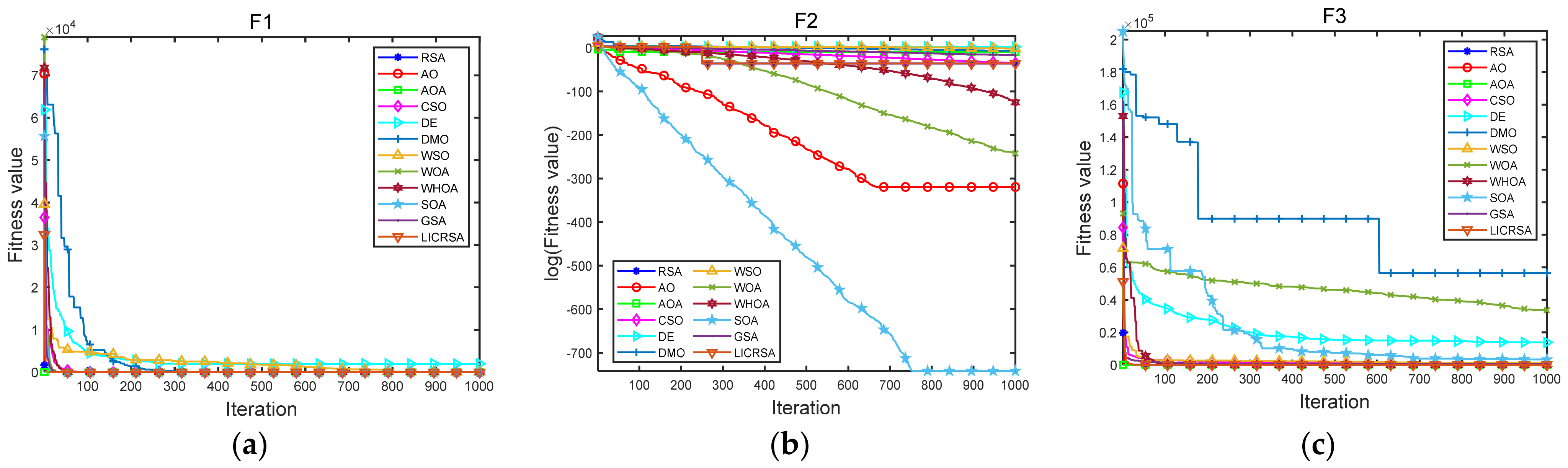
Figure 7 shows the results of the problems for the 23 test problems. Some of these functions have images for which we have taken logarithmic data processing. From the results in the figure, it can be noticed that LICRSA starts with a fast convergence and mutation behavior on most of the problems, which is more pronounced than the other tested algorithms. This result is due to the excellent exploration capability of the added interaction crossover strategy. Moreover, the results display that LICRSA has the fastest convergence on most functions than AO, AOA, RSA, CSO, DE, GSA, WOA, WHOA, DMO, SOA, and WSO. This result is due to the reduced search space and enhanced exploitation capability at iteration time by Lévy flight and crossover strategies. Also, from the convergence curves, LICRSA converges quickly to the global optimum for most unimodal and multimodal functions (F1, F3, F5, F9, F10, F11), indicating that LICRSA has better convergence capability. The results further verify the effectiveness of the Lévy flight and the interaction crossover strategy, which enhances the local search capability. In addition, Figure 8 provides the box plots of the 23 test functions, from which it is clear that the box of LICRSA is narrower, which also indicates the stability ability of LICRSA for multiple runs, and then LICRSA has some instability in the face certain fixed dimensional test functions.
Table 3 provides the final results of p-values and statistics between each algorithm and LICRSA. 1/11/11, 6/6/11, 0/6/17, 5/1/17, 1/6/16, 3/6/14 for RSA, AO, AOA, CSO, DE, and DMO, respectively, and 7/4/12, 7/4/12, 7/7/13, 7/7/13, and 7/7/13 for WSO, WOA, WHOA, SOA, and GSA. 3/7/13, 7/8/8, 1/6/16, 5/6/12.

4.3. Performance Evaluation for the CEC-2020 Test Functions

These 10 CEC2020 include a multi-peak function, 3 BASIC functions, 3 hybrid functions, and 3 composite functions [5]. The multimodal functions are usually employed to understand the development of the search algorithm, and hybrid functions can better combine the properties of sub-functions and maintain the continuity of global/local optima. The composite function combines various hybrid functions and can be employed to evaluate the convergence accuracy of the algorithm. Note that the objective of all 10 CEC2020 functions is also the minimization problem, and again, this section still uses the maximum, minimum, average, and standard deviation (Std) in the results of the numerical experiments. In addition, time metrics and p-values are also important factors in the evaluation system. In addition, the Wilcoxon signed-rank test (significance level = 0.05) is used to test the numerical cases; where “+” indicates that an algorithm is more accurate than LICRSA, “=” means that LICRSA is not different from MH, and “−” shows that a method is less accurate than LICRSA.
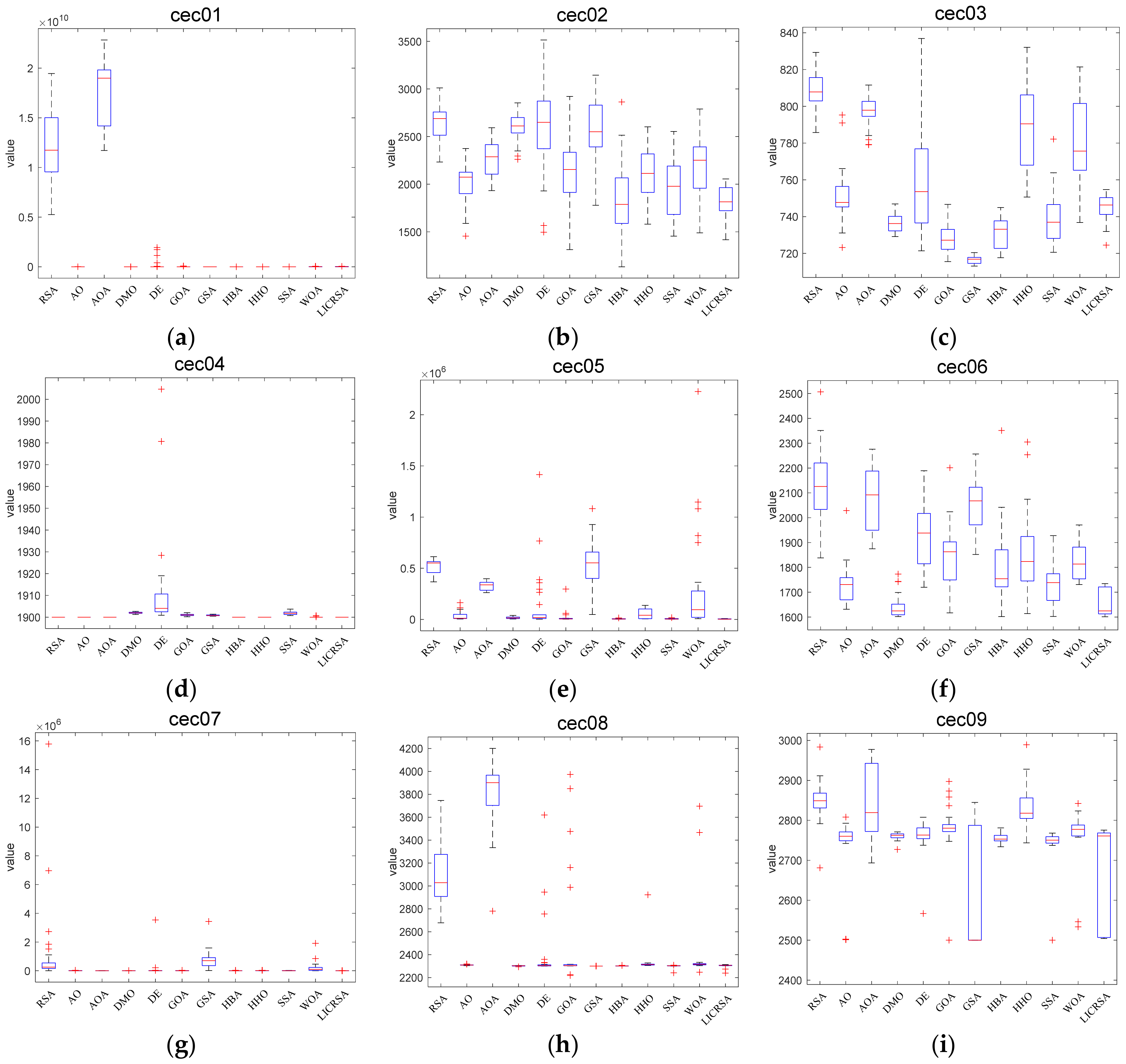
Table 4 provides a comparison between LICRSA and different MH algorithms. The table indicates that LICRSA has the best running results in four test functions, cec02, cec04, cec05, cec10, and the second ranking in cec06, cec07, and cec09, achieving the second-ranking. The overall average order of LICRSA of 2.9 is better than the other MH algorithms, indicating that LICRSA can handle this test function well.
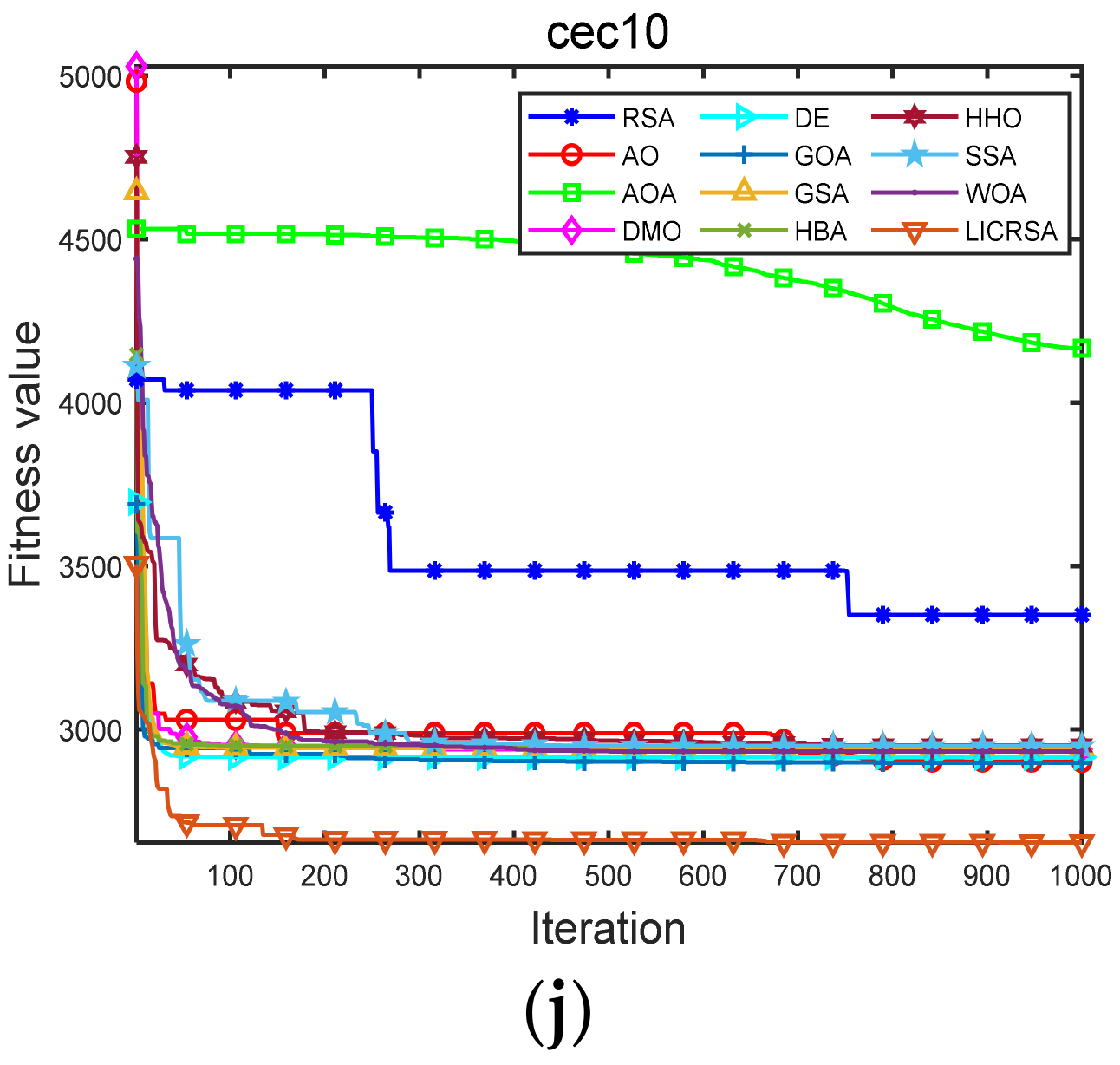
 Figure 9 and Figure 10 provide the iterative and box-line plots for the 10 test functions of this test set, respectively, from which it is found that LICRSA can find the neighborhood of the optimal case in the earlier part of the iteration for most of the test functions, and has a faster convergence rate compared to the other comparative search algorithms. Additionally, in Figure 10 it can be found that LICRSA tends to have a narrower box. It has very stable results when run many times. 
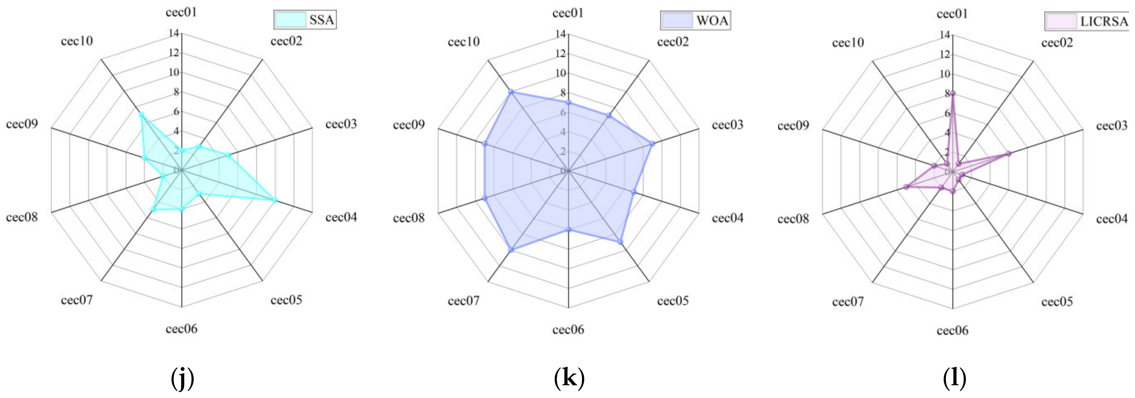
Figure 11 provides the radar plots of the 12 algorithms, and the more concentrated shaded parts represent a smaller rank ranking and better performance in CEC2020. It can be seen from the figure that LICRSA has a more minor shaded part.
Table 5 and Table 6 provide the p-values of all the search algorithms run in the CEC2020 test set and the running time statistics, respectively. From the tables, it can be found that RSA, AO, AOA, DMO, DE, and GOA are 0/1/9, 1/3/6, 0/2/8, 3/2/5, 0/3/7, 1/1/8, while GSA, HBA, HHO, SSA, and WOA are 3/1/6, 3/4/3, 1/1/8, 3/1/6, 1/0/9. In Table 6, it can be found that LICRSA takes a longer running time, but the increase in running time is a typical situation due to the added improvement policy, while the running time of RSA itself is longer, and the increase in running time of LICRSA compared to RSA is not too much.

5. Case Studies of Real-World Applications

In this section, the performance of LICRSA is further evaluated through five engineering optimization examples. Also, in this experiment, the constraints are treated by linearly weighting the constraints into the objective function. This approach is commonly used [54]. Typically, the optimization equation with a minimization objective is defined as:
Minimize:
f(Z), Z = [z1, z2, … zn]
Subject to:
g i ( Z ) 0 ,     i = 1 , , m . h j ( Z ) = 0 ,     j = 1 , , l .
where m is the number of constraints and l is the number of equilibrium constraints. Z is a candidate solution that is in the feasible domain. Thus, the equation after linear weighting of the constraints to the objective function is described as:
f ( Z ) = f ( Z ) + α i = 1 m max { g i ( Z ) ,   0 } + β j = 1 l max { h j ( Z ) ,   0 } .
where α is the weight of g(Z), and β is the weight of h(Z). In the practical case, to ensure that the solution is in the feasible domain, the candidate solution is severely penalized by larger weights on the objective function when the g(Z) and h(Z) constraints are exceeded.

5.1. Welded Beam Design Problem

The ultimate goal of the welded beam design optimization is to minimize the fabrication cost of the welded beam. Four decision variables exist for this design problem, namely: the thickness of the weld (h), length of the connected part of the reinforcement (l), the height of the reinforcement (t), and thickness of the reinforcement (b), with seven constraints [4]. The schematic diagram of the welded beam is provided in Figure 12. The mathematical expression of the welded beam optimization is as follows.
Minimize:
f ( x ) = 1.10471 x 1 2 x 2 + 0.04811 x 3 x 4 ( 14.0 + x 2 ) ,
Subject to:
g 1 ( x ) = τ ( x ) τ max 0 ,
g 2 ( x ) = σ ( x ) σ max 0 ,
g 3 ( x ) = δ ( x ) δ max 0 ,
g 4 ( x ) = x 1 x 4 0 ,
g 5 ( x ) = P P C ( x ) 0 ,
g 6 ( x ) = 0.125 x 1 0 ,
g 7 ( x ) = 1.10471 x 1 2 + 0.04811 x 3 x 4 ( 14.0 + x 2 ) 5.0 0 ,
where,
τ ( x ) = ( τ ) 2 + 2 τ τ x 2 R + ( τ ) 2 ,
τ = P 2 x 1 x 2 , τ = M R J ,
M = P ( L + x 2 2 ) ,
R = x 2 2 4 + ( x 1 + x 3 2 ) 2 ,
J = 2 2 x 1 x 2 x 2 2 4 + x 1 + x 3 2 2 ,
σ ( x ) = 6 P L x 4 x 3 2 , δ ( x ) = 6 P L 3 E x 3 2 x 4 ,
P c ( x ) = x 3 2 x 4 6 36 4.013 E L 2 1 x 3 2 L E 4 G   ,
P = 6000   l b , L = 14   i n , δ max = 0.25   i n , E = 30 × 1 6 p s i ,
G = 12 × 10 6 p s i , τ max = 13,600 p s i , σ max = 30,000 p s i
Variable range:
0.1 x 1 2 , 0.1 x 2 10 ,
Eleven authoritative and most popular algorithms (AOA [4], WCA [55], EPO [56], LSA [40], GOA [18], ASO [29], GSA [33], HHO [8], SCA [42], WHOA [15], SSA [11]) are selected to ensure reliability during the experimental demonstration and compared with the results of LICRSA for solving and optimizing the welded beam design. The numerical results are presented in Table 7, which displays the design variables and minimum expenditures for each algorithm optimization, and Table 8 provides the statistics for 20 runs. In addition, Table 9 provides the algorithms from the literature (AOA [4], WCA [55], EPO [56], AHA [57], DMO [6], SO [58], HHO [8], SSA [11], COOT [14], HBA [52]. GJO [59]) obtained. The table displays that LICRSA finds the optimal results and design variables for the welded beam design. The results show that LICRSA is one of the excellent methods to solve the problem.

5.2. Pressure Vessel Design Problem

The ultimate requirement for pressure vessel design is to minimize the cost of fabrication, welding, and materials for the pressure vessel [4]. Figure 13 prompts us that a hemispherical head capped the cylindrical vessel at both ends. Four relevant design variables need to be considered for optimization, including shell thickness Ts (x1), head thickness Th (x2), internal diameter R (x3), and vessel cylindrical cross-section length L (x4). The mathematical optimization model for pressure vessel design is as follows:
Minimize:
f ( x ) = 0.6224 x 1 x 3 x 4 + 1.7781 x 2 x 3 2 + 3.1661 x 1 2 x 4 + 19.84 x 1 2 x 3 ,
Subject to:
g 1 ( x ) = x 1 + 0.0193 x 3 0 ,
g 2 ( x ) = x 2 + 0.00954 x 3 0 ,
g 3 ( x ) = π x 3 2 x 4 4 3 π x 3 3 + 1 , 296 , 000 0 ,
g 4 ( x ) = x 4 240 0 ,
Variable range:
0 x 1 , x 2 99 ,
10 x 3 , x 4 200 ,
In this section, eleven different MH algorithms (AOA [4], CSO [48], HHO [8], BOA [26], GSA [33], GBO [13], SMA [22], SSA [11], COOT [14], HGS [39], AO [23]) are used to compare with the experimental results of LICRSA and provide the experimental results. Among them, Table 10 provides the optimization results for the four design variables and the minimum overall cost. Table 11 provides the statistics for 20 independent runs. In addition, Table 12 provides the results obtained by the algorithms (AOA [4], HHO [8], SMA [22], AO [23], SO [58], GJO [59], AVOA [60], AHA [57], COOT [14], SMO [5], CSA [61]) in the literature. According to the table, LICRSA has a minimum cost of 6014.62661, and the results also prove that LICRSA can handle the pressure vessel design problem very well.

5.3. Three-Bar Truss Design Problem

The ultimate goal of the three-bar truss design is to minimize the volume of a statically loaded three-bar truss constrained by the stresses (σ) in each bar. Two design variables exist for this problem as cross-sectional area A1 = x1 and cross-sectional area A2 = x2. A schematic design of the triple truss is given in Figure 14 [5]. The mathematical optimization model of the three-bar truss design is shown below.
Minimize:
f ( x ) = ( 2 2 x 1 + x 2 ) l ,
Subject to:
g 1 ( x ) = 2 x 1 + x 2 2 x 1 2 + 2 x 1 x 2 P σ 0 ,
g 2 ( x ) = x 2 2 x 1 2 + 2 x 1 x 2 P σ 0 ,
g 3 ( x ) = 1 2 x 2 + x 1 P σ 0 ,
Variable range:
0 x 1 , x 2 1 ,
where,
l = 100   cm , P = 2   KN / cm 2 , σ = 2   KN / cm 2 .
The experiments of LICRSA and other well-known MH techniques (ASO [29], SCA [42], CSO [48], G-QPSO [62], AO [23], GSA [33], HHO [8], GWO [20], SSA [11], JS [16], GBO [13]) are provided in Table 13. It is clear from the experimental results that LICRSA outperforms selected optimization methods. The statistical results of various optimizers, including the LICRSA, are shown in Table 14. In addition, Table 15 provides the results obtained by the algorithms (CS [63], AOA [4], GBO [13], GOA [18], MVO [64], GJO [59], SSA [11], HHO [8], AVOA [60], SMO [5], CSA [61]) in the literature. The numerical results in the table prove that LICRSA can find the best minimum volume.

5.4. Rolling Element Bearing Design

The ultimate goal of a rolling element bearing is to increase the dynamic load of the rolling bearing as much as possible. Ten design variables and nine nonlinear constraints exist for the design of rolling element bearings. These ten different design variables are ball diameter Db, pitch diameter Dm, inner and outer raceway curvature coefficients fi and f0, the number of ball Z, KDmin, KDmax, ε , e, and ζ . In addition, five of the design parameters (KDmin, KDmax, ε , e, and ζ ) exist only in the constraints and are not in the objective function, so they will indirectly radiate to the internal geometry. Let [x1, x2, x3, x4, x5, x6, x7, x8, x9, x10] = [Db, Dm, fi, f0, Z, KDmin, KDmax, ε , e, and ζ ]. A schematic diagram of the rolling element bearing structure is shown in Figure 15. The mathematical optimization of the rolling element bearing is formulated as follows.
Minimize:
f ( x ¯ ) = f c Z 2 / 3 D b 1.8 ,                         if   D b 25.4 mm 3.647 f c Z 2 / 3 D b 1.4 ,     otherwise
Subject to:
g 1 ( x ¯ ) = Z ϕ 0 2 sin 1 ( D b / D m ) 1 0 ,
g 2 ( x ¯ ) = K Dmin ( D d ) 2 D b 0 ,
g 3 ( x ¯ ) = 2 D b K Dmax ( D d ) 0 ,
g 4 ( x ¯ ) = D b ζ B w 0 ,
g 5 ( x ¯ ) = 0.5 ( D + d ) D m 0 ,
g 6 ( x ¯ ) = D m ( 0.5 + e ) ( D + d ) 0 ,
g 7 ( x ¯ ) = ε D b 0.5 ( D D m D b ) 0 ,
g 8 ( x ¯ ) = 0.515 f i 0 ,
g 9 ( x ¯ ) = 0.515 f 0 0 ,
where,
f c = 37.91 1 + 1.04 1 γ 1 + γ 1.72 f i ( 2 f 0 1 ) f 0 ( 2 f i 1 ) 0.41 10 / 3 0.3 ,
γ = D b cos ( α ) D m , f i = r i D b , f 0 = r 0 D b ,
ϕ 0 = 2 π 2 cos 1 { ( D d ) / 2 3 ( T / 4 ) } 2 + { D / 2 ( T / 4 ) D b } 2 { d / 2 + ( T / 4 ) } 2 2 { ( D d ) / 2 3 ( T / 4 ) } { D / 2 ( T / 4 ) D b } ,
T D d 2 D b , D = 160 , d = 90 , B w = 30 .
with bounds:
0.5 ( D + d ) D m 0.6 ( D + d ) ,
0.15 ( D d ) D b 0.45 ( D d ) ,
4 Z 50 , 0.515 f 0 0.6 ,
0.4 K Dmin 0.5 , 0.6 K Dmax 0.7 ,
0.3 ε 0.4 , 0.02 e 0.1 , 0.6 ζ 0.85 .
Table 16 provides the design variables and optimal dynamic loads for LICRSA and eleven other MH algorithms (G-QPSO [62], AOA [4], SOA [51], WOA [24], SSA [11], SCA [42], AO [23], CSO [48], HGS [39], HHO [8], HBA [52]). Table 17 provides the statistics for 20 independent runs. In addition, Table 18 provides the results obtained by the algorithms (AHA [57], AVOA [60], HBO [65], GBO [13], CSA [61], TSA [66], SOA [51], EPO [56], MVO [64], COOT [14], HHO [8]) in the literature. The LICRSA can find the optimal design variables and dynamic loading. Thus, LICRSA proves to be a great advantage in dealing with the problem.

5.5. Speed Reducer Design

Reducers are one of the most critical components of a gearbox system. The ultimate requirement for the gearbox is weight minimization while satisfying 11 constraints. In addition, seven design variables exist for this design. x1 is the face width, x2 is the tooth mode, x3 represents the number of teeth in the pinion, x4 represents the length of the first shaft between the bearings, the length of the second shaft between the bearings is x5, and x6 and x7 represent the diameters of the first shaft and the second shaft. Figure 16 provides a schematic diagram of the reducer [5]. Also, the mathematical design equation for the reducer design is as follows.
Minimize:
f ( x ) = 0.7854 x 1 x 2 2 ( 3.3333 x 3 2 + 14.9334 x 3 43.0934 ) 1.508 x 1 ( x 6 2 + x 7 2 ) + 7.4777 ( x 6 3 + x 7 3 ) ,
Subject to:
g 1 ( x ) = 27 x 1 x 2 2 x 3 1 0 ,
g 2 ( x ) = 397.5 x 1 x 2 2 x 3 2 1 0 ,
g 3 ( x ) = 1.93 x 4 3 x 2 x 3 x 6 4 1 0 ,
g 4 ( x ) = 1.93 x 5 3 x 2 x 3 x 7 4 1 0 ,
g 5 ( x ) = ( 745 x 4 x 2 x 3 ) 2 + 16.9 × 10 6 110.0 x 6 3 1 0 ,
g 6 ( x ) = ( 745 x 4 x 2 x 3 ) 2 + 157.5 × 10 6 85.0 x 6 3 1 0 ,
g 7 ( x ) = x 2 x 3 40 1 0 ,
g 8 ( x ) = 5 x 2 x 1 1 0 ,
g 9 ( x ) = x 1 12 x 2 1 0 ,
g 10 ( x ) = 1.5 x 6 + 1.9 x 4 1 0 ,
g 11 ( x ) = 1.1 x 7 + 1.9 x 5 1 0 ,
Variable range:
2.6 x 1 3.6 , 0.7 x 2 0.8 ,
17 x 3 28 , 7.3 x 4 8.3 ,
7.8 x 5 8.3 , 2.9 x 6 3.9 , 5 x 7 5.5 .
Table 19 provides the optimal design variables and minimum weights for LICRSA and 11 other MH algorithms (LSO [67], BAT [9], BOA [26], DMO [6], SCA [41], WOA [24], HHO [8], SSA [11], CSO [48], GWO [20], SCSO [41]) for the reducer problem. Table 20 provides the statistics for 20 independent runs. In addition, Table 21 provides the results obtained by the algorithms (GOA [18], GSA [33], SCA [42], EA [68], FA [69], AO [23], MVO [64], GWO [20], CS [63], MFO [19], AOA [4]) in the literature. The results show that LICRSA achieves the best result among the search algorithms for both minimum weights. Therefore, LICRSA can solve the reducer problem well.

6. Discussion

According to the numerical situation of this study, the proposed LICRSA algorithm shows excellent performance compared with other optimization algorithms. The validation experiments are divided into three main parts. The first part compares the LICRSA algorithm with the original RSA and different optimization algorithms on 23 test functions. The LICRSA algorithm ranks first in 10 functions, accounting for 43% of all functions. In addition, the LICRSA algorithm outperforms RSA in 15 functions, implying that introducing the Lévy flight and interactive crossover strategy enhances the exploration and development capabilities. The second part compares the LICRSA algorithm with other optimization algorithms in the CEC2020 test set. After analyzing the comparative metrics such as best, mean, worst, and std of solving the benchmark function, the LICRSA also solves the test function with higher accuracy, better stability, and faster convergence. The final section will discuss the capability of LICRSA with different algorithms in solving five complex engineering examples. The simulation results verify the usefulness and dependability of the LICRSA algorithm for real optimization problems. Of course, there is room for improved algorithm stability when solving engineering optimization problems.

7. Conclusions

This paper proposes an improved reptile search algorithm based on Lévy flight and interactive crossover strategies. To improve the performance of the original RSA algorithm, two main approaches are employed to address its shortcomings. As a general modification technique to improve its optimization capability, the Lévy flight strategy enhances the global exploration of the algorithm and jumps out of local solutions. Meanwhile, the interactive crossover strategy, as a variant of the crossover operator, inherits the local exploitation ability and enhances the fit with iterations. Twenty-three benchmark test functions, the IEEE Conference Evolutionary Computation (CEC2020) benchmark, and five engineering design problems are used to test the proposed LICRSA algorithm and verify the effectiveness of LICRSA. The experimental results show that LICRSA obtains more suitable optimization results and significantly outperforms competing algorithms, including DMO, WOA, HHO, DE, AOA, and WSO. The LICRSA has a more significant global search capability and higher accuracy solutions. In addition, the results of the tested mechanical engineering problems prove that LICRSA outperforms other optimization methods in total cost evaluation criteria. LICRSA has excellent performance and can be utilized by other researchers to tackle complex optimization problems.
Similarly, the applicability of RSA will be investigated. For example, to further improve the spatial search capability, we try to integrate RSA with other general intelligent group algorithms to improve the global performance of RSA. We use RSA to provide optimal parameters for machine learning models in privacy-preserving and social networks in practical applications. Furthermore, the proposed LICRSA algorithm may also have excellent application potency in solving other complex optimization problems, such as shop scheduling problems [70], optimal degree reduction [71], image segmentation [72], shape optimization [73], and feature selection [74], etc.

Author Contributions

Conceptualization, L.H. and G.H.; Data curation, Y.W. and Y.G.; Formal analysis, L.H., Y.W. and Y.G.; Funding acquisition, L.H. and G.H.; Investigation, L.H., Y.W., Y.G. and G.H.; Methodology, L.H., Y.W., Y.G. and G.H.; Resources, L.H. and G.H.; Software, L.H., Y.W. and Y.G.; Supervision, G.H.; Validation, G.H.; Visualization, Y.W. and Y.G.; Writing—original draft, L.H., Y.W., Y.G. and G.H.; Writing—review & editing, L.H. and G.H. All authors have read and agreed to the published version of the manuscript.

Funding

This work is supported by the Research Fund of Department of Science and Department of Education of Shaanxi, China (Grant No. 21JK0615).

Institutional Review Board Statement

Not applicable.

Informed Consent Statement

Not applicable.

Data Availability Statement

All data generated or analyzed during this study were included in this published article.

Conflicts of Interest

The authors declare no conflict of interest.

References

  1. Houssein, E.H.; Rezk, H.; Fathy, A.; Mahdy, M.A.; Nassef, A.M. A modified adaptive guided differential evolution algorithm applied to engineering applications. Eng. Appl. Artif. Intell. 2022, 113, 104920. [Google Scholar] [CrossRef]
  2. Minh, H.-L.; Sang-To, T.; Wahab, M.A.; Cuong-Le, T. A new metaheuristic optimization based on K-means clustering algorithm and its application for structural damage identification in a complex 3D concrete structure. Knowl.-Based Syst. 2022, 251, 109189. [Google Scholar] [CrossRef]
  3. Hu, G.; Zhong, J.; Du, B.; Wei, G. An enhanced hybrid arithmetic optimization algorithm for engineering applications. Comput. Methods Appl. Mech. Eng. 2022, 394, 114901. [Google Scholar] [CrossRef]
  4. Abualigah, L.; Diabat, A.; Mirjalili, S.; Abd Elaziz, M.; Gandomi, A.H. The Arithmetic Optimization Algorithm. Comput. Methods Appl. Mech. Eng. 2021, 376, 113609. [Google Scholar] [CrossRef]
  5. Zamani, H.; Nadimi-Shahraki, M.H.; Gandomi, A.H. Starling murmuration optimizer: A novel bio-inspired algorithm for global and engineering optimization. Comput. Methods Appl. Mech. Eng. 2022, 392, 114616. [Google Scholar] [CrossRef]
  6. Agushaka, J.O.; Ezugwu, A.E.; Abualigah, L. Dwarf Mongoose Optimization Algorithm. Comput. Methods Appl. Mech. Eng. 2022, 391, 114570. [Google Scholar] [CrossRef]
  7. Abualigah, L.; Elaziz, M.A.; Sumari, P.; Geem, Z.W.; Gandomi, A.H. Reptile Search Algorithm (RSA): A nature-inspired meta-heuristic optimizer. Expert Syst. Appl. 2022, 191, 116158. [Google Scholar] [CrossRef]
  8. Heidari, A.A.; Mirjalili, S.; Faris, H.; Aljarah, I.; Mafarja, M.; Chen, H. Harris hawks optimization: Algorithm and applications. Future Gener. Comput. Syst. 2019, 97, 849–872. [Google Scholar] [CrossRef]
  9. Gupta, D.; Arora, J.; Agrawal, U.; Khanna, A.; de Albuquerque, V.H.C. Optimized Binary Bat algorithm for classification of white blood cells. Measurement 2019, 143, 180–190. [Google Scholar] [CrossRef]
  10. Premkumar, M.; Jangir, P.; Sowmya, R. MOGBO: A new Multiobjective Gradient-Based Optimizer for real-world structural optimization problems. Knowl.-Based Syst. 2021, 218, 106856. [Google Scholar] [CrossRef]
  11. Mirjalili, S.; Gandomi, A.H.; Mirjalili, S.Z.; Saremi, S.; Faris, H.; Mirjalili, S.M. Salp Swarm Algorithm: A bio-inspired optimizer for engineering design problems. Adv. Eng. Softw. 2017, 114, 163–191. [Google Scholar] [CrossRef]
  12. Hu, G.; Zhu, X.; Wei, G.; Chang, C.-T. An improved marine predators algorithm for shape optimization of developable Ball surfaces. Eng. Appl. Artif. Intell. 2021, 105, 104417. [Google Scholar] [CrossRef]
  13. Ahmadianfar, I.; Bozorg-Haddad, O.; Chu, X. Gradient-based optimizer: A new metaheuristic optimization algorithm. Inf. Sci. 2020, 540, 131–159. [Google Scholar] [CrossRef]
  14. Naruei, I.; Keynia, F. A new optimization method based on COOT bird natural life model. Expert Syst. Appl. 2021, 183, 115352. [Google Scholar] [CrossRef]
  15. Naruei, I.; Keynia, F. Wild horse optimizer: A new meta-heuristic algorithm for solving engineering optimization problems. Eng. Comput. 2021. [Google Scholar] [CrossRef]
  16. Chou, J.-S.; Truong, D.-N. A novel metaheuristic optimizer inspired by behavior of jellyfish in ocean. Appl. Math. Comput. 2021, 389, 125535. [Google Scholar] [CrossRef]
  17. Gandomi, A.H.; Alavi, A.H. Krill herd: A new bio-inspired optimization algorithm. Commun. Nonlinear Sci. Numer. Simul. 2012, 17, 4831–4845. [Google Scholar] [CrossRef]
  18. Saremi, S.; Mirjalili, S.; Lewis, A. Grasshopper Optimisation Algorithm: Theory and application. Adv. Eng. Softw. 2017, 105, 30–47. [Google Scholar] [CrossRef] [Green Version]
  19. Mirjalili, S. Moth-flame optimization algorithm: A novel nature-inspired heuristic paradigm. Knowl.-Based Syst. 2015, 89, 228–249. [Google Scholar] [CrossRef]
  20. Mirjalili, S.; Mirjalili, S.M.; Lewis, A. Grey Wolf Optimizer. Adv. Eng. Softw. 2014, 69, 46–61. [Google Scholar] [CrossRef] [Green Version]
  21. Połap, D.; Woźniak, M. Red fox optimization algorithm. Expert Syst. Appl. 2021, 166, 114107. [Google Scholar] [CrossRef]
  22. Li, S.; Chen, H.; Wang, M.; Heidari, A.A.; Mirjalili, S. Slime mould algorithm: A new method for stochastic optimization. Future Gener. Comput. Syst. 2020, 111, 300–323. [Google Scholar] [CrossRef]
  23. Abualigah, L.; Yousri, D.; Abd Elaziz, M.; Ewees, A.A.; Al-qaness, M.A.A.; Gandomi, A.H. Aquila Optimizer: A novel meta-heuristic optimization algorithm. Comput. Ind. Eng. 2021, 157, 107250. [Google Scholar] [CrossRef]
  24. Mirjalili, S.; Lewis, A. The Whale Optimization Algorithm. Adv. Eng. Softw. 2016, 95, 51–67. [Google Scholar] [CrossRef]
  25. Xue, J.; Shen, B. A novel swarm intelligence optimization approach: Sparrow search algorithm. Syst. Sci. Control. Eng. 2020, 8, 22–34. [Google Scholar] [CrossRef]
  26. Arora, S.; Singh, S. Butterfly optimization algorithm: A novel approach for global optimization. Soft Comput. 2019, 23, 715–734. [Google Scholar] [CrossRef]
  27. Beyer, H.-G.; Schwefel, H.-P. Evolution strategies—A comprehensive introduction. Nat. Comput. 2002, 1, 3–52. [Google Scholar] [CrossRef]
  28. Pourpasha, H.; Farshad, P.; Zeinali Heris, S. Modeling and optimization the effective parameters of nanofluid heat transfer performance using artificial neural network and genetic algorithm method. Energy Rep. 2021, 7, 8447–8464. [Google Scholar] [CrossRef]
  29. Zhao, W.; Wang, L.; Zhang, Z. Atom search optimization and its application to solve a hydrogeologic parameter estimation problem. Knowl.-Based Syst. 2019, 163, 283–304. [Google Scholar] [CrossRef]
  30. Kaveh, A.; Dadras, A. A novel meta-heuristic optimization algorithm: Thermal exchange optimization. Adv. Eng. Softw. 2017, 110, 69–84. [Google Scholar] [CrossRef]
  31. Al-Madi, N.; Faris, H.; Mirjalili, S. Binary multi-verse optimization algorithm for global optimization and discrete problems. Int. J. Mach. Learn. Cybern. 2019, 10, 3445–3465. [Google Scholar] [CrossRef]
  32. Lam, A.Y.S.; Li, V.O.K. Chemical Reaction Optimization: A tutorial. Memet. Comput. 2012, 4, 3–17. [Google Scholar] [CrossRef] [Green Version]
  33. Rashedi, E.; Nezamabadi-pour, H.; Saryazdi, S. GSA: A Gravitational Search Algorithm. Inf. Sci. 2009, 179, 2232–2248. [Google Scholar] [CrossRef]
  34. Mousavirad, S.J.; Ebrahimpour-Komleh, H. Human mental search: A new population-based metaheuristic optimization algorithm. Appl. Intell. 2017, 47, 850–887. [Google Scholar] [CrossRef]
  35. Das, B.; Mukherjee, V.; Das, D. Student psychology based optimization algorithm: A new population based optimization algorithm for solving optimization problems. Adv. Eng. Softw. 2020, 146, 102804. [Google Scholar] [CrossRef]
  36. Rao, R.V.; Savsani, V.J.; Vakharia, D.P. Teaching—Learning-based optimization: A novel method for constrained mechanical design optimization problems. Comput. Aided Des. 2011, 43, 303–315. [Google Scholar] [CrossRef]
  37. Hu, G.; Du, B.; Wang, X.; Wei, G. An enhanced black widow optimization algorithm for feature selection. Knowl.-Based Syst. 2022, 235, 107638. [Google Scholar] [CrossRef]
  38. Hu, G.; Li, M.; Wang, X.; Wei, G.; Chang, C.-T. An enhanced manta ray foraging optimization algorithm for shape optimization of complex CCG-Ball curves. Knowl.-Based Syst. 2022, 240, 108071. [Google Scholar] [CrossRef]
  39. Yang, Y.; Chen, H.; Heidari, A.A.; Gandomi, A.H. Hunger games search: Visions, conception, implementation, deep analysis, perspectives, and towards performance shifts. Expert Syst. Appl. 2021, 177, 114864. [Google Scholar] [CrossRef]
  40. Shareef, H.; Ibrahim, A.A.; Mutlag, A.H. Lightning search algorithm. Appl. Soft Comput. 2015, 36, 315–333. [Google Scholar] [CrossRef]
  41. Seyyedabbasi, A.; Kiani, F. Sand Cat swarm optimization: A nature-inspired algorithm to solve global optimization problems. Eng. Comput. 2022. [Google Scholar] [CrossRef]
  42. Mirjalili, S. SCA: A Sine Cosine Algorithm for solving optimization problems. Knowl.-Based Syst. 2016, 96, 120–133. [Google Scholar] [CrossRef]
  43. Zhou, B.; Lei, Y. Bi-objective grey wolf optimization algorithm combined Levy flight mechanism for the FMC green scheduling problem. Appl. Soft Comput. 2021, 111, 107717. [Google Scholar] [CrossRef]
  44. Zhang, Y.; Jin, Z.; Zhao, X.; Yang, Q. Backtracking search algorithm with Lévy flight for estimating parameters of photovoltaic models. Energy Convers. Manag. 2020, 208, 112615. [Google Scholar] [CrossRef]
  45. Dinkar, S.K.; Deep, K. An efficient opposition based Lévy Flight Antlion optimizer for optimization problems. J. Comput. Sci. 2018, 29, 119–141. [Google Scholar] [CrossRef]
  46. Feng, Z.-K.; Liu, S.; Niu, W.-J.; Li, S.-S.; Wu, H.-J.; Wang, J.-Y. Ecological operation of cascade hydropower reservoirs by elite-guide gravitational search algorithm with Lévy flight local search and mutation. J. Hydrol. 2020, 581, 124425. [Google Scholar] [CrossRef]
  47. Gao, J.; Gao, F.; Ma, Z.; Huang, N.; Yang, Y. Multi-objective optimization of smart community integrated energy considering the utility of decision makers based on the Lévy flight improved chicken swarm algorithm. Sustain. Cities Soc. 2021, 72, 103075. [Google Scholar] [CrossRef]
  48. Meng, A.-B.; Chen, Y.-C.; Yin, H.; Chen, S.-Z. Crisscross optimization algorithm and its application. Knowl.-Based Syst. 2014, 67, 218–229. [Google Scholar] [CrossRef]
  49. Storn, R.; Price, K. Differential Evolution—A Simple and Efficient Heuristic for Global Optimization over Continuous Spaces. J. Glob.Optim. 1997, 11, 341–359. [Google Scholar] [CrossRef]
  50. Braik, M.; Hammouri, A.; Atwan, J.; Al-Betar, M.A.; Awadallah, M.A. White Shark Optimizer: A novel bio-inspired meta-heuristic algorithm for global optimization problems. Knowl.-Based Syst. 2022, 243, 108457. [Google Scholar] [CrossRef]
  51. Dhiman, G.; Kumar, V. Seagull optimization algorithm: Theory and its applications for large-scale industrial engineering problems. Knowl.-Based Syst. 2019, 165, 169–196. [Google Scholar] [CrossRef]
  52. Hashim, F.A.; Houssein, E.H.; Hussain, K.; Mabrouk, M.S.; Al-Atabany, W. Honey Badger Algorithm: New metaheuristic algorithm for solving optimization problems. Math. Comput. Simul. 2022, 192, 84–110. [Google Scholar] [CrossRef]
  53. Hussain, K.; Salleh, M.N.M.; Cheng, S.; Shi, Y. On the exploration and exploitation in popular swarm-based metaheuristic algorithms. Neural Comput. Appl. 2019, 31, 7665–7683. [Google Scholar] [CrossRef]
  54. Coello Coello, C.A. Theoretical and numerical constraint-handling techniques used with evolutionary algorithms: A survey of the state of the art. Methods Appl. Mech. Eng. 2002, 191, 1245–1287. [Google Scholar] [CrossRef]
  55. Eskandar, H.; Sadollah, A.; Bahreininejad, A.; Hamdi, M. Water cycle algorithm—A novel metaheuristic optimization method for solving constrained engineering optimization problems. Comput. Struct. 2012, 110–111, 151–166. [Google Scholar] [CrossRef]
  56. Dhiman, G.; Kumar, V. Emperor penguin optimizer: A bio-inspired algorithm for engineering problems. Knowl.-Based Syst. 2018, 159, 20–50. [Google Scholar] [CrossRef]
  57. Zhao, W.; Wang, L.; Mirjalili, S. Artificial hummingbird algorithm: A new bio-inspired optimizer with its engineering applications. Comput. Methods Appl. Mech. Eng. 2022, 388, 114194. [Google Scholar] [CrossRef]
  58. Hashim, F.A.; Hussien, A.G. Snake Optimizer: A novel meta-heuristic optimization algorithm. Knowl.-BasedSyst. 2022, 242, 108320. [Google Scholar] [CrossRef]
  59. Chopra, N.; Mohsin Ansari, M. Golden jackal optimization: A novel nature-inspired optimizer for engineering applications. Expert Syst. Appl. 2022, 198, 116924. [Google Scholar] [CrossRef]
  60. Abdollahzadeh, B.; Gharehchopogh, F.S.; Mirjalili, S. African vultures optimization algorithm: A new nature-inspired metaheuristic algorithm for global optimization problems. Comput. Ind. Eng. 2021, 158, 107408. [Google Scholar] [CrossRef]
  61. Braik, M.S. Chameleon Swarm Algorithm: A bio-inspired optimizer for solving engineering design problems. Expert Syst. Appl. 2021, 174, 114685. [Google Scholar] [CrossRef]
  62. Dos Santos Coelho, L. Gaussian quantum-behaved particle swarm optimization approaches for constrained engineering design problems. Expert Syst. Appl. 2010, 37, 1676–1683. [Google Scholar] [CrossRef]
  63. Gandomi, A.H.; Yang, X.-S.; Alavi, A.H. Cuckoo search algorithm: A metaheuristic approach to solve structural optimization problems. Eng. Comput. 2013, 29, 17–35. [Google Scholar] [CrossRef]
  64. Mirjalili, S.; Mirjalili, S.M.; Hatamlou, A. Multi-Verse Optimizer: A nature-inspired algorithm for global optimization. Neural Comput. Appl. 2016, 27, 495–513. [Google Scholar] [CrossRef]
  65. Askari, Q.; Saeed, M.; Younas, I. Heap-based optimizer inspired by corporate rank hierarchy for global optimization. Expert Syst. Appl. 2020, 161, 113702. [Google Scholar] [CrossRef]
  66. Kaur, S.; Awasthi, L.K.; Sangal, A.L.; Dhiman, G. Tunicate Swarm Algorithm: A new bio-inspired based metaheuristic paradigm for global optimization. Eng. Appl. Artif. Intell. 2020, 90, 103541. [Google Scholar] [CrossRef]
  67. Liu, J.; Li, D.; Wu, Y.; Liu, D. Lion swarm optimization algorithm for comparative study with application to optimal dispatch of cascade hydropower stations. Appl. Soft Comput. 2020, 87, 105974. [Google Scholar] [CrossRef]
  68. Mezura-Montes, E.; Coello, C.A.C.; Landa-Becerra, R. Engineering optimization using simple evolutionary algorithm. In Proceedings of the 15th IEEE International Conference on Tools with Artificial Intelligence, Sacramento, CA, USA, 5 November 2003; pp. 149–156. [Google Scholar]
  69. Baykasoğlu, A.; Ozsoydan, F.B. Adaptive firefly algorithm with chaos for mechanical design optimization problems. Appl. Soft Comput. 2015, 36, 152–164. [Google Scholar] [CrossRef]
  70. Ghasemi, A.; Ashoori, A.; Heavey, C. Evolutionary Learning Based Simulation Optimization for Stochastic Job Shop Scheduling Problems. Appl. Soft Comput. 2021, 106, 107309. [Google Scholar] [CrossRef]
  71. Hu, G.; Dou, W.; Wang, X.; Abbas, M. An enhanced chimp optimization algorithm for optimal degree reduction of Said–Ball curves. Math. Comput. Simul. 2022, 197, 207–252. [Google Scholar] [CrossRef]
  72. Larabi Marie-Sainte, S.; Alskireen, R.; Alhalawani, S. Emerging Applications of Bio-Inspired Algorithms in Image Segmentation. Electronics 2021, 10, 3116. [Google Scholar] [CrossRef]
  73. Zheng, J.; Hu, G.; Ji, X.; Qin, X. Quintic generalized Hermite interpolation curves: Construction and shape optimization using an improved GWO algorithm. Comput. Appl. Math. 2022, 41, 115. [Google Scholar] [CrossRef]
  74. Wang, X.; Wang, Y.; Wong, K.-C.; Li, X. A self-adaptive weighted differential evolution approach for large-scale feature selection. Knowl.-Based Syst. 2022, 235, 107633. [Google Scholar] [CrossRef]
Figure 1. The introduction diagram of the interaction crossover.
Mathematics 10 02329 g001
Figure 2. Flowchart for the LICRSA algorithm.
Mathematics 10 02329 g002
Figure 3. The exploration and exploitation behavior: (a) cec02; (b) cec04; (c) cec06; (d) cec07; (e) cec08; (f) cec09.
Mathematics 10 02329 g003
Figure 4. The percentage of different functions.
Mathematics 10 02329 g004
Figure 5. Mean rank of different algorithms.
Mathematics 10 02329 g005
Figure 6. The number of better than, worse than, same as LICRSA.
Mathematics 10 02329 g006
Figure 7. Convergence curves of LICRSA and different MH algorithms: (a) F01; (b) F02; (c) F03; (d) F04; (e) F05; (f) F06; (g) F07; (h) F08; (i) F09; (j) F10; (k) F11; (l) F12; (m) F13; (n) F14; (o) F15; (p) F16; (q) F17; (r) F18; (s) F19; (t) F20; (u) F21; (v) F22; (w) F23.
Mathematics 10 02329 g007aMathematics 10 02329 g007bMathematics 10 02329 g007c
Figure 8. Box plot of LICRSA and RSA, AO, AOA, CSO, DMO, DE, WSO, SOA, GSA, WHOA, WOA: (a) F01; (b) F02; (c) F03; (d) F04; (e) F05; (f) F06; (g) F07; (h) F08; (i) F09; (j) F10; (k) F11; (l) F12; (m) F13; (n) F14; (o) F15; (p) F16; (q) F17; (r) F18; (s) F19; (t) F20; (u) F21; (v) F22; (w) F23.
Mathematics 10 02329 g008aMathematics 10 02329 g008bMathematics 10 02329 g008c
Figure 9. The convergence curves of the LICRSA and search algorithms on CEC2020: (a) cec01; (b) cec02; (c) cec03; (d) cec04; (e) cec05; (f) cec06; (g) cec07; (h) cec08; (i) cec09; (j) cec10.
Mathematics 10 02329 g009aMathematics 10 02329 g009b
Figure 10. Box plot of the LICRSA and other MH algorithms on CEC2020: (a) cec01; (b) cec02; (c) cec03; (d) cec04; (e) cec05; (f) cec06; (g) cec07; (h) cec08; (i) cec09; (j) cec10.
Mathematics 10 02329 g010aMathematics 10 02329 g010b
Figure 11. Radar plot of 12 algorithms in CEC2020: (a) RSA; (b) AO; (c) AOA; (d) DMO; (e) DE; (f) GOA; (g) GSA; (h) HBA; (i) HHO; (j) SSA; (k) WOA; (l) LICRSA.
Mathematics 10 02329 g011aMathematics 10 02329 g011b
Figure 12. Welded beam design.
Mathematics 10 02329 g012
Figure 13. Pressure vessel design.
Mathematics 10 02329 g013
Figure 14. Three-bar truss design.
Mathematics 10 02329 g014
Figure 15. Rolling element bearing design.
Mathematics 10 02329 g015
Figure 16. Speed reducer design.
Mathematics 10 02329 g016
Table 1. Parameters setting.
AlgorithmParametersValues
AOA [4]µ0.499
aa5
WSO [50]fmin, fmax0.07, 0.75
τ, ao, a1, a24.125, 6.25, 100, 0.0005
GSA [33]ElitistCheck, Rpower, Rnorm, alpha, G01, 1, 2, 20, 100
WOA [24]A Decreased from 2 to 0
b2
SSA [11]Leader position update probabilityc3 = 0.5
RSA [7]α0.1
β0.1
DE [49]Scaling factor0.5
Crossover probability0.5
WHO [15]Crossover percentagePC = 0.13
Stallions percentage (number of groups)PS = 0.2
CrossoverMean
HBA [52]β (the ability of a honey badger to get food)6
C2
SOA [51]Control Parameter (A)[2, 0]
fc2
Table 2. Numerical results for best, worst, mean, std of the search algorithm in 12 of the 23 benchmark functions.
FunctionIndexAlgorithms
RSAAOAOACSODEDMOWSOWOAWHOASOAGSALICRSA
F1Best02.65 × 10−3005.12 × 10−79.24 × 10−265.35 × 10−31.07 × 10−42.5012 3.21 × 10−1666.71 × 10−10504.60 × 10−170
Worst03.34 × 10−2062.17 × 10−061.40 × 10−172.16 × 1041.44 × 10−0337.3501 9.22 × 10−1468.44 × 10−9202.55 × 10−160
Mean01.11 × 10−2071.27 × 10−66.66 × 10−192.83 × 1034.89 × 10−412.9127 3.07 × 10−1475.18 × 10−9301.27 × 10−160
Std004.26 × 10−72.63 × 10−185.08 × 1033.35 × 10−49.1243 1.68 × 10−1461.87 × 10−9205.20 × 10−170
Rank149712101156181
F2Best01.52 × 10−1531.34 × 10−92.68 × 10−167.29 × 10−33.88 × 10−40.2289 4.65 × 10−1163.79 × 10−5803.17 × 10−80
Worst01.71 × 10−992.57 × 10−33.98 × 10−1342.4839 3.7448 1.1593 1.86 × 10−1003.53 × 10−502.65 × 10−3009.93 × 10−80
Mean06.53 × 10−1013.55 × 10−41.72 × 10−147.9621 0.1367 0.5527 6.23 × 10−1021.23 × 10−512.65 × 10−3005.74 × 10−80
Std03.14 × 10−1006.00 × 10−47.21 × 10−149.8024 0.6817 0.2489 3.40 × 10−1016.44 × 10−5101.58 × 10−80
Rank159712101146381
F3Best01.17 × 10−2953.75 × 10−6141.0483 2.54 × 1032.49 × 104164.7909 6.50 × 1036.15 × 10−722.61 × 103273.2429 0
Worst02.22 × 10−1901.52 × 10−33.99 × 1037.57 × 1046.99 × 1041.09 × 1034.75 × 1042.79 × 10−553.74 × 104930.4876 0
Mean01.04 × 10−1913.16 × 10−4900.3036 2.08 × 1045.19 × 104575.8136 2.30 × 1042.24 × 10−561.31 × 104491.8570 0
Std003.36 × 10−4777.9065 1.67 × 1041.17 × 104252.9466 1.03 × 1046.90 × 10−568.92 × 103150.6003 0
Rank135810127114961
F4Best06.29 × 10−1540.0002 0.0075 45.5951 36.1441 5.3086 1.4451 4.89 × 10−413.77 × 10−1281.52 × 10−80
Worst08.32 × 10−1090.0402 0.0809 78.0134 62.1824 14.6068 87.4681 2.90 × 10−352.23 × 10−424.7297 0
Mean02.77 × 10−1100.0084 0.0330 63.6120 45.8755 10.6183 43.7648 1.49 × 10−368.93 × 10−441.4748 0
Std01.52 × 10−1090.0091 0.0205 8.1802 5.3785 2.1397 26.3941 5.37 × 10−364.10 × 10−431.5097 0
Rank136712119105481
F5Best6.72 × 10−296.83 × 10−626.6485 0.0055 869.9148 577.6902 293.4370 0.8391 24.4814 28.7246 26.0094 1.13 × 10⁻¹⁹
Worst28.9901 0.0088 28.0367 264.5424 6.96 × 1077.73 × 1032.18 × 10328.7495 78.4426 28.8734 347.4929 10.8886
Mean7.7128 0.0018 27.4318 52.0036 8.42 × 1062.67 × 103812.9171 26.3925 29.1866 28.8012 49.0518 0.4101
Std13.0090 0.0024 0.3141 61.6943 1.60 × 1072.12 × 103470.7655 4.8696 13.3897 0.0403 65.9500 1.9898
Rank315912111047682
F6Best3.5635 1.69 × 10−81.2454 5.23 × 10−250.0228 8.03 × 10−55.5298 0.0073 5.27 × 10−120.5051 3.69 × 10−170.7079
Worst7.4998 3.30 × 10−42.0581 4.44 × 10−216.98 × 1039.35 × 10−4268.0956 0.3385 1.94 × 10−64.6282 2.80 × 10−164.7392
Mean6.4884 4.93 × 10−51.7396 5.00 × 10−22710.2299 4.19 × 10−427.5978 0.0740 1.28 × 10−72.4897 1.06 × 10−161.4065
Std1.0043 7.83 × 10−50.1716 1.03 × 10−211.59 × 1032.52 × 10−447.2090 0.0920 3.67 × 10−71.0757 5.66 × 10−170.9717
Rank104811251163927
F7Best4.67 × 10−67.17 × 10−87.42 × 10−70.0003 1.9479 0.0532 0.0275 2.91 × 10−51.78 × 10−51.38 × 10−60.0275 1.56 × 10⁻⁶
Worst2.92 × 10−41.78 × 10−49.71 × 10−50.0073 45.3077 0.1374 0.3394 0.0113 0.0015 1.99 × 10−40.1400 1.47 × 10⁻⁴
Mean4.39 × 10−55.82 × 10−52.64 × 10−50.0017 8.9688 0.0849 0.1140 0.0017 0.0005 6.14 × 10−50.0623 3.62 × 10⁻⁵
Std5.97 × 10−55.03 × 10−52.12 × 10−50.0014 9.0334 0.0240 0.0822 0.0026 0.0004 5.22 × 10−50.0247 3.62 × 10⁻⁵
Rank341812101176592
F8Best−5746.50 −12,569.29 −6195.38 −12,569.49 −8839.00 −4960.68 −8910.96 −12,569.48 −10,488.23 −12,569.49 −3688.28 −6842.38
Worst−4375.91 −4200.08 −4766.89 −12,451.05 −5365.73 −3794.91 −3456.50 −7192.25 −7284.72 −12,569.47 −1665.49 −4351.51
Mean−5443.79 −9725.52 −5544.32 −12,565.05 −7455.45 −4300.56 −7038.96 −11,053.13 −9089.71 −12,569.49 −2599.01 −5782.82
Std277.88 3560.82 365.06 21.61 827.49 322.21 1276.74 1870.29 602.23 0.00 453.89 598.89
Rank104926117351128
F9Best000075.8378 146.1968 10.4790 00012.9345 0
Worst006.47 × 10−76.25 × 10−13261.5807 231.3507 33.3913 00053.7277 0
Mean001.69 × 10−79.28 × 10−14161.8547 203.2452 20.3445 00024.9735 0
Std002.08 × 10−71.17 × 10−1348.2843 19.8946 5.2764 0009.4583 0
Rank118711129111101
F10Best8.88 × 10−168.88 × 10−162.23 × 10−61.68 × 10−1319.9571 0.0039 2.3685 8.88 × 10−168.88 × 10−168.88 × 10−164.84 × 10−98.88 × 10−16
Worst8.88 × 10−168.88 × 10−163.87 × 10−49.81 × 10−1019.9753 0.0602 5.4315 7.99 × 10−157.99 × 10−158.88 × 10−161.05 × 10−88.88 × 10−16
Mean8.88 × 10−168.88 × 10−161.79 × 10−44.82 × 10−1119.9648 0.0160 3.6012 4.20 × 10−152.90 × 10−158.88 × 10−167.90 × 10−98.88 × 10−16
Std001.11 × 10−41.84 × 10−100.0035 0.0109 0.6814 2.27 × 10−152.41 × 10−1501.47 × 10−90
Rank119712101165181
F11Best003.50 × 10−600.0973 0.0017 1.0480 0002.9419 0
Worst000.0074 0.7293 53.0911 0.3955 2.0351 00013.8166 0
Mean000.0003 0.1491 9.1646 0.0460 1.1800 0007.4863 0
Std000.0013 0.2365 12.3615 0.0845 0.1848 0002.6727 0
Rank117912810111111
F12Best0.6944 1.33 × 10−80.5443 4.48 × 10−275.61 × 1035.0890 0.2155 0.0008 1.61 × 10−130.0035 3.44 × 10−190.0201
Worst1.6297 8.11 × 10−60.6527 6.41 × 10−224.86 × 10826.7847 8.2292 0.1443 0.1037 0.7420 1.4406 1.1004
Mean1.2466 1.16 × 10−60.5999 3.78 × 10−232.95 × 10713.8952 1.5707 0.0112 0.0138 0.1820 0.1335 0.2364
Std0.3311 1.66 × 10−60.0291 1.35 × 10−229.56 × 1075.2129 1.5644 0.0262 0.0358 0.1907 0.2965 0.2769
Rank928112111034657
F13Best6.28 × 10−321.50 × 10−82.8173 3.52 × 10−262.76 × 1058.0132 3.6135 0.0262 8.46 × 10−110.1053 6.58 × 10−185.17 × 10⁻³²
Worst2.9000 4.74 × 10−52.9661 3.14 × 10−204.22 × 10844.9396 62.2468 0.8651 0.6225 1.9644 2.0793 5.25 × 10⁻³¹
Mean0.2133 8.29 × 10−62.9576 1.13 × 10−214.28 × 10728.5879 16.4883 0.2789 0.0424 0.9593 0.1829 3.32 × 10⁻³¹
Std0.7186 1.11 × 10−50.0327 5.72 × 10−217.76 × 1077.8756 11.8333 0.2312 0.1219 0.4784 0.4322 2.23 × 10⁻³¹
Rank639212111074851
F14Best1.0750 0.9980 0.9980 0.9980 0.9980 0.9980 0.9980 0.9980 0.9980 0.9980 0.9980 0.9980
Worst12.6705 12.6705 12.6705 12.6705 19.6152 0.9980 0.9980 10.7632 10.7632 12.6705 9.8172 10.7632
Mean3.4254 3.9024 10.5733 2.3695 5.1382 0.9980 0.9980 2.1452 1.9830 5.1199 3.1632 4.0650
Std3.0067 4.0939 3.9373 2.8235 5.0099 002.4762 2.1383 4.0803 2.1437 4.1863
Rank781251111431069
F15Best4.25 × 10−43.09 × 10−43.11 × 10−43.10 × 10−43.07 × 10−44.84 × 10−43.07 × 10−43.08 × 10−43.07 × 10−43.51 × 10−41.41 × 10−33.07 × 10⁻⁴
Worst2.60 × 10−36.55 × 10−41.09 × 10−12.63 × 10−22.26 × 10−21.10 × 10−33.07 × 10−41.51 × 10−32.04 × 10−25.58 × 10−31.12 × 10−21.59 × 10⁻³
Mean1.15 × 10−34.39 × 10−46.46 × 10−33.05 × 10−37.39 × 10−39.73 × 10−43.07 × 10−46.33 × 10−42.61 × 10−32.17 × 10−33.13 × 10−34.18 × 10⁻⁴
Std5.11 × 10−48.33 × 10−52.03 × 10−26.38 × 10−39.17 × 10−31.34 × 10−41.25 × 10−194.02 × 10−46.04 × 10−31.56 × 10−32.32 × 10−32.87 × 10⁻⁴
Rank631191251487102
F16Best−1.0316−1.0316−1.0316−1.0316−1.0316−1.0316−1.0316−1.0316−1.0316−1.0316−1.0316−1.0316
Worst−1.0250−1.0307−1.0316−1.0043−1.0303−1.0316−1.0316−1.0316−1.0316−0.9721−1.0316−1.0316
Mean−1.0310−1.0314−1.0316−1.0302−1.0315−1.0316−1.0316−1.0316−1.0316−1.0238−1.0316−1.0316
Std0.00120.00025.42 × 10−120.00560.00031.77 × 10−93.77 × 10−75.28 × 10−115.45 × 10−160.01615.45 × 10−166.65 × 10⁻¹⁶
Rank109411847611211
F17Best0.39820.39790.40150.39790.39790.39790.39790.39790.39790.39790.39790.3979
Worst0.46480.39815.39310.53690.64650.39790.39820.39790.39790.40500.39790.3979
Mean0.40840.39801.65080.40580.41480.39790.39790.39790.39790.39870.39790.3979
Std0.01566.38 × 10−51.18130.02920.04951.45 × 10−96.13 × 10−52.52 × 10−600.001500
Rank107129114651811
F18Best3.00003.00023.00003.00003.00003.00003.00003.00003.00003.00003.00003.0000
Worst92.03443.063584.000030.021230.00003.00003.00003.000330.000034.18403.00003.0000
Mean7.78503.013112.00004.94894.80003.00003.00003.00004.800010.58403.00003.0000
Std17.34660.015317.84426.82606.85012.07 × 10−131.40 × 10−155.46 × 10−56.850112.81233.38 × 10−159.96 × 10⁻⁹
Rank106129831571124
F19Best−3.8625−3.8626−3.8628−3.8628−3.8628−3.8628−3.8628−3.8628−3.8628−3.8626−3.8628−3.8628
Worst−3.7534−3.8490−3.8627−3.7348−3.8289−3.8628−3.8628−3.8518−3.8628−3.0551−3.8628−3.8628
Mean−3.8285−3.8591−3.8628−3.8380−3.8608−3.8628−3.8628−3.8601−3.8628−3.7390−3.8628−3.8628
Std0.03250.00291.68 × 10−50.03200.00652.12 × 10−152.71 × 10−150.00302.71 × 10−150.19592.39 × 10−157.73 × 10⁻⁷
Rank119610711811215
F20Best−3.0811−3.2967−3.3220−3.3220−3.3220−3.3220−3.3220−3.3220−3.3220−3.1830−3.3220−3.3220
Worst−2.1505−3.0812−3.2031−2.9599−1.7061−3.3003−3.2031−3.0777−3.2031−1.0816−3.3220−3.2007
Mean−2.7328−3.1980−3.2903−3.2488−3.1404−3.3210−3.3061−3.2503−3.2824−2.7700−3.3220−3.2703
Std0.24950.06130.05350.07870.28960.00400.04110.08850.05700.45781.42 × 10−150.0600
Rank129481023751116
F21Best−5.0552−10.1532−10.1532−10.1532−10.1532−10.1532−10.1532−10.1532−10.1532−9.4886−10.1532−10.1532
Worst−5.0552−10.0970−5.0552−2.6829−2.6305−3.0705−2.6829−0.8820−2.6305−1.0152−2.6305−2.6305
Mean−5.0552−10.1462−9.1411−9.0693−5.9358−9.0487−9.9042−8.1773−7.8057−3.6896−5.6345−7.1401
Std3.56 × 10−70.01242.05862.51363.18742.16751.36393.20523.22361.91583.52923.3801
Rank111349526712108
F22Best−6.0680−10.4027−10.4029−10.4029−10.4029−10.4029−10.4029−10.4027−10.4029−10.3589−10.4029−10.4029
Worst−5.0877−10.3763−1.8376−2.7519−2.2436−2.7519−10.4029−2.7520−2.7519−0.9701−10.4029−2.7519
Mean−5.1203−10.3995−8.1584−8.9844−6.2099−9.4988−10.4029−9.0462−8.8090−3.3780−10.4029−6.3786
Std0.17900.00573.29292.91373.55471.86341.14 × 10−152.55242.98251.69871.36 × 10−153.2108
Rank113861041571219
F23Best−6.2744−10.5363−10.5364−10.5364−10.5364−10.5364−10.5364−10.5363−10.5364−10.4861−10.5364−10.5364
Worst−5.1285−10.4968−2.4217−3.8354−2.2763−3.0887−3.8354−1.6765−2.4273−1.2000−10.5364−1.6766
Mean−5.1667−10.5293−6.8474−9.9110−6.0285−9.8067−10.3130−7.6976−8.4699−3.4333−10.5364−5.4245
Std0.20920.00933.61331.91913.69041.91741.22343.41193.25421.81702.58 × 10−153.5552
Rank112849537612110
Mean rank6.39134.04357.52176.521710.52177.21746.65225.43484.47837.04355.82613.8696
Final ranking621171210843951
+/−/=1/11/116/6/110/6/175/1/171/6/163/6/147/4/123/7/137/8/81/6/165/6/121/11/11
Table 3. p-value and statistical results.
p-ValueRSAAOAOACSODEDMOWSOWOAWHOASOAGSA
F1NaN/=1.21 × 10−12/−1.21 × 10−12/−1.21 × 10−12/−1.21 × 10−12/−1.21 × 10−12/−1.21 × 10−12/−1.21 × 10−12/−1.21 × 10−12/−NaN/=1.21 × 10−12/−
F2NaN/=1.21 × 10−12/−1.21 × 10−12/−1.21 × 10−12/−1.21 × 10−12/−1.21 × 10−12/−1.21 × 10−12/−1.21 × 10−12/−1.21 × 10−12/−1.93 × 10−9/−1.21 × 10−12/−
F3NaN/=1.21 × 10−12/−1.21 × 10−12/−1.21 × 10−12/−1.21 × 10−12/−1.21 × 10−12/−1.21 × 10−12/−1.21 × 10−12/−1.21 × 10−12/−1.21 × 10−12/−1.21 × 10−12/−
F4NaN/=1.21 × 10−12/−1.21 × 10−12/−1.21 × 10−12/−1.21 × 10−12/−1.21 × 10−12/−1.21 × 10−12/−1.21 × 10−12/−1.21 × 10−12/−1.21 × 10−12/−1.21 × 10−12/−
F51.95 × 10−3/−0.0103/+3.02 × 10−11/−1.78 × 10−10/−3.02 × 10−11/−3.02 × 10−11/−3.02 × 10−11/−3.69 × 10−11/−3.02 × 10−11/−3.02 × 10−11/−3.02 × 10−11/−
F63.69 × 10−11/−3.02 × 10−11/+1.09 × 10−5/−3.02 × 10−11/+3.52 × 10−7/−3.02 × 10−11/+3.02 × 10−11/−3.02 × 10−11/+3.02 × 10−11/+4.98 × 10−4/−3.02 × 10−11/+
F70.8073/=0.0646/=0.4733/= 3.02 × 10⁻¹¹/−3.02 × 10−11/−3.02 × 10−11/−3.02 × 10−11/−8.09 × 10−10/−1.41 × 10−9/−0.0625/= 3.02 × 10⁻¹¹/−
F82.89 × 10−3/−0.0003/+0.0436/− 4.11 × 10⁻¹²/+2.92 × 10−9/+2.36 × 10−10/−2.32 × 10−6/+3.02 × 10−11/+3.02 × 10−11/+2.27 × 10−11/+3.02 × 10−11/−
F9NaN/=NaN/=1.95 × 10−9/−3.86 × 10−10/−1.21 × 10−12/−1.21 × 10−12/−1.21 × 10−12/−NaN/=NaN/=NaN/=1.21 × 10−12/−
F10NaN/=NaN/=1.21 × 10−12/−1.21 × 10−12/−1.13 × 10−12/−1.21 × 10−12/−1.21 × 10−12/−3.06 × 10−9/−2.64 × 10−5/−NaN/=1.21 × 10−12/−
F11NaN/=NaN/=1.21 × 10−12/−2.93 × 10−5/−1.21 × 10−12/−1.21 × 10−12/−1.21 × 10−12/−NaN/=NaN/=NaN/=1.21 × 10−12/−
F121.45 × 10−10/−3.02 × 10−11/+3.83 × 10−6/−3.02 × 10−11/+3.02 × 10−11/−3.02 × 10−11/−1.31 × 10−8/−2.61 × 10−10/+5.94 × 10−9/+0.5793/=0.0012/+
F130.0232/+ 3.00 × 10⁻¹¹/−3.00 × 10−11/−3.00 × 10−11/−3.00 × 10−11/−3.00 × 10−11/−3.00 × 10−11/−3.00 × 10−11/−2.98 × 10−11/−3.00 × 10−11/−2.98 × 10−11/−
F140.0619/=0.0823/=3.83 × 10−8/−0.1257/=0.0667/=1.19 × 10−5/+1.19 × 10−5/+0.1738/+0.0475/+ 0.0064/−0.1938/=
F153.04 × 10−9/−5.23 × 10−5/−0.0002/− 8.26 × 10⁻⁸/−9.17 × 10−7/−7.47 × 10−9/−6.61 × 10−5/+7.50 × 10−6/−0.0628/−1.00 × 10−9/−2.20 × 10−11/−
F161.21 × 10−12/−1.21 × 10−12/−NaN/= 8.87 × 10⁻⁷/−0.0419/− 0.0419/− 0.0815/= NaN/=NaN/=1.21 × 10−12/−NaN/=
F171.21 × 10−12/−1.21 × 10−12/−1.21 × 10−12/−4.79 × 10−8/−0.0003/−0.1608/=0.0815/=1.70 × 10−8/−NaN/=1.21 × 10−12/−NaN/=
F182.64 × 10−12/−2.37 × 10−12/−0.0261/−2.73 × 10−12/−0.4022/=0.1608/=0.1608/=4.12 × 10−12/−0.9591/=1.13 × 10−11/−0.1608/=
F191.72 × 10−12/−1.72 × 10−12/−4.10 × 10−11/−1.93 × 10−12/−0.0453/− 0.3337/=0.3337/=2.15 × 10−12/−0.3337/=1.72 × 10−12/−0.3337/=
F203.00 × 10−11/−2.31 × 10−6/−0.6099/=0.0061/− 0.1252/=0.6734/=1.90 × 10−7/+0.0020/− 0.0002/+ 3.00 × 10⁻¹¹/−1.93 × 10−10/+
F211.86 × 10−3/−0.8180/=0.8180/=0.0012/+ 0.2979/=0.6830/=6.50 × 10−6/+0.2498/=0.2160/=5.54 × 10−5/−0.3788/=
F220.0985/=0.0267/+0.3622/=0.0729/=0.4299/=0.0694/=1.62 × 10−8/+0.2827/=0.0016/+3.93 × 10−5/−1.62 × 10−8/+
F230.6094/=0.0019/+0.5291/=0.0024/+ 0.5080/=0.0066/+ 8.25 × 10⁻⁸/+0.2572/=0.0007/+0.0480/− 1.66 × 10⁻⁸/+
+/−/=1/11/116/6/110/6/175/1/171/6/163/6/147/4/123/7/137/8/81/6/165/6/12
Table 4. Results of LICRSA and MH algorithms on CEC2020.
FunctionIndexAlgorithms
RSAAOAOADMODEGOAGSAHBAHHOSSAWOALICRSA
Cec01Best5.25 × 1092.31 × 1051.17 × 10101.08 × 1021.14 × 102105.0520 100.1725 100.7955 1.53 × 105100.0566 9.64 × 1052.33 × 105
Worst1.95 × 10105.25 × 1062.28 × 10102.32 × 1041.94 × 1091.74 × 1092096.4092 1.27 × 1041.97 × 1061.03 × 1045.97 × 1074.91 × 107
Mean1.21 × 10101.07 × 1061.80 × 10103.69 × 1031.77 × 1086.49 × 107612.4027 4239.6784 5.64 × 1052.54 × 1037.75 × 1061.24 × 107
Std3.67 × 1099.43 × 1052.92 × 1095.14 × 1035.02 × 1083.16 × 108569.1847 3604.0083 4.41 × 1052.54 × 1031.15 × 1071.08 × 107
Rank116123109145278
Cec02Best2233.8285 1455.4387 1933.0870 2260.5966 1496.3762 1361.8998 1778.8631 1133.5292 1580.2253 1454.5649 1489.7424 1417.8513
Worst3010.5967 2375.2560 2592.4725 2853.3183 3513.4552 3086.1677 3144.7676 2862.7351 2601.7545 2553.6413 2789.9846 2055.7785
Mean2670.1586 2009.3093 2277.7283 2601.1095 2583.7915 2064.7889 2562.1481 1823.7617 2124.1770 1966.2834 2178.0227 1808.0986
Std196.3505 227.0938 180.5223 152.3035 484.9853 390.7645 337.9130 361.7304 258.7543 312.4417 345.7043 174.3287
Rank124811105926371
Cec03Best785.7836 723.2028 779.0469 729.1209 721.3701 720.3822 713.1061 717.6301 750.6805 720.5980 736.8136 724.4730
Worst829.3164 795.2918 811.5786 746.9329 836.8638 747.0424 720.3908 744.9706 832.0996 782.1344 821.4098 754.7121
Mean809.4439 751.4883 798.3304 736.7774 760.1927 730.7181 716.6472 731.2833 786.1963 738.3313 780.5855 745.0383
Std10.0994 14.9263 9.3729 5.1123 30.1127 7.4560 2.0621 7.6149 21.8597 13.4556 22.5280 7.0427
Rank127114821310596
Cec04Best1900190019001901.2752 1900.9328 1900.4318 1900.4897 190019001900.7669 19001900
Worst1900190019001902.6883 2004.6275 1903.5392 1901.3797 190019001903.7138 1900.6822 1900
Mean1900190019001902.0151 1912.2234 1901.2387 1900.8736 190019001901.8996 1900.0665 1900
Std02.11 × 10−1100.3909 22.9276 0.6453 0.2516 000.7755 0.1920 0
Rank161111298111071
Cec05Best3.66 × 1053497.5707 2.62 × 1053541.4806 2379.8512 2512.2289 4.84 × 1042017.6515 4849.9726 2539.7317 6306.7836 2303.1418
Worst6.13 × 1051.64 × 1053.97 × 1053.95 × 1041.42 × 1067.28 × 1041.08 × 1061.40 × 1041.37 × 1051.72 × 1042.23 × 1069158.3329
Mean5.12 × 1053.35 × 1043.30 × 1051.64 × 1041.33 × 1051.32 × 1045.42 × 1055449.8243 5.28 × 1045569.6814 2.91 × 1054054.6215
Std7.09 × 1044.16 × 1044.48 × 1049594.7660 2.95 × 1051.67 × 1042.14 × 1052852.2526 4.78 × 1043273.2674 4.81 × 1052066.5253
Rank116105841227391
Cec06Best1837.8767 1631.6130 1875.0060 1602.0110 1719.7169 1617.9243 1852.2086 1601.5773 1614.0400 1602.7027 1730.8345 1601.5253
Worst2506.5128 2028.3591 2276.0362 1772.9683 2188.9717 2138.8684 2256.3544 2350.9541 2304.6563 1928.0415 1970.7864 1734.4909
Mean2121.9547 1726.3884 2085.6802 1641.7756 1922.3552 1866.8544 2046.9232 1792.6263 1850.0422 1737.6906 1825.6587 1652.9791
Std151.2529 79.0523 123.1877 46.4837 124.7613 127.5918 110.2315 162.2748 168.8979 96.7318 73.0895 50.6153
Rank123111981057462
Cec07Best5996.9070 2976.2827 2615.7983 2923.9581 2141.4152 2397.8704 1.70 × 1042226.4011 2719.8088 2606.9487 6096.9952 2315.6893
Worst1.58 × 1073.22 × 1043066.1488 1.05 × 1043.54 × 1063.45 × 1043.43 × 1063.20 × 1043.23 × 1042.21 × 1041.91 × 1065017.1320
Mean1.18 × 1068269.0073 2839.1191 4981.9422 1.31 × 1058927.5566 7.72 × 1053757.9868 1.07 × 1047843.9504 2.06 × 1052963.2802
Std3.06 × 1066547.3923 112.1776 1970.2851 6.45 × 1058898.3078 6.26 × 1055355.4666 9058.4200 6026.2143 3.68 × 105538.7066
Rank126149711385102
Cec08Best2677.9746 2304.9239 2780.6604 2293.9792 2300.2890 2300.9122 2300.0000 2300.3982 2306.2332 2241.5107 2247.2240 2239.7843
Worst3745.9831 2318.9154 4201.1369 2306.1535 3619.5033 3610.1215 2300.3975 2306.7348 2922.5468 2308.2670 3696.0385 2313.7217
Mean3104.4294 2310.3261 3810.0480 2302.3789 2388.0535 2460.4582 2300.0612 2302.0172 2334.2267 2301.3411 2398.8595 2304.0625
Std277.3221 3.1595 290.1835 2.3942 271.6648 406.0217 0.1259 1.3538 111.2365 11.4201 323.1133 13.7804
Rank116124810137295
Cec09Best2681.1103 2501.1045 2693.5585 2727.1328 2566.9071 2500.0001 2500.0000 2733.8946 2743.7557 2500.0001 2533.4263 2504.2400
Worst2983.5836 2808.1653 2977.6551 2771.0739 2807.6560 2836.4091 2844.9998 2781.0887 2988.9704 2768.0762 2842.1872 2775.6546
Mean2852.2613 2729.8452 2845.7016 2759.8759 2761.4579 2751.5740 2621.0530 2756.2384 2831.4282 2743.4119 2766.8724 2662.7931
Std48.3010 92.0422 87.2370 8.3941 40.7486 102.2275 151.4980 11.6448 54.7859 46.8448 65.3251 129.6056
Rank123117851610492
Cec10Best3200.6280 2625.7281 3333.3941 2897.9404 2899.1962 2800.0030 2897.9404 2897.7457 2898.2569 2897.7429 2899.5543 2898.4508
Worst3648.6327 2951.4412 4302.9415 2946.2567 3024.6391 3024.3401 2944.6881 2969.4344 3027.5770 2954.3007 3032.6286 2908.5549
Mean3377.4284 2924.9374 3811.5261 2922.2510 2946.3726 2928.6441 2934.6691 2933.7543 2927.2049 2934.2698 2950.6396 2901.3998
Std97.1819 60.2375 305.7569 20.9226 31.6026 38.4435 17.9829 22.3382 29.6627 21.9263 34.0961 2.4429
Rank113122958647101
Mean Rank10.558.95.29.16.46.23.56.54.58.32.9
Final Ranking124105117628391
Table 5. p-value and statistical results on CEC2020.
p-ValueRSAAOAOADMODEGOAGSAHBAHHOSSAWOA
CEC013.02 × 10−11/−9.06 × 10−8/+3.02 × 10−11/−3.02 × 10−11/+8.66 × 10−5/−8.48 × 10−9/−3.02 × 10−11/+3.02 × 10−11/+1.55 × 10−8/+3.02 × 10−11/+0.0468/+
CEC023.02 × 10−11/−0.0001/−2.15 × 10−10/−3.02 × 10−11/−1.70 × 10−8/−9.21 × 10−5/−6.72 × 10−10/−0.8073/= 5.86 × 10⁻⁶/−0.0378/− 3.16 × 10⁻⁵/−
CEC033.02 × 10−11/−0.0933/=2.97 × 10−11/−5.46 × 10−6/+0.0594/= 1.85 × 10⁻⁸/+3.02 × 10−11/+4.31 × 10−8/+2.15 × 10−10/−0.0017/+ 1.07 × 10⁻⁹/−
CEC04NaN/=NaN/=NaN/=1.21 × 10−12/−1.21 × 10−12/−1.21 × 10−12/−1.21 × 10−12/−NaN/=NaN/=1.21 × 10−12/−0.0419/−
CEC053.02 × 10−11/−1.31 × 10−8/−3.02 × 10−11/−3.50 × 10−9/−4.31 × 10−8/−0.0016/−3.02 × 10−11/−0.0163/−4.18 × 10−9/−0.0108/−8.15 × 10−11/−
CEC063.02 × 10−11/−8.29 × 10−6/−3.02 × 10−11/−0.4643/= 7.39 × 10⁻¹¹/−5.97 × 10−9/−3.02 × 10−11/−6.35 × 10−5/−9.26 × 10−9/−0.0002/−3.69 × 10−11/−
CEC073.02 × 10−11/−1.07 × 10−9/−0.9000/= 3.82 × 10⁻⁹/−0.8303/= 2.83 × 10⁻⁸/−3.02 × 10−11/−0.1715/= 5.46 × 10⁻⁹/−7.60 × 10−7/−3.02 × 10−11/−
CEC083.02 × 10−11/−0.0002/− 3.02 × 10⁻¹¹/−1.39 × 10−6/+0.2009/= 0.5793/= 2.64 × 10⁻⁹/+5.53 × 10−8/+3.81 × 10−7/−6.74 × 10−6/+7.09 × 10−8/−
CEC091.78 × 10−10/−0.2838/= 5.60 × 10⁻⁷/−0.4733/= 0.0108/− 2.88 × 10⁻⁶/−0.1567/= 0.6520/= 2.60 × 10⁻⁸/−0.5201/= 5.61 × 10⁻⁵/−
CEC103.02 × 10−11/−4.74 × 10−6/−3.02 × 10−11/−0.0261/−1.03 × 10−6/−0.0040/−1.33 × 10−5/−0.0015/− 0.0224/− 0.0008/− 5.57 × 10⁻¹⁰/−
+/=/−0/1/91/3/60/2/83/2/50/3/71/1/83/1/63/4/31/1/83/1/61/0/9
Table 6. Run time of LICRSA and other search algorithms on CEC2020.
TimeAlgorithms
RSALICRSAAOAOADMODEGOAGSAHBAHHOSSAWOA
cec0126.178336.74269.81693.969837.92976.237650.747410.62575.957110.04093.27233.5769
cec0226.565137.695611.17704.552538.84346.767051.599711.06956.365011.72363.73084.1962
cec0327.093337.318510.88284.538939.18306.259151.163311.01906.402611.32223.63504.2131
cec0426.311836.804410.42144.224737.96585.846050.221810.79676.319211.10923.43103.7895
cec0526.695237.343210.70704.386438.87995.931551.847810.83946.226210.76833.51374.0030
cec0626.534037.197910.65274.348938.77145.923952.606410.83916.549310.85123.50373.9887
cec0726.554237.187610.68084.291238.93395.889053.176710.77575.927311.10003.47233.9353
cec0828.174840.433114.01986.062142.22937.555555.789212.55707.585714.93575.09895.5953
cec0928.685441.204314.75546.471549.38638.022852.807012.93278.125115.61905.49505.9161
cec1028.107840.114613.58075.881343.08637.351952.219012.32287.516714.39184.96665.3896
Table 7. Numerical results for the welded beam design problem.
AlgorithmsVariablesFabrication Cost
hltb
AOA0.7193684884.0319332677.1829007060.7688726346.360027463
EPO0.5791581954.8315609527.3789445150.6794295866.260178047
WCA0.5039278245.0639223456.5917579270.5943352365.021144989
LSA0.6269157853.5043109197.0464224430.7459735254.904396997
GOA0.6237841181.7311053685.3618111620.6694181183.073084436
ASO0.1124619527.8696570999.9276067820.2372462742.615188815
GSA0.2311529434.1528614857.8334683320.3062155182.278234162
HHO0.1765352384.2150649798.9872597630.2135922801.810408730
SCA0.1909631933.3907672709.3960832980.2100109561.784850890
WHOA0.2409936382.7478369648.4725719620.2412194381.783366573
SSA0.1642649184.2989819539.0632176160.2056439801.759914368
LICRSA0.2019413543.0863188759.0225140580.2063923651.668814555
Table 8. Statistics of 20 independent operations of welded beam.
AlgorithmsBestWorstMeanStd
AOA2.690744810 11.478409822 6.360027463 2.220504135
EPO2.141279184 18.277839444 6.260178047 3.535779646
WCA1.984263283 18.512920304 5.021144989 4.069964644
LSA3.017467298 7.603956337 4.904396997 1.306668793
GOA1.900777191 4.661038249 3.073084436 0.726192820
ASO1.814047463 5.031409356 2.615188815 0.818493036
GSA1.949095983 2.814336686 2.278234162 0.244958370
HHO1.668728085 2.092938322 1.810408730 0.133532471
SCA1.711950739 1.837690043 1.784850890 0.032561529
WHOA1.660343003 2.377960751 1.783366573 0.192005176
SSA1.660791846 2.008564223 1.759914368 0.110515407
LICRSA1.658808128 1.737698284 1.668814555 0.019963180
Table 9. Numerical comparison of the results obtained for the welded beam design problem in the literature.
AlgorithmsVariablesFabrication Cost
hltb
AOA [4]0.194475000 2.570920000 10.000000000 0.201827000 1.716400000
EPO [56]0.205411000 3.472341000 9.035215000 0.201153000 1.723589000
WCA [55]0.205728000 3.470522000 9.036620000 0.205729000 1.726427000
AHA [57]0.205730000 3.470492000 9.036624000 0.205730000 1.724853000
DMO [6]0.205570500 3.256772400 9.036177000 0.205769600 1.696400000
SO [58]0.205700000 3.470500000 9.036600000 0.205700000 1.724851931
HHO [8]0.204039000 3.531061000 9.027463000 0.206147000 1.731990570
SSA [11]0.205700000 3.471400000 9.036600000 0.205700000 1.724910000
COOT [14]0.198827100 3.337971000 9.191986000 0.198834500 1.670301154
HBA [51]0.205700000 3.470400000 9.036600000 0.205700000 1.724510000
GJO [59]0.205620000 3.471900000 9.039200000 0.205720000 1.725220000
LICRSA0.201941354 3.086318875 9.022514058 0.206392365 1.668814555
Table 10. Numerical results for the pressure vessel design problem.
AlgorithmsVariablesMinimize Total Cost
x1x2x3x4
AOA27.53038834.13839463.069849100.71701026,631.517725
CSO16.8095298.92820454.95341475.3448376697.878507
HHO16.2993338.01877652.96147482.8166876454.926298
BOA16.8486158.22084456.85949760.1359916407.727518
GSA15.8105437.96303751.27237190.2297256384.404789
GBO15.2950857.57944049.530667110.8665996294.769796
SMA14.6249797.24231448.097655132.3722756196.180613
SSA14.5281547.41959047.313095127.5494616184.961000
COOT14.3268207.24014346.274177136.3061796129.945260
HGS14.0751957.03545246.056238147.3757736063.502432
AO13.6303526.74855145.315957157.3508506037.109755
LICRSA13.5862146.87427845.168063155.1155946014.626610
Table 11. Statistics of 20 independent operations of pressure vessel.
AlgorithmsBestWorstMeanStd
AOA5897.46237246,501.5648826,631.5177213,276.53509
CSO5628.0277117674.4024146697.878507601.2257852
HHO5627.7608546960.3282636454.926298330.0697368
BOA4136.9397688959.0420066407.7275181197.933953
GSA5978.2308856917.0209596384.404789195.4921284
GBO5654.3703377332.8415086294.769796459.1550096
SMA5654.3703117332.8519476196.180613660.8464512
SSA5653.7186936820.4102356184.961333.793435
COOT5654.3702656820.4103536129.94526256.5232078
HGS5654.3703377339.6007556063.502432537.4203866
AO5618.3341686815.9370616037.109755383.0356993
LICRSA5654.3690015658.4279875654.7897641.222105494
Table 12. Numerical comparison of the results obtained for the pressure vessel in the literature.
AlgorithmsVariablesMinimize Total Cost
x1x2x3x4
AOA [4]0.830374 0.416206 42.751270 169.345400 6048.784400
HHO [8]0.817584 0.407293 42.091746 176.719635 6000.462590
SMA [22]0.793100 0.393200 40.671100 196.217800 5994.185700
AO [23]1.054000 0.182806 59.621900 38.805000 5949.225800
SO [58]0.781900 0.385700 40.575200 196.549900 5887.529768
GJO [59]0.778296 0.384805 40.321870 200.000000 5887.071123
AVOA [60]0.778954 0.385037 40.360312 199.434299 5886.676593
AHA [57]0.778171 0.384653 40.319674 199.999262 5885.353690
COOT [14]0.778170 0.384651 40.319618 200.000000 5885.348700
SMO [5]0.778169 0.384649 40.319624 199.999928 5885.332950
CSA [61]12.450698 6.154387 40.319619 200.000000 5885.332700
LICRSA13.586214 6.874278 45.168063 155.115594 5654.789764
Table 13. Results for the three-bar truss design.
AlgorithmsVariablesMinimize Volume
x1x2
ASO0.905147150.23210052279.22432697
SCA0.831278800.32661521267.78267280
CSO0.774836980.45542842264.69983622
G-QPSO0.794020410.39700591264.28347770
AO0.786137490.41791460264.14472144
GSA0.781902990.42840643263.99620601
HHO0.791606240.40082108263.98216359
GWO0.789105010.40707138263.89982151
SSA0.788001420.41017025263.89748524
JS0.788624730.40839151263.89590834
GBO0.788676990.40824306263.89584379
LICRSA0.788675140.40824829263.89584338
Table 14. Statistics of 20 independent operations of three-bar truss design.
AlgorithmsBestWorstMeanStd
ASO269.1574840 282.8427125 279.2243270 4.3189100
SCA263.9019374 282.8427125 267.7826728 7.7260120
CSO263.8959011 270.4633032 264.6998362 1.5273318
G-QPSO263.9219460 265.0597391 264.2834777 0.3423240
AO263.9245641 264.4579632 264.1447214 0.1553716
GSA263.8974897 264.2263056 263.9962060 0.0817948
HHO263.8968136 264.2487053 263.9821636 0.1092004
GWO263.8968248 263.9127430 263.8998215 0.0038984
SSA263.8958435 263.9092891 263.8974852 0.0030799
JS263.8958468 263.8963071 263.8959083 0.0001060
GBO263.8958434 263.8958446 263.8958438 3.90 × 10−07
LICRSA263.8958434 263.8958434 263.8958434 2.92 × 10⁻¹⁴
Table 15. Numerical comparison of the results obtained for the three-bar truss design in the literature.
AlgorithmsVariablesMinimize Volume
x1x2
CS [63]0.78867000 0.40902000 263.97160000
AOA [4]0.79369000 0.39426000 263.91540000
GBO [13]0.78869300 0.40819700 263.89590000
GOA [18]0.78889756 0.40761957 263.89588150
MVO [64]0.78860276 0.40845307 263.89584990
GJO [59]0.78865716 0.40829913 263.89584390
SSA [11]0.78866541 0.40827578 263.89584340
HHO [8]0.78866282 0.40828313 263.89584340
AVOA [60]0.78868039 0.40823341 263.89584340
SMO [5]0.78867694 0.40824317 263.89584338
CSA [61]0.78867513 0.40824831 263.89584338
LICRSA0.78867514 0.40824829 263.89584338
Table 16. Numerical results for the rolling element bearing problem.
AlgorithmsVariablesDynamic Load
x1x2x3x4x5x6x7x8x9x10
G-QPSO125.00000 17.75037 5.10708 0.51500 0.51500 0.40000 0.60000 0.30000 0.02088 0.60000 35,135.13434
AOA131.08999 18.55034 9.06984 0.56235 0.55575 0.44519 0.64439 0.34567 0.06421 0.69939 32,181.72474
SOA130.83958 16.69825 6.05976 0.54163 0.54032 0.41555 0.63003 0.31008 0.03548 0.61423 23,408.13961
WOA129.07495 18.00007 4.75565 0.59928 0.56702 0.43461 0.65271 0.31770 0.03425 0.60000 17,412.79383
SSA127.86808 18.00000 4.93810 0.60000 0.58114 0.45416 0.65229 0.33863 0.05251 0.60000 17,224.02375
SCA125.48131 18.05780 4.67540 0.59993 0.59815 0.46399 0.67166 0.34028 0.05208 0.60000 17,180.07707
AO125.85880 18.01386 4.82810 0.60000 0.60000 0.46322 0.64500 0.34214 0.07292 0.60003 17,070.33342
CSO126.28934 18.00008 4.55724 0.60000 0.60000 0.46434 0.63608 0.36713 0.09138 0.60000 17,038.34401
HGS126.55000 18.00000 4.55671 0.60000 0.60000 0.40508 0.60611 0.31120 0.04294 0.60000 17,033.62576
HHO128.51335 18.00076 5.04929 0.60000 0.60000 0.45586 0.67071 0.33525 0.07492 0.60000 17,003.61421
HBA128.80000 18.00000 4.60738 0.60000 0.60000 0.45399 0.64505 0.32500 0.06208 0.60000 16,997.30994
LICRSA129.55754 18.00458 4.90002 0.59998 0.59999 0.46100 0.67964 0.33308 0.08799 0.60000 16,994.75722
Table 17. Statistics of 20 independent operations of rolling element bearing.
AlgorithmsBestWorstMeanStd
GQPSO34,869.42553 39,975.38601 35,135.13434 1139.29012
AOA20,268.61547 54,937.54545 32,181.72474 10,755.46822
SOA16,176.43125 36,056.93710 23,408.13961 5031.47835
WOA16,982.83369 17,848.50849 17,412.79383 304.91575
SSA16,972.94537 17,915.57397 17,224.02375 254.19596
SCA16,925.01445 17,571.79443 17,180.07707 186.87150
AO17,023.73892 17,114.12475 17,070.33342 25.72117
CSO16,977.92561 17,062.90482 17,038.34401 28.02089
HGS16,958.20229 17,058.76692 17,033.62576 44.67701
HHO16,958.25317 17,058.77361 17,003.61421 36.71393
HBA16,958.20229 17,058.76692 16,997.30994 44.91810
LICRSA16,958.20229 17,058.76692 16,994.75722 37.14945
Table 18. Numerical comparison of the results obtained for the rolling element bearing in the literature.
AlgorithmsVariablesDynamic Load
x1x2x3x4x5x6x7x8x9x10
AHA [57]125.71841 21.42535 10.52798 0.51500 0.51516 0.47022 0.64082 0.30001 0.09512 0.68224 85,547.49822
AVOA [60]125.72272 21.42329 11.00116 0.51500 0.51500 0.40443 0.61868 0.30000 0.06913 0.60247 85,539.15785
HBO [65]125.71939 21.42322 11.00000 0.51500 0.51500 0.48806 0.67937 0.30001 0.06902 0.60832 85,532.57000
GBO [13]125.00000 21.87500 11.28817 0.51500 0.51500 0.41484 0.62866 0.30000 0.02033 0.67206 85,245.06110
CSA [61]125.00000 21.41800 11.35600 0.51500 0.51500 0.40000 0.70000 0.30000 0.02000 0.61200 85,201.64100
TSA [66]125.00000 21.41750 10.94100 0.51000 0.51500 0.40000 0.70000 0.30000 0.02000 0.60000 85,070.08000
SOA [50]125.00000 21.41892 10.94123 0.51500 0.51500 0.40000 0.70000 0.30000 0.02000 0.60000 85,068.05200
EPO [56]125.00000 21.41890 10.94113 0.51500 0.51500 0.40000 0.70000 0.30000 0.02000 0.60000 85,067.98300
MVO [64]125.60020 21.32250 10.97338 0.51500 0.51500 0.50000 0.68782 0.30135 0.03617 0.61061 84,491.26600
COOT [14]125.00000 21.87500 10.77700 0.51500 0.51500 0.43190 0.65290 0.30000 0.02000 0.60000 83,918.49200
HHO [8]125.00000 21.00000 11.09207 0.51500 0.51500 0.40000 0.60000 0.30000 0.05047 0.60000 83,011.88329
LICRSA129.55754 18.00458 4.90002 0.59998 0.59999 0.46100 0.67964 0.33308 0.08799 0.60000 16,994.75722
Table 19. Numerical results for the speed reducer design.
AlgorithmsVariablesMinimum Weight
x1x2x3x4x5x6x7
LSO3.5511358030.73692362325.123090128.207167748.2229400683.8109711455.467874475477.462985
BAT3.3681428830.7000084722.644382827.8728816038.0352427143.6725635785.3421581234213.055197
BOA3.5232490190.70755821721.393730737.8709168777.9484653923.6293704465.3318428654095.416921
DMO3.5982590190.708842963177.6394221898.0415758893.4078581865.3054421363111.977751
SCA3.5826322580.717.004137957.6808648268.1007258453.4463608855.3429298243101.694019
WOA3.5220237810.717.035222387.6956591728.0409555243.4899350535.3275659433086.729202
HHO3.5505322220.717.022982387.5071278237.9571788533.3812939385.2934883133037.864187
SSA3.5069030160.717.000000067.6937990238.0378123313.4442310885.2867665173033.402389
CSO3.5250232950.705664363177.37.83.3512571415.2867547333032.813598
GWO3.5024561110.70001172417.001982057.5738437747.8816571633.3580796035.288172563004.756902
SCSO3.5007789850.70000485717.000059877.7235824137.9459176093.3532867545.2869880243004.480179
LICRSA3.500095040.7000149517.000398147.3447405347.8267682723.3508022055.2867232952997.550054
Table 20. Statistics of 20 independent operations of speed reducer design.
AlgorithmsBestWorstMeanStd
LSO3375.49065 6783.32679 5477.46298 1160.36894
BAT3134.25557 5489.06816 4213.05520 760.69313
BOA3049.42307 5671.13463 4095.41692 900.43458
DMO3057.84155 3260.93923 3111.97775 54.51718
SCA3046.18056 3198.09847 3101.69402 40.56807
WOA2996.84150 3192.65667 3086.72920 61.34899
HHO3005.69276 3079.26997 3037.86419 22.22538
SSA2999.04829 3106.79787 3033.40239 31.04791
CSO2996.30435 3195.02510 3032.81360 53.56356
GWO2999.76380 3009.91957 3004.75690 3.18261
SCSO2997.27696 3013.60422 3004.48018 4.96548
LICRSA2996.30156 3007.99931 2997.55005 3.49117
Table 21. Numerical comparison of the results obtained for the speed reducer design in the literature.
AlgorithmsVariablesMinimum Weight
x1x2x3x4x5x6x7
GOA 3.51260.703317.22467.91317.96273.65675.27843169.32
GSA3.60.7178.37.83.3696585.2892243051.12
SCA3.5087550.7177.37.83.461025.2892133030.563
EA 3.5061630.700831177.460187.9621433.36295.3093025.005
FA3.5074950.7001177.7196748.0808543.3515125.2870513010.137492
AO 3.50210.7177.30997.74763.36415.29943007.7328
MVO 3.5085020.7177.3928437.8160343.3580735.2867773002.928
GWO3.506690.7177.3809337.8157263.3578475.2867683001.288
CS3.50150.7177.6057.81813.3525.28753000.981
MFO3.49760.7177.37.83.35015.28572998.54
AOA 3.503840.7177.37.729333.356495.28672997.9157
LICRSA3.500095040.7000149517.000398147.3447405347.8267682723.3508022055.2867232952997.550054
Publisher’s Note: MDPI stays neutral with regard to jurisdictional claims in published maps and institutional affiliations.

