
Enhanced Remora Optimization Algorithm for Solving Constrained Engineering Optimization Problems


Abstract
:1. Introduction
- Enhanced version of ROA is proposed based on 3 strategies: Adaptive dynamic probability, SFO with Levy flight, and Restart strategy (RS);
- EROA has been tested on 23 different functions (CEC2005), 29 functions from (CEC2017), and 7 real-world engineering problems;
- EROA has been tested using 3 dimensions (D = 30, 100, & 500);
- EROA has been compared with original algorithm and other 6 different algorithms.
2. Remora Optimization Algorithm (ROA)
- Easy-to-implement;
- Few number of parameters;
- Good balance between exploration and exploitation.
2.1. Free Travel (Exploration)
2.1.1. Sailfish Optimization (SFO) Strategy
2.1.2. Experience Attempt
2.2. Eat Thoughtfully (Exploitation)
2.2.1. Whale Optimization Algorithm (WOA) Strategy
2.2.2. Host Feeding
| Algorithm 1 Pseudo-code of ROA |
|
1: Set initial values of the population size N and the maximum number of iterations T 2: Initialize positions of the population Xi (i = 1, 2, 3, ..., N) 3: Initialize the best solution Xbest and corresponding best fitness f(Xbest) 4: While t < T do 5: Calculate the fitness value of each Remora 6: Check if any search agent goes beyond the search space and amend it 7: Update a, α, V and H 8: For each Remora indexed by i do 9: If H(i) = 0 then 10: Update the position using Equation (3) 11: Elseif H(i) = 1 then 12: Update the position using Equation (1) 13: Endif 14: Make a one-step prediction by Equation (2) 15: Compare fitness values to judge whether host replacement is necessary 16: If the host is not replaced, Equation (7) is used as the host feeding mode for Remora 17: End for 18: End while 19: Return Xbest |
3. The Proposed Approach
3.1. Adaptive Dynamic Probability
3.2. Sailfish Optimization (SFO) Strategy with Levy Flight
3.3. Restart Strategy (RS)
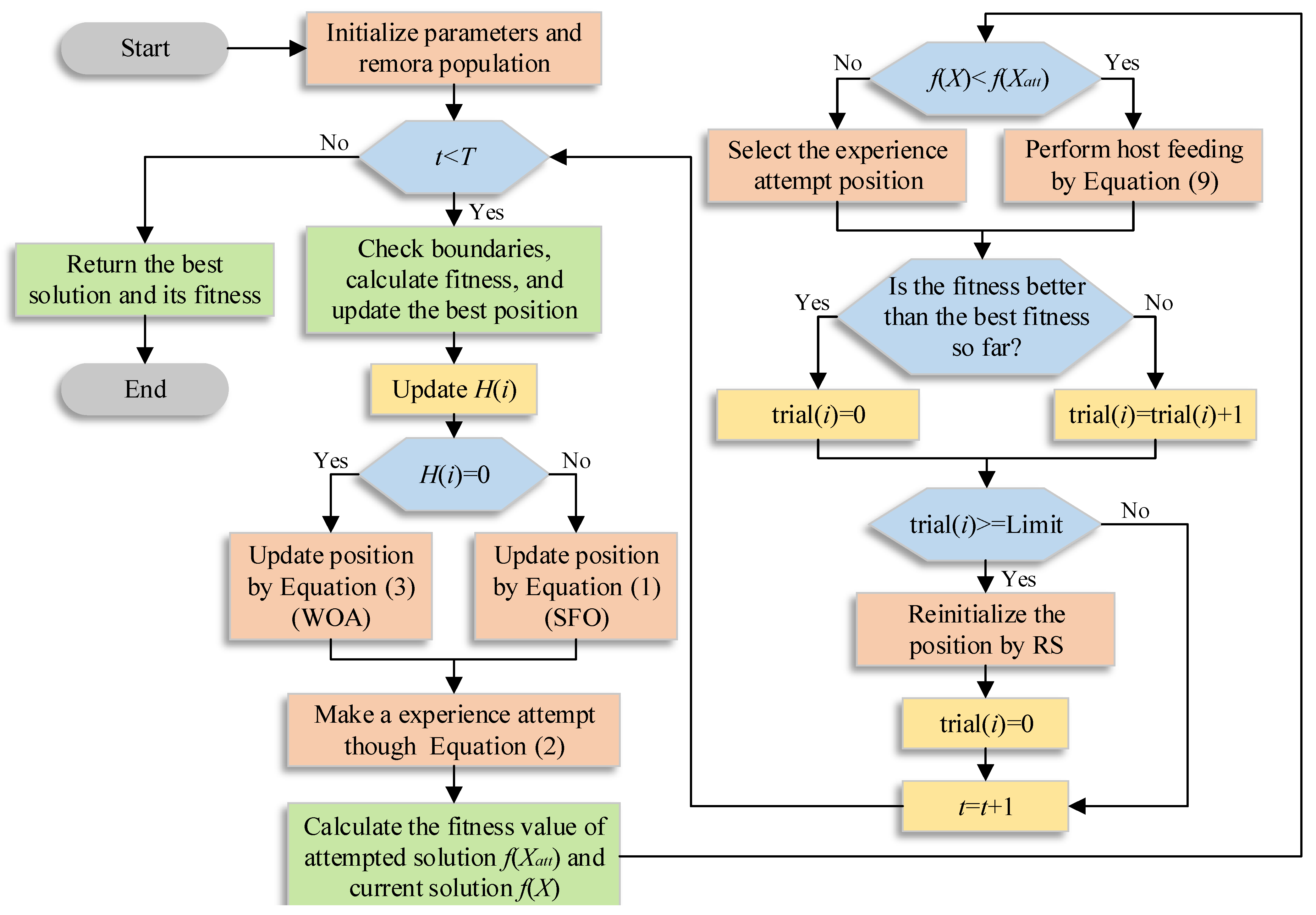
3.4. The Proposed EROA
| Algorithm 2 Pseudo-code of EROA |
|
1: Set initial values of the population size N and the maximum number of iterations T 2: Initialize positions of the population Xi (i = 1, 2, 3, ..., N) 3: Initialize the best solution Xbest and corresponding best fitness f(Xbest) 4: While t < T do 5: Calculate the fitness value of each Remora 6: Check if any search agent goes beyond the search space and amend it 7: Update a, α, and V 8: Update H based on Equation (11) 9: For each Remora indexed by i do 10: If H(i) = 0 then 11: Update the position using Equation (3) 12: Elseif H(i) = 1 then 13: Update the position using Equation (12) 14: End if 15: Make a one-step prediction by Equation (2) 16: Compare fitness values to judge whether host replacement is necessary 17: If the host is not replaced, Equation (7) is used as the host feeding mode for Remora 18: Update trial(i) for remora 19: If trial(i) >= Limit 20: Generate positions using Equations (15) and (17), respectively 21: Compare fitness values to choose the position with better fitness value 22: End if 23: End for 24: End while 25: Return Xbest |
4. Numerical Experiment Results
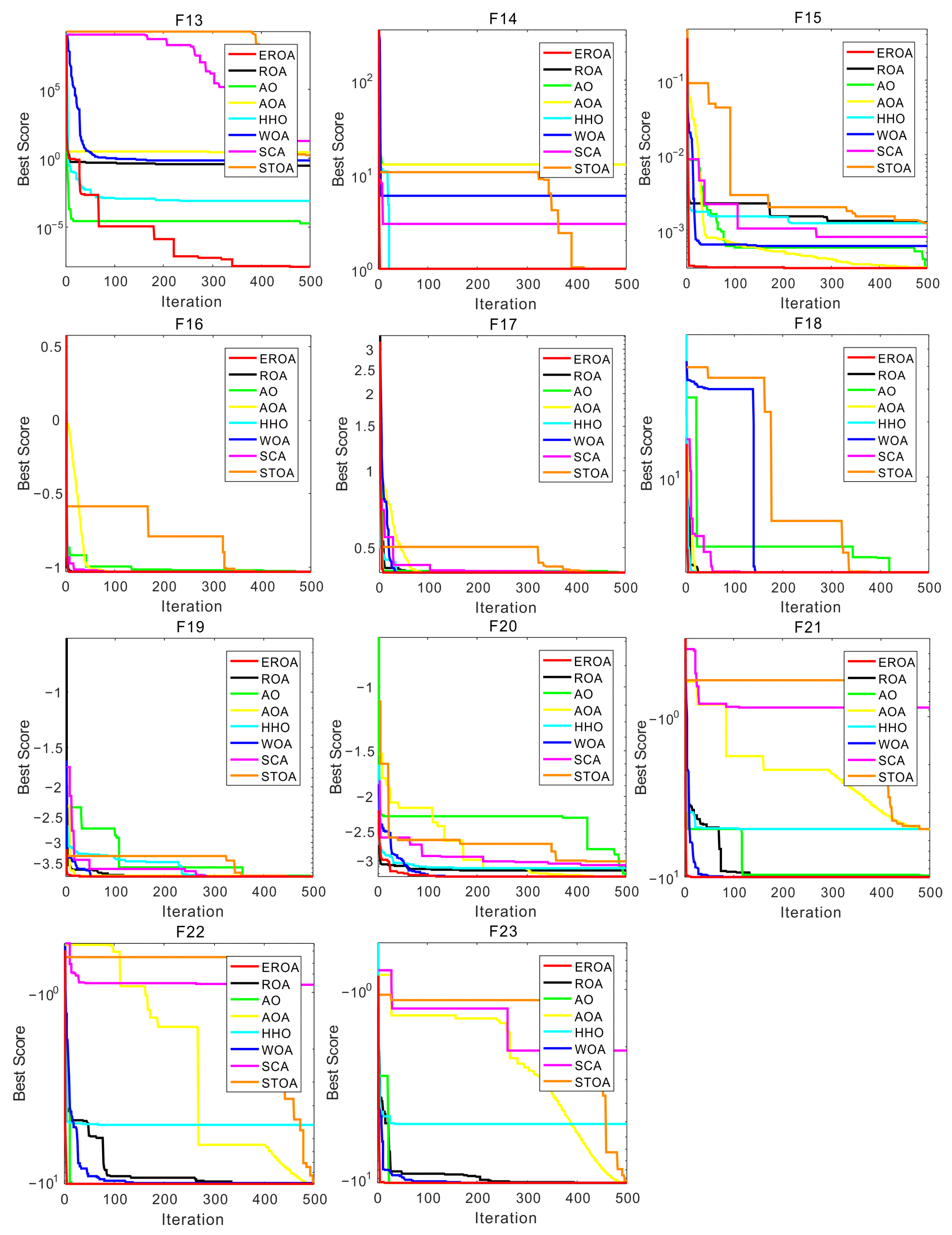
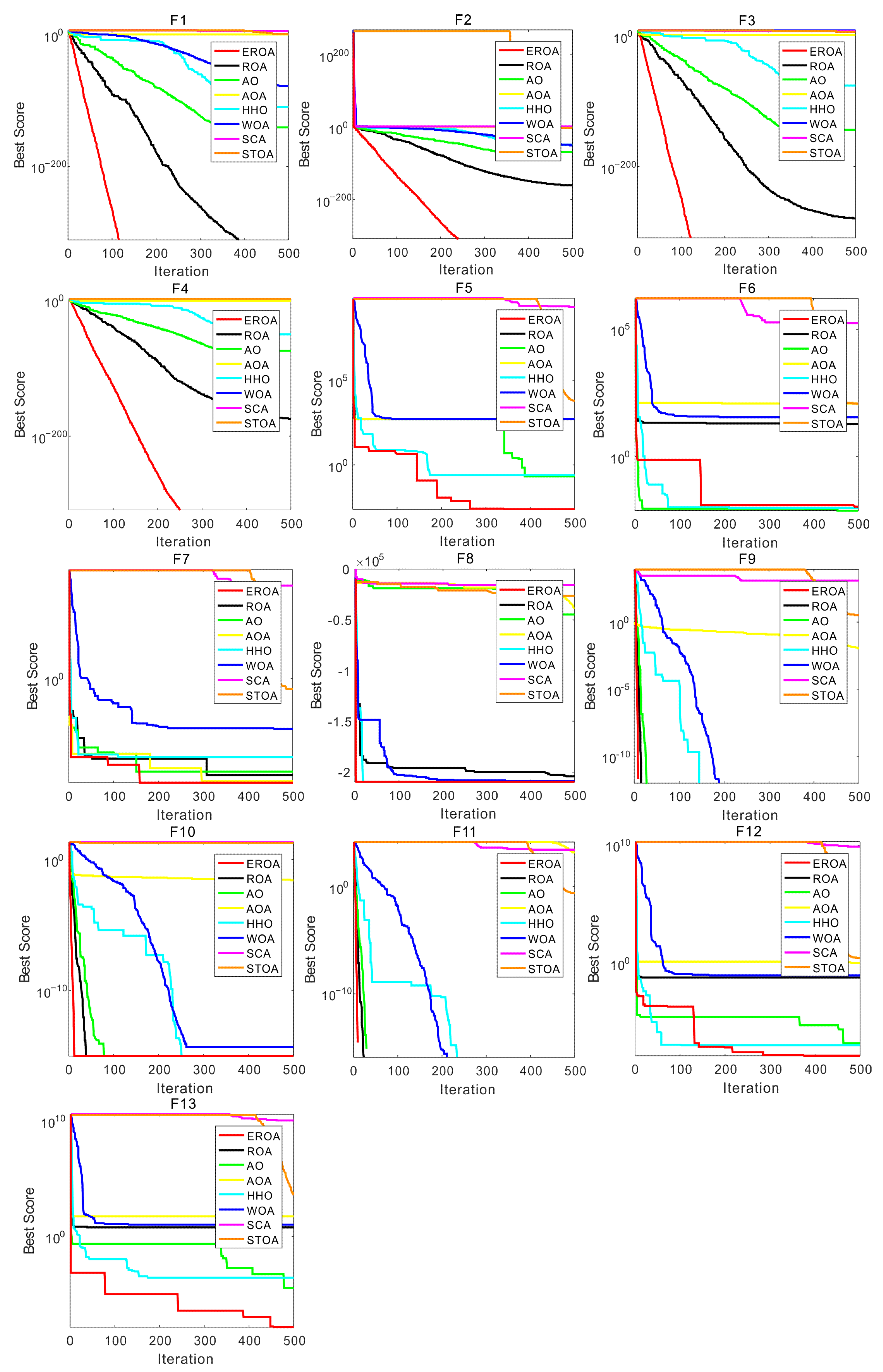
4.1. Experiments on Standard Benchmark Functions
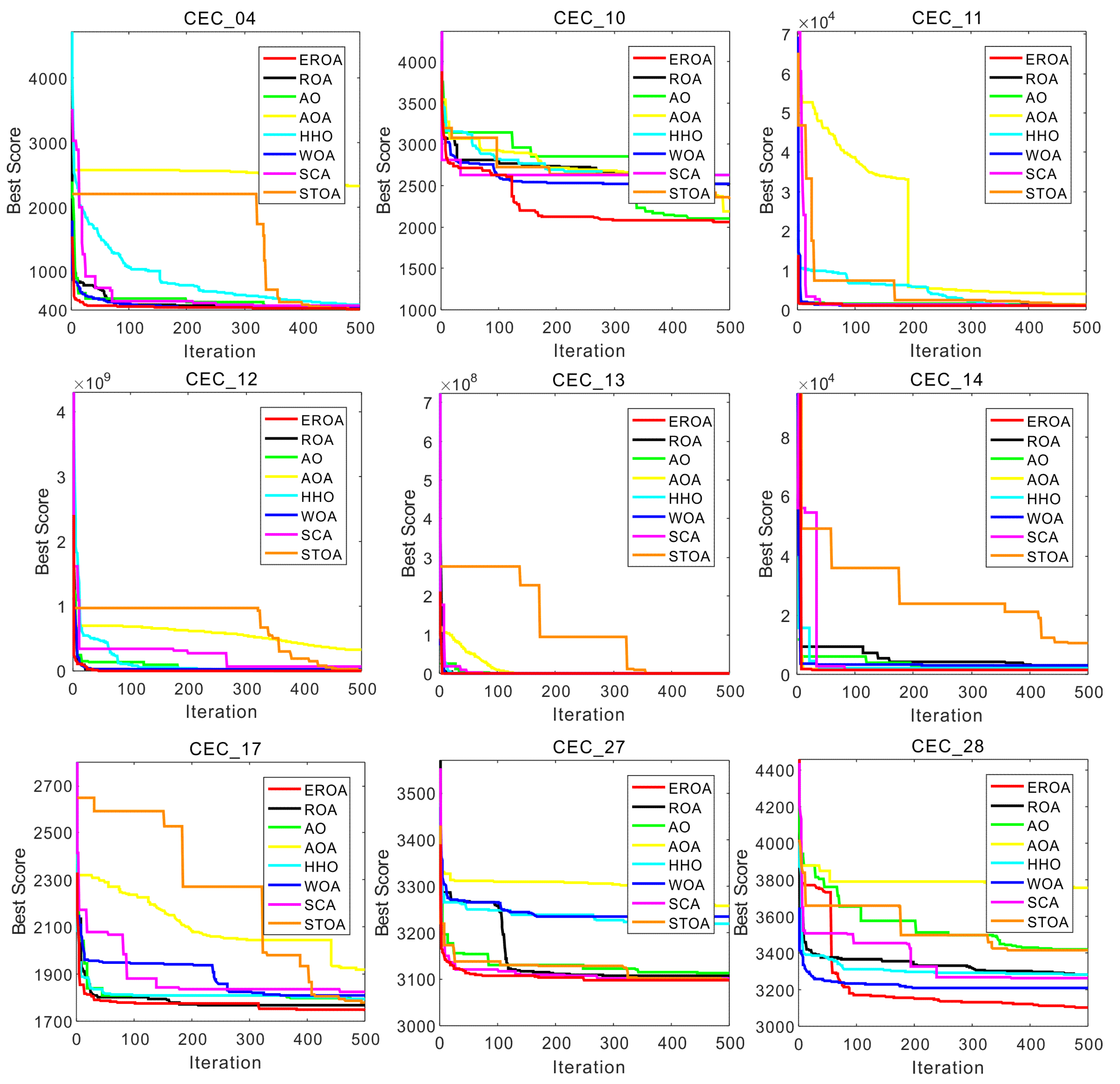
4.2. Experiments on CEC2017 Test Suite
5. Constrained Engineering Design Problems
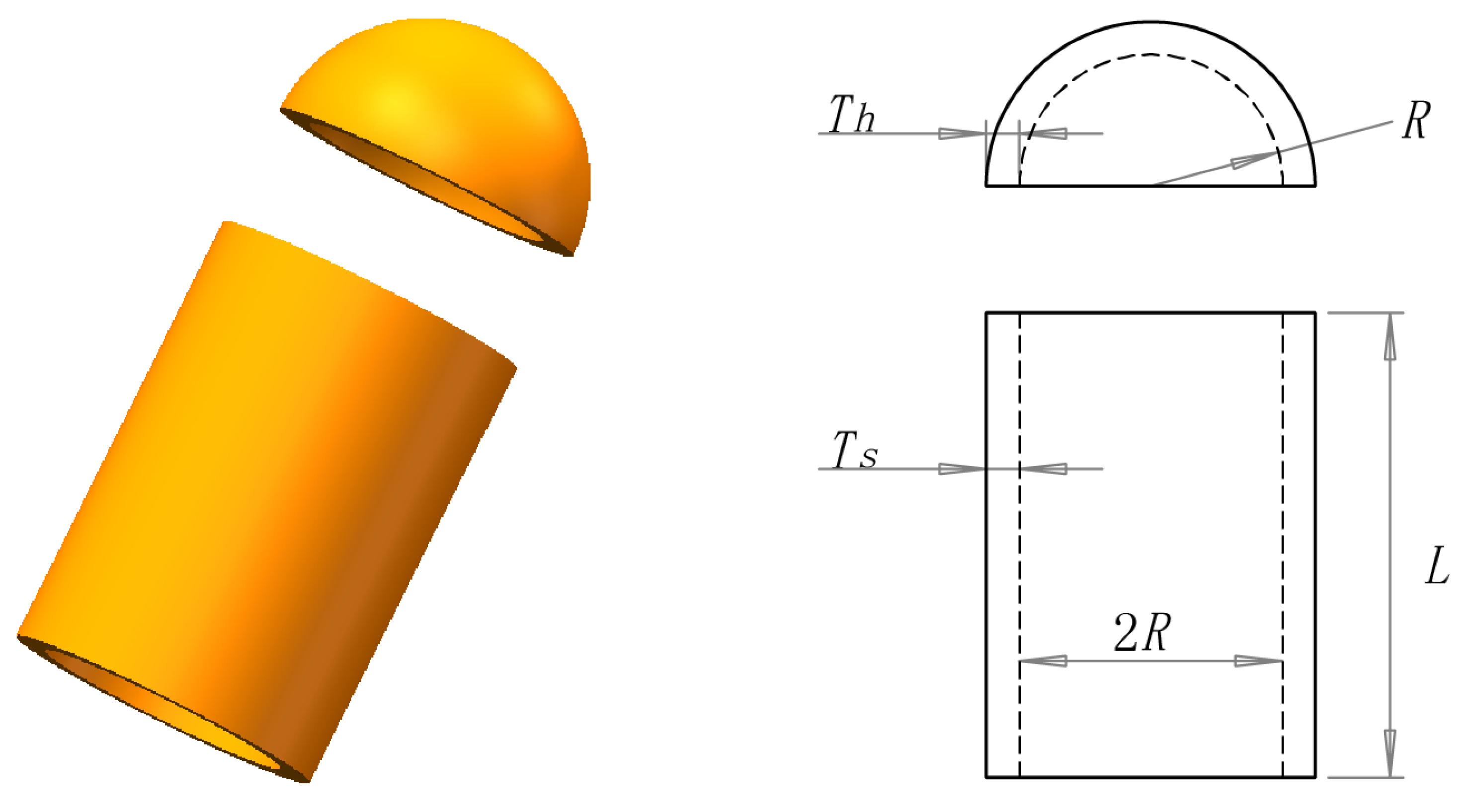
5.1. Pressure Vessel Design Problem
5.2. Speed Reducer Design Problem
5.3. Tension/Compression Spring Design Problem
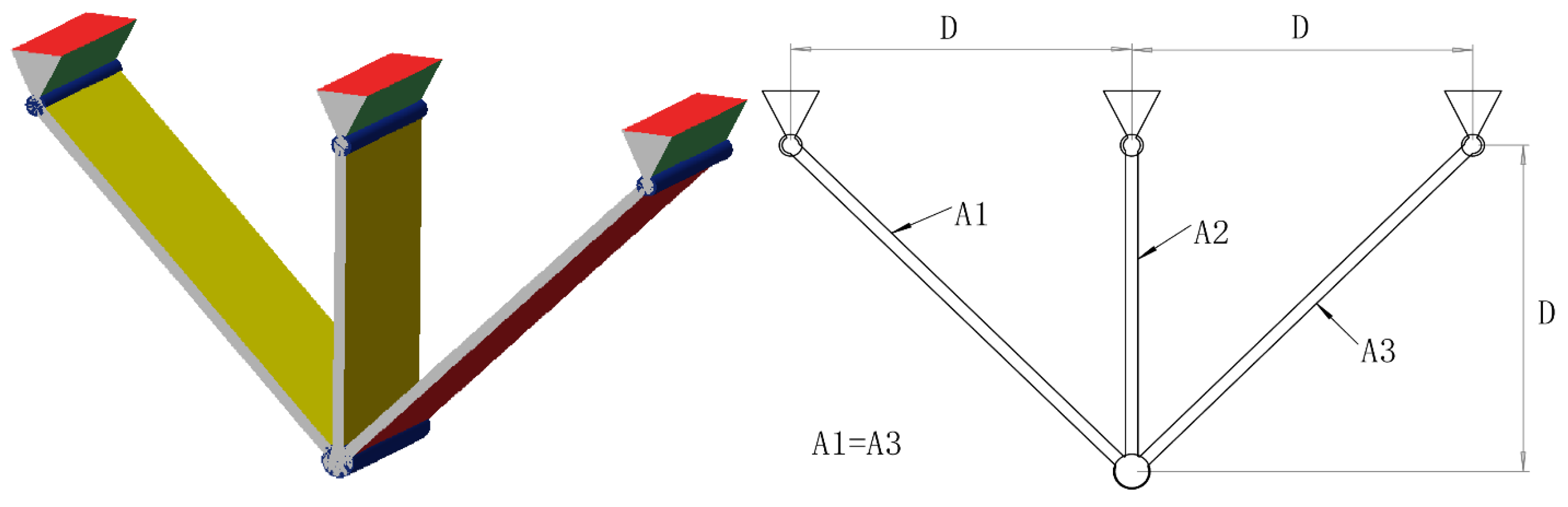
5.4. Three-Bar Truss Design Problem
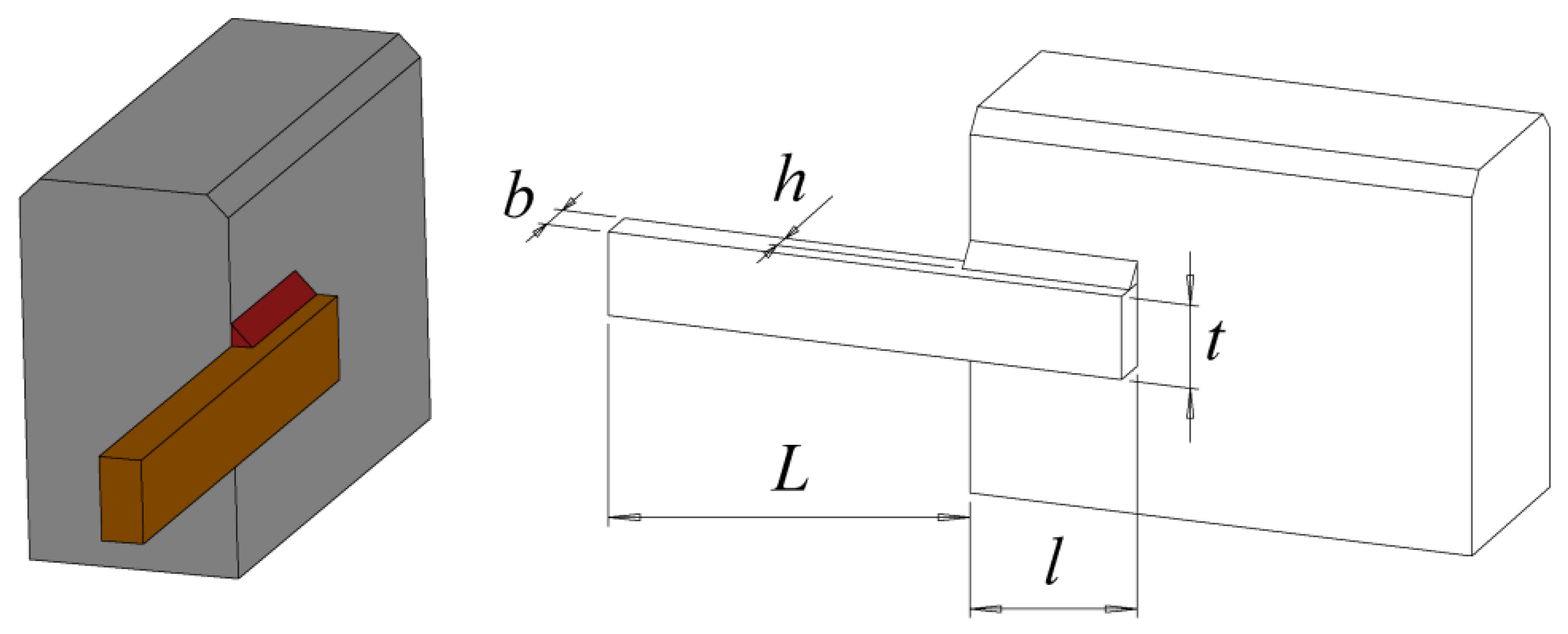
5.5. Welded Beam Design Problem
5.6. Tubular Column Design Problem
5.7. Gear Train Design Problem
6. Conclusions
Author Contributions
Funding
Institutional Review Board Statement
Informed Consent Statement
Data Availability Statement
Acknowledgments
Conflicts of Interest
References
- Yang, X.S. Engineering Optimization: An Introduction with Metaheuristic Applications; John Wiley & Sons: Hoboken, NJ, USA, 2010. [Google Scholar] [CrossRef]
- Abualigah, L.; Gandomi, A.H.; Elaziz, M.A.; Hussien, A.G.; Khasawneh, A.M.; Alshinwan, M.; Houssein, E.H. Nature-inspired optimization algorithms for text document clustering—A comprehensive analysis. Algorithms 2020, 13, 345. [Google Scholar] [CrossRef]
- Hassanien, A.E.; Emary, E. Swarm Intelligence: Principles, Advances, and Applications; CRC Press: Boca Raton, FL, USA, 2018. [Google Scholar]
- Hussien, A.G.; Hassanien, A.E.; Houssein, E.H.; Bhattacharyya, S.; Amin, M. S-shaped binary whale optimization algorithm for feature selection. Recent Trends Signal Image Process. 2019, 727, 79–87. [Google Scholar]
- Fathi, H.; AlSalman, H.; Gumaei, A.; Manhrawy, I.I.; Hussien, A.G.; El-Kafrawy, P. An efficient cancer classification model using microarray and high-dimensional data. Comput. Intell. Neurosci. 2021, 2021, 7231126. [Google Scholar] [CrossRef] [PubMed]
- Hussien, A.G.; Houssein, E.H.; Hassanien, A.E. A binary whale optimization algorithm with hyperbolic tangent fitness function for feature selection. In Proceedings of the 2017 Eighth International Conference on Intelligent Computing and Information Systems (ICICIS), Cairo, Egypt, 5–7 December 2017; pp. 166–172. [Google Scholar] [CrossRef]
- Hussien, A.G.; Amin, M. A self-adaptive harris hawks optimization algorithm with opposition-based learning and chaotic local search strategy for global optimization and feature selection. Int. J. Mach. Learn. Cybern. 2022, 13, 309–336. [Google Scholar] [CrossRef]
- Abdullahi, M.; Ngadi, M.A.; Dishing, S.I.; Ahmad, B.I. An efficient symbiotic organisms search algorithm with chaotic optimization strategy for multi-objective task scheduling problems in cloud computing environment. J. Netw. Comput. Appl. 2019, 133, 60–74. [Google Scholar] [CrossRef]
- Besnassi, M.; Neggaz, N.; Benyettou, A. Face detection based on evolutionary Haar filter. Pattern Anal. Appl. 2020, 23, 309–330. [Google Scholar] [CrossRef]
- Neshat, M.; Mirjalili, S.; Sergiienko, N.Y.; Esmaeilzadeh, S.; Amini, E.; Heydari, A.; Garcia, D.A. Layout optimisation of offshore wave energy converters using a novel multi-swarm cooperative algorithm with backtracking strategy: A case study from coasts of Australia. Energy 2022, 239, 122463. [Google Scholar] [CrossRef]
- Eslami, M.; Neshat, M.; Khalid, S.A. A Novel Hybrid Sine Cosine Algorithm and Pattern Search for Optimal Coordination of Power System Damping Controllers. Sustainability 2022, 14, 541. [Google Scholar] [CrossRef]
- Nadimi-Shahraki, M.H.; Taghian, S.; Mirjalili, S.; Zamani, H.; Bahreininejad, A. GGWO: Gaze cues learning-based grey wolf optimizer and its applications for solving engineering problems. J. Comput. Sci. 2022, 61, 101636. [Google Scholar] [CrossRef]
- Wolpert, D.H.; Macready, W.G. No free lunch theorems for optimization. IEEE Trans. Evol. Comput. 1997, 1, 67–82. [Google Scholar] [CrossRef] [Green Version]
- Hussien, A.G.; Oliva, D.; Houssein, E.H.; Juan, A.A.; Yu, X. Binary whale optimization algorithm for dimensionality reduction. Mathematics 2020, 8, 1821. [Google Scholar] [CrossRef]
- Hussien, A.G.; Hassanien, A.E.; Houssein, E.H. Swarming behaviour of salps algorithm for predicting chemical compound activities. In Proceedings of the 2017 Eighth International Conference on Intelligent Computing and Information Systems (ICICIS), Cairo, Egypt, 5–7 December 2017; pp. 315–320. [Google Scholar]
- Hussien, A.G.; Hassanien, A.E.; Houssein, E.H.; Amin, M.; Azar, A.T. New binary whale optimization algorithm for discrete optimization problems. Eng. Optim. 2020, 52, 945–959. [Google Scholar] [CrossRef]
- Fearn, T. Particle swarm optimisation. NIR News 2014, 25, 27. [Google Scholar] [CrossRef]
- Dorigo, M.; Maniezzo, V.; Colorni, A. Ant system: Optimization by a colony of cooperating agents. IEEE Trans. Syst. Man Cybern. Part B (Cybern.) 1996, 26, 29–41. [Google Scholar] [CrossRef] [Green Version]
- Mirjalili, S.; Mirjalili, S.M.; Lewis, A. Grey wolf optimizer. Adv. Eng. Softw. 2014, 69, 46–61. [Google Scholar] [CrossRef] [Green Version]
- Assiri, A.S.; Hussien, A.G.; Amin, M. Ant lion optimization: Variants, hybrids, and applications. IEEE Access 2020, 8, 77746–77764. [Google Scholar] [CrossRef]
- Mirjalili, S.; Lewis, A. The whale optimization algorithm. Adv. Eng. Softw. 2016, 95, 51–67. [Google Scholar] [CrossRef]
- Faramarzi, A.; Heidarinejad, M.; Mirjalili, S.; Gandomi, A.H. Marine predators algorithm: A nature-inspired metaheuristic. Expert Syst. Appl. 2020, 152, 113377. [Google Scholar] [CrossRef]
- Hussien, A.G. An enhanced opposition-based salp swarm algorithm for global optimization and engineering problems. J. Ambient. Intell. Humaniz. Comput. 2022, 13, 129–150. [Google Scholar] [CrossRef]
- Jia, H.; Peng, X.; Lang, C. Remora optimization algorithm. Expert Syst. Appl. 2021, 185, 115665. [Google Scholar] [CrossRef]
- Heidari, A.A.; Mirjalili, S.; Faris, H.; Aljarah, I.; Mafarja, M.; Chen, H. Harris hawks optimization: Algorithm and applications. Future Gener. Comput. Syst. 2019, 97, 849–872. [Google Scholar] [CrossRef]
- Mostafa, R.R.; Hussien, A.G.; Khan, M.A.; Kadry, S.; Hashim, F. Enhanced coot optimization algorithm for dimensionality reduction. In Proceedings of the 2022 Fifth International Conference of Women in Data Science at Prince Sultan University (WiDS PSU), Riyadh, Saudi Arabia, 28–29 March 2022. [Google Scholar]
- Hussien, A.G.; Amin, M.; Abd El Aziz, M. A comprehensive review of moth-flame optimisation: Variants, hybrids, and applications. J. Exp. Theor. Artif. Intell. 2020, 32, 705–725. [Google Scholar] [CrossRef]
- Cuevas, E.; Cienfuegos, M.; Zaldívar, D.; Perez-Cisneros, M. A swarm optimization algorithm inspired in the behavior of the social-spider. Expert Syst. Appl. 2013, 40, 6374–6384. [Google Scholar] [CrossRef] [Green Version]
- Hashim, F.A.; Hussien, A.G. Snake optimizer: A novel meta-heuristic optimization algorithm. Knowl.-Based Syst. 2022, 242, 108320. [Google Scholar] [CrossRef]
- Hussien, A.G.; Amin, M.; Wang, M.; Liang, G.; Alsanad, A.; Gumaei, A.; Chen, H. Crow search algorithm: Theory, recent advances, and applications. IEEE Access 2020, 8, 173548–173565. [Google Scholar] [CrossRef]
- Dhiman, G.; Kumar, V. Emperor penguin optimizer: A bio-inspired algorithm for engineering problems. Knowl.-Based Syst. 2018, 159, 20–50. [Google Scholar] [CrossRef]
- Hussien, A.G.; Heidari, A.A.; Ye, X.; Liang, G.; Chen, H.; Pan, Z. Boosting whale optimization with evolution strategy and gaussian random walks: An image segmentation method. Eng. Comput. 2022, 1–45. [Google Scholar] [CrossRef]
- Dhiman, G.; Kumar, V. Spotted hyena optimizer: A novel bio-inspired based metaheuristic technique for engineering applications. Adv. Eng. Softw. 2017, 114, 48–70. [Google Scholar] [CrossRef]
- Abualigah, L.; Yousri, D.; Elaziz, M.A.; Ewees, A.A.; Al-qaness, M.A.A.; Gandomi, A.H. Aquila Optimizer: A novel meta-heuristic optimization algorithm. Comput. Ind. Eng. 2021, 157, 107250. [Google Scholar] [CrossRef]
- Kaur, S.; Awasthi, L.K.; Sangal, A.; Dhiman, G. Tunicate swarm algorithm: A new bioinspired based metaheuristic paradigm for global optimization. Eng. Appl. Artif. Intell. 2020, 90, 103541. [Google Scholar] [CrossRef]
- Kirkpatrick, S.; Gelatt, C.D., Jr.; Vecchi, M.P. Optimization by simulated annealing. Science 1983, 220, 671–680. [Google Scholar] [CrossRef] [PubMed]
- Genc¸, H.M.; Eksin, I.; Erol, O.K. Big bang-big crunch optimization algorithm hybridized with local directional moves and application to target motion analysis problem. In Proceedings of the 2010 IEEE International Conference on Systems, Man and Cybernetics, Istanbul, Turkey, 10–13 October 2010; pp. 881–887. [Google Scholar]
- Rashedi, E.; Nezamabadi-Pour, H.; Saryazdi, S. Gsa: A gravitational search algorithm. Inf. Sci. 2009, 179, 2232–2248. [Google Scholar] [CrossRef]
- Abualigah, L.; Elaziz, M.A.; Hussien, A.G.; Alsalibi, B.; Jalali, S.M.J.; Gandomi, A.H. Lightning search algorithm: A comprehensive survey. Appl. Intell. 2021, 51, 2353–2376. [Google Scholar] [CrossRef] [PubMed]
- Hatamlou, A. Black hole: A new heuristic optimization approach for data clustering. Inf. Sci. 2013, 222, 175–184. [Google Scholar] [CrossRef]
- Mirjalili, S. SCA: A Sine Cosine Algorithm for Solving Optimization Problems. Knowl.-Based Syst. 2016, 96, 120–133. [Google Scholar] [CrossRef]
- Kaveh, A.; Khayatazad, M. A new meta-heuristic method: Ray optimization. Comput. Struct. 2012, 112, 283–294. [Google Scholar] [CrossRef]
- Anita; Yadav, A. Aefa: Artificial electric field algorithm for global optimization. Swarm Evol. Comput. 2019, 48, 93–108. [Google Scholar]
- Abualigah, L.; Diabat, A.; Mirjalili, S.; Elaziz, M.A.; Gandomi, A.H. The Arithmetic Optimization Algorithm. Comput. Methods Appl. Mech. Eng. 2021, 376, 113609. [Google Scholar] [CrossRef]
- Mirjalili, S.; Mirjalili, S.M.; Hatamlou, A. Multi-verse optimizer: A nature-inspired algorithm for global optimization. Neural Comput. Appl. 2015, 27, 495–513. [Google Scholar] [CrossRef]
- Hashim, F.A.; Houssein, E.H.; Mabrouk, M.S.; Al-Atabany, W.; Mirjalili, S. Henry gas solubility optimization: A novel physics-based algorithm. Future Gener. Comput. Syst. 2019, 101, 646–667. [Google Scholar] [CrossRef]
- Holland, J.H. Genetic algorithms. Sci. Am. 1992, 267, 66–73. [Google Scholar] [CrossRef]
- Sinha, N.; Chakrabarti, R.; Chattopadhyay, P. Evolutionary programming techniques for economic load dispatch. IEEE Trans. Evol. Comput. 2003, 7, 83–94. [Google Scholar] [CrossRef]
- Simon, D. Biogeography-based optimization. IEEE Trans. Evol. Comput. 2008, 12, 702–713. [Google Scholar] [CrossRef] [Green Version]
- Moscato, P.; Cotta, C.; Mendes, A. Memetic algorithms. In New Optimization Techniques in Engineering; Springer: Berlin/Heidelberg, Germany, 2004; pp. 53–85. [Google Scholar]
- Passino, K.M. Bacterial foraging optimization. Int. J. Swarm Intell. Res. (IJSIR) 2010, 1, 1–16. [Google Scholar] [CrossRef]
- Uymaz, S.A.; Tezel, G.; Yel, E. Artificial algae algorithm (aaa) for nonlinear global optimization. Appl. Soft Comput. 2015, 31, 153–171. [Google Scholar] [CrossRef]
- Meng, Z.; Pan, J.S. Monkey king evolution: A new memetic evolutionary algorithm and its application in vehicle fuel consumption optimization. Knowl.-Based Syst. 2016, 97, 144–157. [Google Scholar] [CrossRef]
- Zheng, R.; Jia, H.; Abualigah, L.; Wang, S.; Wu, D. An improved remora optimization algorithm with autonomous foraging mechanism for global optimization problems. Math. Biosci. Eng. 2022, 19, 3994–4037. [Google Scholar] [CrossRef]
- Liu, Q.; Li, N.; Jia, H.; Qi, Q.; Abualigah, L. Modified remora optimization algorithm for global optimization and multilevel thresholding image segmentation. Mathematics 2022, 10, 1014. [Google Scholar] [CrossRef]
- Vinayaki, V.D.; Kalaiselvi, R. Multithreshold image segmentation technique using remora optimization algorithm for diabetic retinopathy detection from fundus images. Neural Process. Lett. 2022, 1–22. [Google Scholar] [CrossRef]
- Shadravan, S.; Naji, H.R.; Bardsiri, V.K. The Sailfish Optimizer: A novel nature-inspired metaheuristic algorithm for solving constrained engineering optimization problems. Eng. Appl. Artif. Intell. 2019, 80, 20–34. [Google Scholar] [CrossRef]
- Zhang, H.; Wang, Z.; Chen, W.; Heidari, A.A.; Wang, M.; Zhao, X.; Liang, G.; Chen, H.; Zhang, X. Ensemble mutation-driven salp swarm algorithm with restart mechanism: Framework and fundamental analysis. Expert Syst. Appl. 2021, 165, 113897. [Google Scholar] [CrossRef]
- Long, W.; Jiao, J.; Liang, X.; Cai, S.; Xu, M. A Random Opposition-Based Learning Grey Wolf Optimizer. IEEE Access 2019, 7, 113810–113825. [Google Scholar] [CrossRef]
- Dhiman, G.; Kaur, A. STOA: A bio-inspired based optimization algorithm for industrial engineering problems. Eng. Appl. Artif. Intell. 2019, 82, 148–174. [Google Scholar] [CrossRef]
- Li, S.M.; Chen, H.L.; Wang, M.J.; Heidari, A.A.; Mirjalili, S. Slime mould algorithm: A new method for stochastic optimization. Future Gener. Comput. Syst. 2020, 111, 300–323. [Google Scholar] [CrossRef]
- Rechenberg, I. Evolutionsstrategien. In Simulationsmethoden in der Medizin und Biologie; Springer: Berlin/Heidelberg, Germany, 1978; Volume 8, pp. 83–114. [Google Scholar]
- He, Q.; Wang, L. An effective co-evolutionary particle swarm optimization for constrained engineering design problems. Eng. Appl. Artif. Intell. 2007, 20, 89–99. [Google Scholar] [CrossRef]
- Geem, Z.W.; Kim, J.H.; Loganathan, G.V. A new heuristic optimization algorithm: Harmony search. Simulation 2001, 76, 60–68. [Google Scholar] [CrossRef]
- Lu, S.; Kim, H.M. A regularized inexact penalty decomposition algorithm for multidisciplinary design optimization problems with complementarity constraints. J. Mech. Des. 2010, 132, 041005. [Google Scholar] [CrossRef] [Green Version]
- Wu, D.; Wang, S.; Liu, Q.; Abualigah, L.; Jia, H. An Improved Teaching-Learning-Based Optimization Algorithm with Reinforcement Learning Strategy for Solving Optimization Problems. Comput. Intell. Neurosci. 2022, 2022, 1535957. [Google Scholar] [CrossRef]
- Saremi, S.; Mirjalili, S.; Lewis, A. Grasshopper optimisation algorithm: Theory and application. Adv. Eng. Softw. 2017, 105, 30–47. [Google Scholar] [CrossRef] [Green Version]
- Wang, S.; Jia, H.; Abualigah, L.; Liu, Q.; Zheng, R. An Improved Hybrid Aquila Optimizer and Harris Hawks Algorithm for Solving Industrial Engineering Optimization Problems. Processes 2021, 9, 1551. [Google Scholar] [CrossRef]
- Zheng, R.; Hussien, A.G.; Jia, H.; Abualigah, L.; Wang, S.; Wu, D. An Improved Wild Horse Optimizer for Solving Optimization Problems. Mathematics 2022, 10, 1311. [Google Scholar] [CrossRef]
- Gandomi, A.H.; Yang, X.S.; Alavi, A.H. Cuckoo search algorithm: A metaheuristic approach to solve structural optimization problems. Eng. Comput. 2013, 29, 17–35. [Google Scholar] [CrossRef]
- Wang, S.; Sun, K.; Zhang, W.; Jia, H. Multilevel thresholding using a modified ant lion optimizer with opposition-based learning for color image segmentation. Math. Biosci. Eng. 2021, 18, 3092–3143. [Google Scholar] [CrossRef] [PubMed]
- Sharma, T.K.; Pant, M.; Singh, V. Improved local search in artificial bee colony using golden section search. arXiv 2012, arXiv:1210.6128. [Google Scholar]
- Sadollah, A.; Bahreininejad, A.; Eskandar, H.; Hamdi, M. Mine blast algorithm: A new population based algorithm for solving constrained engineering optimization problems. Appl. Soft Comput. 2013, 13, 2592–2612. [Google Scholar] [CrossRef]


| Algorithm | Parameters |
|---|---|
| EROA | C = 0.1; Limit = log(t) |
| ROA | C = 0.1 |
| AO | U = 0.00565; r1 = 10; ω = 0.005; α = 0.1; δ = 0.1; G1∈[−1, 1]; G2 = [2, 0] |
| AOA | α = 5; μ = 0.5; |
| HHO | q∈[0, 1]; r∈[0, 1]; E0∈[−1, 1]; E1 = [2, 0]; E∈[−2, 2]; |
| WOA | a1 = [2, 0]; a2 = [−1, −2]; b = 1 |
| STOA | Cf = 2; u = 1; v = 1 |
| Fun. | D | Range | fmin |
|---|---|---|---|
| 30/100/500 | [−100, 100] | 0 | |
| 30/100/500 | [−10, 10] | 0 | |
| 30/100/500 | [−100, 100] | 0 | |
| 30/100/500 | [−100, 100] | 0 | |
| 30/100/500 | [−30, 30] | 0 | |
| 30/100/500 | [−100, 100] | 0 | |
| 30/100/500 | [−1.28, 1.28] | 0 |
| Fun. | D | Range | fmin |
|---|---|---|---|
| 30/100/500 | [−500, 500] | −418.9829 × D | |
| 30/100/500 | [−5.12, 5.12] | 0 | |
| 30/100/500 | [−32, 32] | 0 | |
| 30/100/500 | [−600, 600] | 0 | |
| 30/100/500 | [−50, 50] | 0 | |
| 30/100/500 | [−50, 50] | 0 |
| Fun. | D | Range | fmin |
|---|---|---|---|
| 2 | [−65, 65] | 1 | |
| 4 | [−5, 5] | 0.00030 | |
| 2 | [−5, 5] | −1.0316 | |
| 2 | [−5, 5] | 0.398 | |
| 2 | [−2, 2] | 3 | |
| 3 | [−1, 2] | −3.86 | |
| 6 | [0, 1] | −3.32 | |
| 4 | [0, 10] | −10.1532 | |
| 4 | [0, 10] | −10.4028 | |
| 4 | [0, 10] | −10.5363 |
| F | D | EROA | ROA | AO | AOA | HHO | WOA | SCA | STOA | |
|---|---|---|---|---|---|---|---|---|---|---|
| F1 | 30 | Avg | 0 | 7.33 × 10−314 | 2.73 × 10−102 | 4.83 × 10⁻⁶ | 2.34 × 10−95 | 4.15 × 10−72 | 9.65 | 5.81 × 10⁻⁷ |
| Std | 0 | 0 | 1.49 × 10−101 | 1.81 × 10⁻⁶ | 1.26 × 10−94 | 2.25 × 10−71 | 1.71 × 101 | 1.24 × 10⁻⁶ | ||
| 100 | Avg | 0 | 0 | 1.47 × 10−98 | 9.93 × 10⁻⁴ | 5.55 × 10−93 | 9.06 × 10−72 | 1.08 × 10⁴ | 9.12 × 10⁻³ | |
| Std | 0 | 0 | 8.02 × 10−98 | 2.80 × 10⁻⁴ | 2.05 × 10−92 | 2.16 × 10−71 | 7.78 × 10³ | 1.22 × 10⁻² | ||
| 500 | Avg | 0 | 0 | 7.28 × 10−102 | 5.24 × 10⁻¹ | 9.52 × 10−97 | 4.70 × 10−70 | 2.17 × 10⁵ | 9.52 | |
| Std | 0 | 0 | 3.86 × 10−101 | 3.36 × 10⁻² | 3.92 × 10−96 | 1.35 × 10−69 | 7.89 × 10⁴ | 9.27 | ||
| F2 | 30 | Avg | 0 | 1.16 × 10−165 | 4.63 × 10−64 | 1.50 × 10⁻³ | 9.36 × 10−51 | 6.83 × 10−50 | 1.69 × 10⁻² | 1.01 × 10⁻⁵ |
| Std | 0 | 0 | 2.32 × 10−63 | 1.92 × 10⁻³ | 3.73 × 10−50 | 3.45 × 10−49 | 2.25 × 10⁻² | 1.06 × 10⁻⁵ | ||
| 100 | Avg | 0 | 7.40 × 10−162 | 5.90 × 10−55 | 1.85 × 10⁻² | 2.07 × 10−50 | 1.24 × 10−49 | 1.27E × 101 | 2.65 × 10⁻³ | |
| Std | 0 | 4.04 × 10−161 | 2.61 × 10−54 | 2.34 × 10⁻³ | 8.48 × 10−50 | 5.08 × 10−49 | 1.03 × 101 | 2.05 × 10⁻³ | ||
| 500 | Avg | 0 | 9.24 × 10−160 | 1.46 × 10−57 | 5.24 × 10⁻¹ | 1.17 × 10−48 | 1.22 × 10−47 | 1.11 × 10² | 9.34 × 10⁻² | |
| Std | 0 | 3.95 × 10−159 | 8.01 × 10−57 | 9.93 × 10⁻² | 5.95 × 10−48 | 6.19 × 10−47 | 7.32 × 101 | 6.76 × 10⁻² | ||
| F3 | 30 | Avg | 0 | 1.68 × 10−289 | 9.44 × 10−111 | 9.51 × 10⁻⁴ | 2.69 × 10−67 | 4.09 × 10⁴ | 1.11 × 10⁴ | 7.91 × 10⁻² |
| Std | 0 | 0 | 3.78 × 10−110 | 7.68 × 10⁻⁴ | 1.47 × 10−66 | 1.39 × 10⁴ | 7.68 × 10³ | 9.41 × 10⁻² | ||
| 100 | Avg | 0 | 3.32 × 10−276 | 5.31 × 10−100 | 1.30 × 10⁻¹ | 3.89 × 10−62 | 1.09 × 10⁶ | 2.49 × 10⁵ | 2.12 × 10³ | |
| Std | 0 | 0 | 2.91 × 10−99 | 3.20 × 10⁻² | 2.11 × 10−61 | 3.07 × 10⁵ | 4.85 × 10⁴ | 3.24 × 10³ | ||
| 500 | Avg | 0 | 1.09 × 10−253 | 3.30 × 10−104 | 6.91 | 4.61 × 10−39 | 3.38 × 10⁷ | 7.15 × 10⁶ | 5.89 × 10⁵ | |
| Std | 0 | 0 | 1.02 × 10−103 | 1.24 | 2.53 × 10−38 | 1.05 × 10⁷ | 1.79 × 10⁶ | 2.47 × 10⁵ | ||
| F4 | 30 | Avg | 0 | 3.71 × 10−156 | 6.47 × 10−53 | 1.67 × 10⁻² | 3.18 × 10−48 | 5.54 × 101 | 3.20 × 101 | 5.18 × 10⁻² |
| Std | 0 | 2.03 × 10−155 | 2.57 × 10−52 | 1.24 × 10⁻² | 1.71 × 10−47 | 2.37 × 101 | 1.33 × 101 | 5.14 × 10⁻² | ||
| 100 | Avg | 0 | 5.19 × 10−156 | 1.20 × 10−55 | 5.57 × 10⁻³ | 5.67 × 10−48 | 7.59 × 101 | 8.97 × 101 | 7.04 × 101 | |
| Std | 0 | 2.83 × 10−155 | 6.59 × 10−55 | 5.81 × 10⁻³ | 2.84 × 10−47 | 2.24 × 101 | 3.28 | 1.61 × 101 | ||
| 500 | Avg | 0 | 3.95 × 10−152 | 5.72 × 10−54 | 1.21 × 10⁻¹ | 4.10 × 10−49 | 8.22 × 101 | 9.91 × 101 | 9.87 × 101 | |
| Std | 0 | 2.16 × 10−151 | 2.85 × 10−53 | 9.18 × 10⁻³ | 1.93 × 10−48 | 2.13 × 101 | 3.52 × 10⁻¹ | 5.42 × 10⁻¹ | ||
| F5 | 30 | Avg | 6.52 × 10⁻² | 2.71 × 101 | 9.40 × 10⁻³ | 2.79 × 101 | 1.28 × 10⁻² | 2.79 × 101 | 7.71 × 10⁴ | 2.84 × 101 |
| Std | 1.58 × 10⁻² | 4.46 × 10⁻¹ | 2.72 × 10⁻² | 2.37 × 10⁻¹ | 1.39 × 10⁻² | 4.94 × 10⁻¹ | 2.34 × 10⁵ | 5.01 × 10⁻¹ | ||
| 100 | Avg | 2.73 × 10⁻¹ | 9.76 × 101 | 2.29 × 10⁻² | 9.82 × 101 | 3.42 × 10⁻² | 9.81 × 101 | 1.08 × 10⁸ | 1.06 × 10² | |
| Std | 5.56 × 10⁻¹ | 4.54 × 10⁻¹ | 3.13 × 10⁻² | 5.63 × 10⁻² | 4.13 × 10⁻² | 2.42 × 10⁻¹ | 3.96 × 10⁷ | 6.54 | ||
| 500 | Avg | 8.84 × 10⁻¹ | 4.95 × 10² | 1.00 × 10⁻¹ | 4.99 × 10² | 2.39 × 10⁻¹ | 4.96 × 10² | 2.06 × 10⁹ | 1.23 × 10⁴ | |
| Std | 1.97 | 3.06 × 10⁻¹ | 1.26 × 10⁻¹ | 1.37 × 10⁻¹ | 4.50 × 10⁻¹ | 4.25 × 10⁻¹ | 4.56 × 10⁸ | 1.07 × 10⁴ | ||
| F6 | 30 | Avg | 4.53 × 10⁻⁴ | 1.05 × 10⁻¹ | 1.52 × 10⁻⁴ | 3.02 | 9.07 × 10⁻⁵ | 4.33 × 10⁻¹ | 2.06 × 101 | 2.59 |
| Std | 2.66 × 10⁻⁴ | 9.54 × 10⁻² | 4.51 × 10⁻⁴ | 2.46 × 10⁻¹ | 1.74 × 10⁻⁴ | 2.21 × 10⁻¹ | 3.95 × 101 | 5.09 × 10⁻¹ | ||
| 100 | Avg | 1.00 × 10⁻² | 1.84 | 9.23 × 10⁻⁴ | 1.59 × 101 | 4.92 × 10⁻⁴ | 4.33 | 1.37 × 10⁴ | 1.77 × 101 | |
| Std | 1.50 × 10⁻² | 5.34 × 10⁻¹ | 2.94 × 10⁻³ | 7.25 × 10⁻¹ | 5.53 × 10⁻⁴ | 1.21 | 8.42 × 10³ | 7.95 × 10⁻¹ | ||
| 500 | Avg | 9.47 × 10⁻² | 1.56 × 101 | 6.07 × 10⁻⁴ | 1.12 × 10² | 1.82 × 10⁻³ | 3.31 × 101 | 2.11 × 10⁵ | 1.24 × 10² | |
| Std | 1.28 × 10⁻¹ | 4.43 | 8.88 × 10⁻⁴ | 1.64 | 2.10 × 10⁻³ | 9.98 | 6.42 × 10⁴ | 6.66 | ||
| F7 | 30 | Avg | 8.37 × 10⁻⁵ | 1.36 × 10⁻⁴ | 1.01 × 10⁻⁴ | 9.06 × 10⁻⁵ | 1.57 × 10⁻⁴ | 4.18 × 10⁻³ | 9.69 × 10⁻² | 5.85 × 10⁻³ |
| Std | 5.99 × 10⁻⁵ | 1.20 × 10⁻⁴ | 6.70 × 10⁻⁵ | 8.11 × 10⁻⁵ | 1.32 × 10⁻⁴ | 4.43 × 10⁻³ | 1.13 × 10⁻¹ | 2.83 × 10⁻³ | ||
| 100 | Avg | 1.11 × 10⁻⁴ | 1.57 × 10⁻⁴ | 1.22 × 10⁻⁴ | 7.75 × 10⁻⁵ | 1.57 × 10⁻⁴ | 4.78 × 10⁻³ | 1.66 × 10² | 2.58 × 10⁻² | |
| Std | 1.02 × 10⁻⁴ | 2.34 × 10⁻⁴ | 1.30 × 10⁻⁴ | 7.26 × 10⁻⁵ | 1.61 × 10⁻⁴ | 4.32 × 10⁻³ | 9.84 × 101 | 1.10 × 10⁻² | ||
| 500 | Avg | 7.39 × 10⁻⁵ | 1.47 × 10⁻⁴ | 6.99 × 10⁻⁵ | 6.12 × 10⁻⁵ | 1.77 × 10⁻⁴ | 4.38 × 10⁻³ | 1.44 × 10⁴ | 4.94 × 10⁻¹ | |
| Std | 7.05 × 10⁻⁵ | 1.24 × 10⁻⁴ | 5.04 × 10⁻⁵ | 6.66 × 10⁻⁵ | 1.94 × 10⁻⁴ | 5.40 × 10⁻³ | 4.06 × 10³ | 2.40 × 10⁻¹ | ||
| F8 | 30 | Avg | −1.26 × 10⁴ | −1.23 × 10⁴ | −7.48 × 10³ | −5.34 × 10³ | −1.26 × 10⁴ | −1.03 × 10⁴ | −3.91 × 10³ | −5.12 × 10³ |
| Std | 2.20 × 10⁻² | 7.21 × 10² | 3.74 × 10³ | 3.69 × 10² | 9.54 × 101 | 1.74 × 10³ | 3.78 × 10² | 4.44 × 10² | ||
| 100 | Avg | −4.19 × 10⁴ | −4.14 × 10⁴ | −1.09 × 10⁴ | −1.40 × 10⁴ | −4.19 × 10⁴ | −3.52 × 10⁴ | −6.83 × 10³ | −1.10 × 10⁴ | |
| Std | 1.79 × 10⁻¹ | 1.45 × 10³ | 6.20 × 10³ | 7.36 × 10² | 3.35 | 6.14 × 10³ | 5.65 × 10² | 1.51 × 10³ | ||
| 500 | Avg | −2.09 × 10⁵ | −2.07 × 10⁵ | −3.90 × 10⁴ | −3.82 × 10⁴ | −2.09 × 10⁵ | −1.66 × 10⁵ | −1.55 × 10⁴ | −2.50 × 10⁴ | |
| Std | 3.46 | 5.11 × 10³ | 1.04 × 10⁴ | 1.54 × 10³ | 2.02 × 10³ | 2.86 × 10⁴ | 1.28 × 10³ | 3.26 × 10³ | ||
| F9 | 30 | Avg | 0 | 0 | 0 | 1.20 × 10⁻⁶ | 0 | 1.89 × 10⁻¹⁵ | 4.33 × 101 | 1.26 × 101 |
| Std | 0 | 0 | 0 | 1.08 × 10⁻⁶ | 0 | 1.04 × 10⁻¹⁴ | 3.79 × 101 | 1.67 × 101 | ||
| 100 | Avg | 0 | 0 | 0 | 1.85 × 10⁻⁴ | 0 | 0 | 3.23 × 10² | 1.26 × 101 | |
| Std | 0 | 0 | 0 | 3.93 × 10⁻⁵ | 0 | 0 | 1.08 × 10² | 8.97 | ||
| 500 | Avg | 0 | 0 | 3.03 × 10⁻¹⁴ | 1.11 × 10⁻² | 0 | 0 | 1.44 × 10³ | 2.76 × 101 | |
| Std | 0 | 0 | 1.66 × 10⁻¹³ | 7.83 × 10⁻⁴ | 0 | 0 | 5.64 × 10² | 1.88 × 101 | ||
| F10 | 30 | Avg | 8.88 × 10⁻¹⁶ | 8.88 × 10⁻¹⁶ | 8.88 × 10⁻¹⁶ | 4.15 × 10⁻⁴ | 8.88 × 10⁻¹⁶ | 4.91 × 10⁻¹⁵ | 1.21 × 101 | 1.99 × 101 |
| Std | 0 | 0 | 0 | 1.78 × 10⁻⁴ | 0 | 2.23 × 10⁻¹⁵ | 9.25 | 1.49 × 10⁻³ | ||
| 100 | Avg | 8.88 × 10⁻¹⁶ | 8.88 × 10⁻¹⁶ | 8.88 × 10⁻¹⁶ | 3.42 × 10⁻³ | 8.88 × 10⁻¹⁶ | 4.91 × 10⁻¹⁵ | 1.81 × 101 | 2.00 × 101 | |
| Std | 0 | 0 | 0 | 3.76 × 10⁻⁴ | 0 | 3.06 × 10⁻¹⁵ | 4.95 | 3.43 × 10⁻⁴ | ||
| 500 | Avg | 8.88 × 10⁻¹⁶ | 8.88 × 10⁻¹⁶ | 8.88 × 10⁻¹⁶ | 2.67 × 10⁻² | 8.88 × 10⁻¹⁶ | 3.26 × 10⁻¹⁵ | 1.93E × 101 | 2.00 × 101 | |
| Std | 0 | 0 | 0 | 9.11 × 10⁻⁴ | 0 | 2.35 × 10⁻¹⁵ | 3.32 | 6.17 × 10⁻⁵ | ||
| F11 | 30 | Avg | 0 | 0 | 0 | 1.09 × 10⁻³ | 0 | 2.49 × 10⁻² | 8.85 × 10⁻¹ | 1.81 × 10⁻² |
| Std | 0 | 0 | 0 | 4.17 × 10⁻³ | 0 | 7.26 × 10⁻² | 3.10 × 10⁻¹ | 2.16 × 10⁻² | ||
| 100 | Avg | 0 | 0 | 0 | 1.42 × 10⁻¹ | 0 | 0 | 8.53 × 101 | 4.58 × 10⁻² | |
| Std | 0 | 0 | 0 | 1.61 × 10⁻¹ | 0 | 0 | 6.15 × 101 | 5.97 × 10⁻² | ||
| 500 | Avg | 0 | 0 | 0 | 1.35 × 10³ | 0 | 0 | 1.85 × 10³ | 6.45 × 10⁻¹ | |
| Std | 0 | 0 | 0 | 5.15 × 10² | 0 | 0 | 7.02 × 10² | 2.99 × 10⁻¹ | ||
| F12 | 30 | Avg | 1.35 × 10⁻⁵ | 9.35 × 10⁻³ | 6.63 × 10⁻⁶ | 7.42 × 10⁻¹ | 1.55 × 10⁻⁵ | 1.66 × 10⁻¹ | 1.32 × 10⁵ | 2.62 × 10⁻¹ |
| Std | 1.23 × 10⁻⁵ | 6.03 × 10⁻³ | 1.26 × 10⁻⁵ | 2.08 × 10⁻² | 1.93 × 10⁻⁵ | 7.90 × 10⁻¹ | 5.71 × 10⁵ | 1.71 × 10⁻¹ | ||
| 100 | Avg | 6.55 × 10⁻⁶ | 2.20 × 10⁻² | 1.07 × 10⁻⁶ | 9.10 × 10⁻¹ | 2.57 × 10⁻⁵ | 5.52 × 10⁻² | 3.21 × 10⁸ | 7.79 × 10⁻¹ | |
| Std | 9.69 × 10⁻⁶ | 1.10 × 10⁻² | 2.81 × 10⁻⁶ | 6.55 × 10⁻² | 3.17 × 10⁻⁵ | 2.34 × 10⁻² | 1.69 × 10⁸ | 1.20 × 10⁻¹ | ||
| 500 | Avg | 2.18 × 10⁻⁵ | 4.56 × 10⁻² | 9.43 × 10⁻⁷ | 9.34 × 10⁻¹ | 2.24 × 10⁻⁶ | 9.73 × 10⁻² | 6.35 × 10⁹ | 4.73 | |
| Std | 2.79 × 10⁻⁵ | 2.84 × 10⁻² | 1.11 × 10⁻⁶ | 2.56 × 10⁻² | 3.24 × 10⁻⁶ | 4.54 × 10⁻² | 1.21 × 10⁹ | 2.46 | ||
| F13 | 30 | Avg | 2.76 × 10⁻⁴ | 1.85 × 10⁻¹ | 4.18 × 10⁻⁵ | 2.96 | 9.08 × 10⁻⁵ | 5.31 × 10⁻¹ | 3.24 × 10⁵ | 1.93 |
| Std | 2.19 × 10⁻⁴ | 1.13 × 10⁻¹ | 9.53 × 10⁻⁵ | 1.77 × 10⁻² | 1.09 × 10⁻⁴ | 3.47 × 10⁻¹ | 1.51 × 10⁵ | 2.57 × 10⁻¹ | ||
| 100 | Avg | 1.79 × 10⁻³ | 1.32 | 8.10 × 10⁻⁵ | 9.92 | 1.33 × 10⁻⁴ | 2.73 | 5.67 × 10⁸ | 1.03 × 101 | |
| Std | 3.51 × 10⁻³ | 6.70 × 10⁻¹ | 9.74 × 10⁻⁵ | 8.17 × 10⁻³ | 1.95 × 10⁻⁴ | 8.22 × 10⁻¹ | 2..41 × 108 | 6.93 × 10⁻¹ | ||
| 500 | Avg | 6.08 × 10⁻³ | 7.51 | 3.43 × 10⁻⁴ | 4.93 × 101 | 5.18 × 10⁻⁴ | 2.00 | 9.35 × 10⁹ | 1.62 × 10² | |
| Std | 1.09 × 10⁻² | 3.92 | 8.03 × 10⁻⁴ | 2.68 × 10⁻¹ | 6.87 × 10⁻⁴ | 7.64 | 1.98 × 10⁹ | 5.41 × 101 | ||
| F14 | 2 | Avg | 9.98 × 10⁻¹ | 4.91 | 3.47 | 9.15 | 1.16 | 3.41 | 1.59 | 2.18 |
| Std | 1.47 × 10⁻¹¹ | 4.57 | 4.09 | 4.42 | 3.77 × 10⁻¹ | 3.82 | 9.22 × 10⁻¹ | 2.49 | ||
| F15 | 4 | Avg | 3.13 × 10⁻⁴ | 5.56 × 10⁻⁴ | 4.90 × 10⁻⁴ | 4.97 × 10⁻³ | 3.43 × 10⁻⁴ | 6.84 × 10⁻⁴ | 9.41 × 10⁻⁴ | 3.61 × 10⁻³ |
| Std | 1.57 × 10⁻⁵ | 3.12 × 10⁻⁴ | 2.87 × 10⁻⁴ | 9.79 × 10⁻³ | 2.89 × 10⁻⁵ | 3.35 × 10⁻⁴ | 3.13 × 10⁻⁴ | 6.69 × 10⁻³ | ||
| F16 | 2 | Avg | −1.03 | −1.03 | −1.03 | −1.03 | −1.03 | −1.03 | −1.03 | −1.03 |
| Std | 7.94 × 10⁻⁹ | 4.88 × 10⁻⁸ | 7.48 × 10⁻⁴ | 1.68 × 10⁻¹¹ | 2.81 × 10⁻⁹ | 3.75 × 10⁻⁹ | 5.08 × 10⁻⁵ | 2.19 × 10⁻⁶ | ||
| F17 | 2 | Avg | 3.98 × 10⁻¹ | 3.98 × 10⁻¹ | 3.98 × 10⁻¹ | 3.99 × 10⁻¹ | 3.98 × 10⁻¹ | 3.98 × 10⁻¹ | 3.99 × 10⁻¹ | 3.98 × 10⁻¹ |
| Std | 2.46 × 10⁻⁷ | 9.09 × 10⁻⁶ | 1.65 × 10⁻⁴ | 4.72 × 10⁻³ | 1.36 × 10⁻⁵ | 5.86 × 10⁻⁶ | 2.04 × 10⁻³ | 1.01 × 10⁻⁴ | ||
| F18 | 2 | Avg | 3.00 | 3.00 | 3.04 | 1.74 × 101 | 3.00 | 3.00 | 3.00 | 3.00 |
| Std | 1.75 × 10⁻⁵ | 1.03 × 10⁻⁴ | 4.20 × 10⁻² | 2.53 × 101 | 4.71 × 10⁻⁷ | 6.68 × 10⁻⁵ | 1.90 × 10⁻⁴ | 1.37 × 10⁻⁴ | ||
| F19 | 3 | Avg | −3.86 | −3.86 | −3.86 | −3.77 | −3.86 | −3.86 | −3.85 | −3.86 |
| Std | 3.06 × 10⁻⁶ | 1.66 × 10⁻³ | 6.05 × 10⁻³ | 5.22 × 10⁻¹ | 2.90 × 10⁻³ | 6.04 × 10⁻³ | 1.04 × 10⁻² | 4.95 × 10⁻³ | ||
| F20 | 6 | Avg | −3.26 | −3.25 | −3.13 | −3.27 | −3.12 | −3.20 | −2.82 | −2.89 |
| Std | 7.76 × 10⁻² | 8.86 × 10⁻² | 1.05 × 10⁻¹ | 5.93 × 10⁻² | 8.94 × 10⁻² | 1.19 × 10⁻¹ | 4.77 × 10⁻¹ | 5.65 × 10⁻¹ | ||
| F21 | 4 | Avg | −1.02 × 101 | −1.01 × 101 | −1.01 × 101 | −8.05 | −5.37 | −8.28 | −2.29 | −3.82 |
| Std | 1.85 × 10⁻⁴ | 2.19 × 10⁻² | 4.20 × 10⁻² | 2.66 | 1.24 | 2.73 | 1.87 | 4.31 | ||
| F22 | 4 | Avg | −1.04 × 101 | 1.04 × 101 | −1.04 × 101 | −6.83 | −5.25 | −7.79 | −3.07 | −5.96 |
| Std | 1.59 × 10⁻⁴ | 1.74 × 10⁻² | 1.62 × 10⁻² | 3.72 | 9.14 × 10⁻¹ | 3.07 | 1.60 | 4.34 | ||
| F23 | 4 | Avg | −1.05 × 101 | 1.05 × 101 | −1.05 × 101 | −8.13 | −5.62 | −7.35 | −3.37 | −6.96 |
| Std | 1.76 × 10⁻⁴ | 1.95 × 10⁻² | 2.68 × 10⁻² | 3.30 | 1.52 | 3.08 | 1.87 | 3.94 |
| F | D | EROA vs. ROA | EROA vs. AO | EROA vs. AOA | EROA vs. HHO | IHAOHHO vs. WOA | EROA vs. SCA | EROA vs. STOA |
|---|---|---|---|---|---|---|---|---|
| F1 | 30 | 6.1035 × 10⁻⁵ | 6.1035 × 10⁻⁵ | 6.1035 × 10⁻⁵ | 6.1035 × 10⁻⁵ | 6.1035 × 10⁻⁵ | 6.1035 × 10⁻⁵ | 6.1035 × 10⁻⁵ |
| 100 | N/A | 6.1035 × 10⁻⁵ | 6.1035 × 10⁻⁵ | 6.1035 × 10⁻⁵ | 6.1035 × 10⁻⁵ | 6.1035 × 10⁻⁵ | 6.1035 × 10⁻⁵ | |
| 500 | N/A | 6.1035 × 10⁻⁵ | 6.1035 × 10⁻⁵ | 6.1035 × 10⁻⁵ | 6.1035 × 10⁻⁵ | 6.1035 × 10⁻⁵ | 6.1035 × 10⁻⁵ | |
| F2 | 30 | 6.1035 × 10⁻⁵ | 6.1035 × 10⁻⁵ | 6.1035 × 10⁻⁵ | 6.1035 × 10⁻⁵ | 6.1035 × 10⁻⁵ | 6.1035 × 10⁻⁵ | 6.1035 × 10⁻⁵ |
| 100 | 6.1035 × 10⁻⁵ | 6.1035 × 10⁻⁵ | 6.1035 × 10⁻⁵ | 6.1035 × 10⁻⁵ | 6.1035 × 10⁻⁵ | 6.1035 × 10⁻⁵ | 6.1035 × 10⁻⁵ | |
| 500 | 6.1035 × 10⁻⁵ | 6.1035 × 10⁻⁵ | 6.1035 × 10⁻⁵ | 6.1035 × 10⁻⁵ | 6.1035 × 10⁻⁵ | 6.1035 × 10⁻⁵ | 6.1035 × 10⁻⁵ | |
| F3 | 30 | 6.1035 × 10⁻⁵ | 6.1035 × 10⁻⁵ | 6.1035 × 10⁻⁵ | 6.1035 × 10⁻⁵ | 6.1035 × 10⁻⁵ | 6.1035 × 10⁻⁵ | 6.1035 × 10⁻⁵ |
| 100 | 6.1035 × 10⁻⁵ | 6.1035 × 10⁻⁵ | 6.1035 × 10⁻⁵ | 6.1035 × 10⁻⁵ | 6.1035 × 10⁻⁵ | 6.1035 × 10⁻⁵ | 6.1035 × 10⁻⁵ | |
| 500 | 6.1035 × 10⁻⁵ | 6.1035 × 10⁻⁵ | 6.1035 × 10⁻⁵ | 6.1035 × 10⁻⁵ | 6.1035 × 10⁻⁵ | 6.1035 × 10⁻⁵ | 6.1035 × 10⁻⁵ | |
| F4 | 30 | 6.1035 × 10⁻⁵ | 6.1035 × 10⁻⁵ | 6.1035 × 10⁻⁵ | 6.1035 × 10⁻⁵ | 6.1035 × 10⁻⁵ | 6.1035 × 10⁻⁵ | 6.1035 × 10⁻⁵ |
| 100 | 6.1035 × 10⁻⁵ | 6.1035 × 10⁻⁵ | 6.1035 × 10⁻⁵ | 6.1035 × 10⁻⁵ | 6.1035 × 10⁻⁵ | 6.1035 × 10⁻⁵ | 6.1035 × 10⁻⁵ | |
| 500 | 6.1035 × 10⁻⁵ | 6.1035 × 10⁻⁵ | 6.1035 × 10⁻⁵ | 6.1035 × 10⁻⁵ | 6.1035 × 10⁻⁵ | 6.1035 × 10⁻⁵ | 6.1035 × 10⁻⁵ | |
| F5 | 30 | 6.1035 × 10⁻⁵ | 5.5359 × 10⁻² | 6.1035 × 10⁻⁵ | 2.5238 × 10⁻¹ | 6.1035 × 10⁻⁵ | 6.1035 × 10⁻⁵ | 6.1035 × 10⁻⁵ |
| 100 | 6.1035 × 10⁻⁵ | 2.1545 × 10⁻² | 6.1035 × 10⁻⁵ | 4.1260 × 10⁻² | 6.1035 × 10⁻⁵ | 6.1035 × 10⁻⁵ | 6.1035 × 10⁻⁵ | |
| 500 | 6.1035 × 10⁻⁵ | 2.7686 × 10⁻¹ | 6.1035 × 10⁻⁵ | 5.9949 × 10⁻¹ | 6.1035 × 10⁻⁵ | 6.1035 × 10⁻⁵ | 6.1035 × 10⁻⁵ | |
| F6 | 30 | 6.1035 × 10⁻⁵ | 8.5449 × 10⁻⁴ | 6.1035 × 10⁻⁵ | 6.7139 × 10⁻³ | 6.1035 × 10⁻⁵ | 6.1035 × 10⁻⁵ | 6.1035 × 10⁻⁵ |
| 100 | 6.1035 × 10⁻⁵ | 8.5449 × 10⁻⁴ | 6.1035 × 10⁻⁵ | 1.1597 × 10⁻³ | 6.1035 × 10⁻⁵ | 6.1035 × 10⁻⁵ | 6.1035 × 10⁻⁵ | |
| 500 | 6.1035 × 10⁻⁵ | 8.5449 × 10⁻⁴ | 6.1035 × 10⁻⁵ | 6.7139 × 10⁻³ | 6.1035 × 10⁻⁵ | 6.1035 × 10⁻⁵ | 6.1035 × 10⁻⁵ | |
| F7 | 30 | 2.5238 × 10⁻² | 9.7797 × 10⁻² | 9.4606 × 10⁻³ | 9.7797 × 10⁻³ | 6.1035 × 10⁻⁵ | 6.1035 × 10⁻⁵ | 6.1035 × 10⁻⁵ |
| 100 | 6.3721 × 10⁻² | 9.3408 × 10⁻¹ | 4.2725 × 10⁻³ | 7.1973 × 10⁻¹ | 6.1035 × 10⁻⁵ | 6.1035 × 10⁻⁵ | 6.1035 × 10⁻⁵ | |
| 500 | 1.8762 × 10⁻¹ | 8.0396 × 10⁻¹ | 8.0396 × 10⁻¹ | 5.5359 × 10⁻² | 6.1035 × 10⁻⁵ | 6.1035 × 10⁻⁵ | 6.1035 × 10⁻⁵ | |
| F8 | 30 | 6.1035 × 10⁻⁵ | 6.1035 × 10⁻⁵ | 6.1035 × 10⁻⁵ | 1.1597 × 10⁻³ | 6.1035 × 10⁻⁵ | 6.1035 × 10⁻⁵ | 6.1035 × 10⁻⁵ |
| 100 | 2.6245 × 10⁻³ | 6.1035 × 10⁻⁵ | 6.1035 × 10⁻⁵ | 4.2725 × 10⁻³ | 6.1035 × 10⁻⁵ | 6.1035 × 10⁻⁵ | 6.1035 × 10⁻⁵ | |
| 500 | 1.2207 × 10⁻⁴ | 6.1035 × 10⁻⁵ | 6.1035 × 10⁻⁵ | 8.5449 × 10⁻⁴ | 6.1035 × 10⁻⁵ | 6.1035 × 10⁻⁵ | 6.1035 × 10⁻⁵ | |
| F9 | 30 | N/A | N/A | 1.2207 × 10⁻⁴ | N/A | N/A | 6.1035 × 10⁻⁵ | 6.1035 × 10⁻⁵ |
| 100 | N/A | N/A | 6.1035 × 10⁻⁵ | N/A | N/A | 6.1035 × 10⁻⁵ | 6.1035 × 10⁻⁵ | |
| 500 | N/A | N/A | 6.1035 × 10⁻⁵ | N/A | N/A | 6.1035 × 10⁻⁵ | 6.1035 × 10⁻⁵ | |
| F10 | 30 | N/A | N/A | 6.1035 × 10⁻⁵ | N/A | 3.9063 × 10⁻³ | 6.1035 × 10⁻⁵ | 6.1035 × 10⁻⁵ |
| 100 | N/A | N/A | 6.1035 × 10⁻⁵ | N/A | 4.8828 × 10⁻⁴ | 6.1035 × 10⁻⁵ | 6.1035 × 10⁻⁵ | |
| 500 | N/A | N/A | 6.1035 × 10⁻⁵ | N/A | 1.9531 × 10⁻³ | 6.1035 × 10⁻⁵ | 6.1035 × 10⁻⁵ | |
| F11 | 30 | N/A | N/A | 6.1035 × 10⁻⁵ | N/A | N/A | 6.1035 × 10⁻⁵ | 6.1035 × 10⁻⁵ |
| 100 | N/A | N/A | 6.1035 × 10⁻⁵ | N/A | N/A | 6.1035 × 10⁻⁵ | 6.1035 × 10⁻⁵ | |
| 500 | N/A | N/A | 6.1035 × 10⁻⁵ | N/A | N/A | 6.1035 × 10⁻⁵ | 6.1035 × 10⁻⁵ | |
| F12 | 30 | 6.1035 × 10⁻⁵ | 3.3569 × 10⁻³ | 6.1035 × 10⁻⁵ | 1.3538 × 10⁻¹ | 6.1035 × 10⁻⁵ | 6.1035 × 10⁻⁵ | 6.1035 × 10⁻⁵ |
| 100 | 6.1035 × 10⁻⁵ | 8.5449 × 10⁻⁴ | 6.1035 × 10⁻⁵ | 8.3252 × 10⁻² | 6.1035 × 10⁻⁵ | 6.1035 × 10⁻⁵ | 6.1035 × 10⁻⁵ | |
| 500 | 6.1035 × 10⁻⁵ | 3.3569 × 10⁻³ | 6.1035 × 10⁻⁵ | 8.3618 × 10⁻³ | 6.1035 × 10⁻⁵ | 6.1035 × 10⁻⁵ | 6.1035 × 10⁻⁵ | |
| F13 | 30 | 6.1035 × 10⁻⁵ | 6.1035 × 10⁻⁴ | 6.1035 × 10⁻⁵ | 1.8066 × 10⁻¹ | 6.1035 × 10⁻⁵ | 6.1035 × 10⁻⁵ | 6.1035 × 10⁻⁵ |
| 100 | 6.1035 × 10⁻⁵ | 1.5259 × 10⁻³ | 6.1035 × 10⁻⁵ | 4.7913 × 10⁻² | 6.1035 × 10⁻⁵ | 6.1035 × 10⁻⁵ | 6.1035 × 10⁻⁵ | |
| 500 | 6.1035 × 10⁻⁵ | 4.2120 × 10⁻¹ | 6.1035 × 10⁻⁵ | 4.5428 × 10⁻¹ | 6.1035 × 10⁻⁵ | 6.1035 × 10⁻⁵ | 6.1035 × 10⁻⁵ | |
| F14 | 2 | 6.1035 × 10⁻⁵ | 6.1035 × 10⁻⁵ | 6.1035 × 10⁻⁵ | 2.6245 × 10⁻³ | 1.2207 × 10⁻⁴ | 6.1035 × 10⁻⁵ | 6.1035 × 10⁻⁵ |
| F15 | 4 | 5.5359 × 10⁻² | 8.3618 × 10⁻³ | 5.3711 × 10⁻³ | 3.8940 × 10⁻² | 2.0142 × 10⁻³ | 6.1035 × 10⁻⁵ | 6.1035 × 10⁻⁵ |
| F16 | 2 | 4.2725 × 10⁻³ | 6.1035 × 10⁻⁵ | 1.2207 × 10⁻⁴ | 3.3569 × 10⁻³ | 1.5259 × 10⁻³ | 6.1035 × 10⁻⁵ | 6.1035 × 10⁻⁵ |
| F17 | 2 | 1.1597 × 10⁻³ | 6.1035 × 10⁻⁵ | 6.1035 × 10⁻⁵ | 6.3721 × 10⁻² | 4.2725 × 10⁻³ | 6.1035 × 10⁻⁵ | 6.1035 × 10⁻⁵ |
| F18 | 2 | 1.8066 × 10⁻² | 8.3618 × 10⁻³ | 6.1035 × 10⁻⁵ | 2.1545 × 10⁻² | 1.0254 × 10⁻² | 8.3618 × 10⁻³ | 8.3618 × 10⁻³ |
| F19 | 3 | 1.2207 × 10⁻⁴ | 6.1035 × 10⁻⁵ | 6.1035 × 10⁻⁵ | 3.3569 × 10⁻³ | 6.1035 × 10⁻⁵ | 6.1035 × 10⁻⁵ | 6.1035 × 10⁻⁵ |
| F20 | 6 | 1.5143 × 10⁻¹ | 6.7139 × 10⁻³ | 5.9949 × 10⁻¹ | 6.1035 × 10⁻⁴ | 5.3711 × 10⁻³ | 6.1035 × 10⁻⁵ | 6.1035 × 10⁻⁵ |
| F21 | 4 | 6.1035 × 10⁻⁵ | 6.1035 × 10⁻⁴ | 1.1597 × 10⁻³ | 6.1035 × 10⁻⁵ | 1.2207 × 10⁻⁴ | 6.1035 × 10⁻⁵ | 6.1035 × 10⁻⁵ |
| F22 | 4 | 6.1035 × 10⁻⁵ | 6.1035 × 10⁻⁵ | 6.1035 × 10⁻⁴ | 6.1035 × 10⁻⁵ | 6.1035 × 10⁻⁵ | 6.1035 × 10⁻⁵ | 6.1035 × 10⁻⁵ |
| F23 | 4 | 6.1035 × 10⁻⁵ | 8.5449 × 10⁻⁴ | 1.2207 × 10⁻⁴ | 6.1035 × 10⁻⁵ | 6.1035 × 10⁻⁵ | 6.1035 × 10⁻⁵ | 6.1035 × 10⁻⁵ |
| F | EROA | ROA | AO | AOA | HHO | WOA | SCA | STOA | |
|---|---|---|---|---|---|---|---|---|---|
| CEC_01 | Avg | 1.21 × 10⁸ | 1.11 × 10⁹ | 1.26 × 10⁷ | 1.48 × 10¹⁰ | 1.12 × 10⁶ | 9.98 × 10⁷ | 1.13 × 10⁹ | 2.44 × 10⁸ |
| Std | 1.66 × 10⁸ | 1.18 × 10⁹ | 1.20 × 10⁷ | 4.69 × 10⁹ | 1.10 × 10⁶ | 2.92 × 10⁸ | 3.89 × 10⁸ | 1.98 × 10⁸ | |
| CEC_03 | Avg | 2.39 × 10³ | 4.84 × 10³ | 2.56 × 10³ | 1.55 × 10⁴ | 7.29 × 10² | 9.65 × 10³ | 3.36 × 10³ | 2.23 × 10³ |
| Std | 1.66 × 10³ | 3.37 × 10³ | 9.78 × 10² | 1.61 × 10³ | 3.31 × 10² | 8.33 × 10³ | 2.20 × 10³ | 1.78 × 10³ | |
| CEC_04 | Avg | 4.26 × 10² | 4.93 × 10² | 4.30 × 10² | 2.06 × 10³ | 4.31 × 10² | 4.52 × 10² | 4.64 × 10² | 4.40 × 10² |
| Std | 2.90 × 101 | 1.07 × 10² | 2.73 × 101 | 9.69 × 10² | 3.95 × 101 | 5.08 × 101 | 3.13 × 101 | 2.61 × 101 | |
| CEC_055 | Avg | 5.48 × 10² | 5.58 × 10² | 5.36 × 10² | 5.78 × 10² | 5.53 × 10² | 5.63 × 10² | 5.55 × 10² | 5.30 × 10² |
| Std | 1.26 × 101 | 2.02 × 101 | 1.11 × 101 | 2.42 × 101 | 1.78 × 101 | 2.42 × 101 | 8.27 | 8.79 | |
| CEC_06 | Avg | 6.31 × 10² | 6.33 × 10² | 6.21 × 10² | 6.44 × 10² | 6.39 × 10² | 6.38 × 10² | 6.24 × 10² | 6.15 × 10² |
| Std | 1.25 × 101 | 1.49 × 101 | 8.32 | 7.20 | 9.63 | 1.49 × 101 | 5.37 | 5.60 | |
| CEC_07 | Avg | 7.86 × 10² | 7.96 × 10² | 7.58 × 10² | 8.01 × 10² | 7.94 × 10² | 7.96 × 10² | 7.82 × 10² | 7.63 × 10² |
| Std | 1.97 × 101 | 2.58 × 101 | 1.43 × 101 | 8.88 | 1.76 × 101 | 2.43 × 101 | 1.08 × 101 | 1.82 × 101 | |
| CEC_08 | Avg | 8.33 × 10² | 8.37 × 10² | 8.26 × 10² | 8.48 × 10² | 8.32 × 10² | 8.42 × 10² | 8.46 × 10² | 8.29 × 10² |
| Std | 7.58 | 8.51 × 101 | 8.30 | 9.88 | 7.71 | 1.59 × 101 | 9.26 | 1.15 × 101 | |
| CEC_09 | Avg | 1.50 × 10³ | 1.31 × 10³ | 1.05 × 10³ | 1.53 × 10³ | 1.50 × 10³ | 1.48 × 10³ | 1.06 × 10³ | 1.08 × 10³ |
| Std | 2.62 × 10² | 2.14 × 10² | 7.39 × 101 | 1.74 × 10² | 2.29 × 10² | 5.67 × 10² | 8.04 × 101 | 1.42 × 10² | |
| CEC_10 | Avg | 1.97 × 10³ | 2.12 × 10³ | 2.06 × 10³ | 2.25 × 10³ | 2.14 × 10³ | 2.32 × 10³ | 2.49 × 10³ | 2.00 × 10³ |
| Std | 2.02 × 10² | 3.28 × 10² | 3.32 × 10² | 2.52 × 10² | 3.12 × 10² | 3.27 × 10² | 1.83 × 10² | 2.81 × 10² | |
| CEC_11 | Avg | 1.18 × 10³ | 1.22 × 10³ | 1.29 × 10³ | 4.80 × 10³ | 1.18 × 10³ | 1.25 × 10³ | 1.25 × 10³ | 1.23 × 10³ |
| Std | 5.32 × 101 | 8.74 × 101 | 1.12 × 10² | 2.35 × 10³ | 6.22 × 101 | 9.25 × 101 | 8.26 × 101 | 1.12 × 10² | |
| CEC_12 | Avg | 2.56 × 10⁶ | 4.25 × 10⁶ | 3.40 × 10⁶ | 1.05 × 10⁹ | 4.95 × 10⁶ | 5.48 × 10⁶ | 2.15 × 10⁷ | 3.21 × 10⁶ |
| Std | 3.11 × 10⁶ | 5.18 × 10⁶ | 3.54 × 10⁶ | 6.67 × 10⁸ | 5.20 × 10⁶ | 6.12 × 10⁶ | 2.24 × 10⁷ | 3.96 × 10⁶ | |
| CEC_13 | Avg | 8.62 × 10³ | 1.37 × 10⁴ | 1.63 × 10⁴ | 1.14 × 10⁶ | 1.78 × 10⁴ | 2.29 × 10⁴ | 8.54 × 10⁴ | 2.26 × 10⁴ |
| Std | 8.03 × 10³ | 9.87 × 10³ | 1.03 × 10⁴ | 3.60 × 10⁶ | 1.36 × 10⁴ | 1.66 × 10⁴ | 6.46 × 10⁴ | 1.73 × 10⁴ | |
| CEC_14 | Avg | 1.59 × 10³ | 2.78 × 10³ | 2.71 × 10³ | 1.05 × 10⁴ | 2.38 × 10³ | 3.23 × 10³ | 2.03 × 10³ | 3.77 × 10³ |
| Std | 6.91 × 10² | 1.65 × 10³ | 1.64 × 10³ | 8.12 × 10³ | 1.43 × 10³ | 1.85 × 10³ | 7.89 × 10² | 2.62 × 10³ | |
| CEC_15 | Avg | 8.36 × 10³ | 7.53 × 10³ | 6.43 × 10³ | 2.09 × 10⁴ | 7.84 × 10³ | 8.99 × 10³ | 4.75 × 10³ | 6.69 × 10³ |
| Std | 3.50 × 10³ | 5.57 × 10³ | 3.06 × 10³ | 4.97 × 10³ | 3.40 × 10³ | 8.37 × 10³ | 3.96 × 10³ | 4.81 × 10³ | |
| CEC_16 | Avg | 1.90 × 10³ | 1.93 × 10³ | 1.89 × 10³ | 2.11 × 10³ | 1.92 × 10³ | 1.94 × 10³ | 1.80 × 10³ | 1.76 × 10³ |
| Std | 1.62 × 10² | 2.01 × 10² | 1.49 × 10² | 1.85 × 10² | 1.29 × 10² | 1.50 × 10² | 9.24 × 101 | 1.11 × 10² | |
| CEC_17 | Avg | 1.78 × 10³ | 1.80 × 10³ | 1.78 × 10³ | 1.89 × 10³ | 1.79 × 10³ | 1.82 × 10³ | 1.80 × 10³ | 1.80 × 10³ |
| Std | 3.95 × 101 | 3.57 × 101 | 2.98 × 101 | 1.10 × 10² | 5.54 × 101 | 7.80 × 101 | 2.80 × 101 | 5.07 × 101 | |
| CEC_18 | Avg | 1.75 × 10⁴ | 2.12 × 10⁴ | 3.67 × 10⁴ | 2.16 × 10⁸ | 1.66 × 10⁴ | 1.53 × 10⁴ | 2.59 × 10⁵ | 4.90 × 10⁴ |
| Std | 1.05 × 10⁴ | 1.61 × 10⁴ | 2.92 × 10⁴ | 4.03 × 10⁸ | 1.02 × 10⁴ | 1.13 × 10⁴ | 1.88 × 10⁵ | 2.40 × 10⁴ | |
| CEC_19 | Avg | 1.36 × 10⁴ | 2.24 × 10⁴ | 1.91 × 10⁴ | 1.31 × 10⁵ | 2.01 × 10⁴ | 8.22 × 10⁴ | 8.37 × 10³ | 1.31 × 10⁴ |
| Std | 1.13 × 10⁴ | 5.15 × 10⁴ | 2.21 × 10⁴ | 6.74 × 10⁴ | 2.31 × 10⁴ | 1.28 × 10⁵ | 7.13 × 10³ | 1.11 × 10⁴ | |
| CEC_20 | Avg | 2.18 × 10³ | 2.18 × 10³ | 2.13 × 10³ | 2.15 × 10³ | 2.20 × 10³ | 2.22 × 10³ | 2.12 × 10³ | 2.15 × 10³ |
| Std | 1.01 × 10² | 6.85 × 101 | 6.48 × 101 | 5.06 × 101 | 6.95 × 101 | 9.70 × 101 | 4.59 × 101 | 6.34 × 101 | |
| CEC_21 | Avg | 2.30 × 10³ | 2.28 × 10³ | 2.31 × 10³ | 2.37 × 10³ | 2.33 × 10³ | 2.33 × 10³ | 2.27 × 10³ | 2.21 × 10³ |
| Std | 7.17 × 101 | 5.77 × 101 | 4.48 × 101 | 2.96 × 101 | 6.10 × 101 | 5.87 × 101 | 6.76 × 101 | 2.27 × 101 | |
| CEC_22 | Avg | 2.32 × 10³ | 2.41 × 10³ | 2.31 × 10³ | 3.44 × 10³ | 2.37 × 10³ | 2.40 × 10³ | 2.40 × 10³ | 2.93 × 10³ |
| Std | 2.36 × 101 | 1.07 × 10² | 7.90 | 2.64 × 10² | 2.93 × 10² | 3.15 × 10² | 2.93 × 101 | 6.84 × 10² | |
| CEC_23 | Avg | 2.68 × 10³ | 2.65 × 10³ | 2.65 × 10³ | 2.79 × 10³ | 2.69 × 10³ | 2.66 × 10³ | 2.66 × 10³ | 2.64 × 10³ |
| Std | 3.07 × 101 | 2.79 × 101 | 1.70 × 101 | 5.39 × 101 | 3.72 × 101 | 3.04 × 101 | 7.94 × 101 | 1.05 × 101 | |
| CEC_24 | Avg | 2.78 × 10³ | 2.78 × 10³ | 2.76 × 10³ | 2.90 × 10³ | 2.83 × 10³ | 2.80 × 10³ | 2.79 × 10³ | 2.76 × 10³ |
| Std | 9.37 × 101 | 6.31 × 101 | 5.05 × 101 | 9.77 × 101 | 7.61 × 101 | 4.91 × 101 | 1.25 × 101 | 1.45 × 101 | |
| CEC_25 | Avg | 2.93 × 10³ | 3.00 × 10³ | 2.94 × 10³ | 3.57 × 10³ | 2.93 × 10³ | 2.96 × 10³ | 2.98 × 10³ | 2.94 × 10³ |
| Std | 3.17 × 101 | 9.84 × 101 | 2.22 × 101 | 2.99 × 10² | 2.27 × 101 | 4.02 × 101 | 2.33 × 101 | 2.28 × 101 | |
| CEC_26 | Avg | 3.65 × 10³ | 3.37 × 10³ | 3.05 × 10³ | 4.42 × 10³ | 3.63 × 10³ | 3.64 × 10³ | 3.20 × 10³ | 3.28 × 10³ |
| Std | 5.27 × 10² | 3.13 × 10² | 2.23 × 10² | 3.38 × 10² | 2.94 × 10² | 5.69 × 10² | 3.04 × 10² | 4.47 × 10² | |
| CEC_27 | Avg | 3.13 × 10³ | 3.13 × 10³ | 3.11 × 10³ | 3.30 × 10³ | 3.16 × 10³ | 3.15 × 10³ | 3.11 × 10³ | 3.10 × 10³ |
| Std | 4.05 × 101 | 4.49 × 101 | 8.58 | 1.05 × 10² | 4.84 × 101 | 3.85 × 101 | 2.91 | 2.60 | |
| CEC_28 | Avg | 3.32 × 10³ | 3.35 × 10³ | 3.44 × 10³ | 3.95 × 10³ | 3.42 × 10³ | 3.46 × 10³ | 3.34 × 10³ | 3.36 × 10³ |
| Std | 1.05 × 10² | 1.29 × 10² | 9.77 × 101 | 1.89 × 10² | 1.69 × 10² | 1.57 × 10² | 8.82 × 101 | 1.18 × 10² | |
| CEC_29 | Avg | 3.35 × 10³ | 3.29 × 10³ | 3.25 × 10³ | 3.53 × 10³ | 3.36 × 10³ | 3.39 × 10³ | 3.26 × 10³ | 3.23 × 10³ |
| Std | 1.07 × 10² | 7.85 × 101 | 5.58 × 101 | 2.03 × 10² | 1.02 × 10² | 8.82 × 101 | 5.57 × 101 | 5.42 × 101 | |
| CEC_30 | Avg | 1.34 × 10⁶ | 1.65 × 10⁶ | 1.26 × 10⁶ | 7.29 × 10⁷ | 3.15 × 10⁶ | 1.58 × 10⁶ | 2.03 × 10⁶ | 4.65 × 10⁵ |
| Std | 1.54 × 10⁶ | 1.75 × 10⁶ | 1.33 × 10⁶ | 6.56 × 10⁷ | 3.72 × 10⁶ | 1.82 × 10⁶ | 1.25 × 10⁶ | 2.99 × 10⁵ |
| F | EROA | ROA | AO | AOA | HHO | WOA | SCA | STOA |
|---|---|---|---|---|---|---|---|---|
| CEC_01 | 4 | 6 | 2 | 8 | 1 | 3 | 7 | 4 |
| CEC_03 | 3 | 6 | 4 | 8 | 1 | 7 | 5 | 3 |
| CEC_04 | 1 | 7 | 2 | 8 | 3 | 5 | 6 | 1 |
| CEC_05 | 3 | 6 | 2 | 8 | 4 | 7 | 5 | 3 |
| CEC_06 | 4 | 5 | 2 | 8 | 7 | 6 | 3 | 4 |
| CEC_07 | 4 | 6 | 1 | 8 | 5 | 6 | 3 | 4 |
| CEC_08 | 4 | 5 | 1 | 8 | 3 | 6 | 7 | 4 |
| CEC_09 | 6 | 4 | 1 | 8 | 6 | 5 | 2 | 6 |
| CEC_10 | 1 | 4 | 3 | 6 | 5 | 7 | 8 | 1 |
| CEC_11 | 1 | 3 | 7 | 8 | 1 | 5 | 5 | 1 |
| CEC_12 | 1 | 4 | 3 | 8 | 5 | 6 | 7 | 1 |
| CEC_13 | 1 | 2 | 3 | 8 | 4 | 6 | 7 | 1 |
| CEC_14 | 1 | 5 | 4 | 8 | 3 | 6 | 2 | 1 |
| CEC_15 | 2 | 4 | 6 | 8 | 5 | 7 | 1 | 2 |
| CEC_16 | 4 | 6 | 3 | 8 | 5 | 7 | 2 | 4 |
| CEC_17 | 1 | 4 | 1 | 8 | 3 | 7 | 4 | 1 |
| CEC_18 | 3 | 4 | 5 | 8 | 2 | 1 | 7 | 3 |
| CEC_19 | 3 | 6 | 4 | 8 | 5 | 7 | 1 | 3 |
| CEC_20 | 2 | 5 | 5 | 3 | 7 | 8 | 1 | 2 |
| CEC_21 | 4 | 3 | 5 | 8 | 6 | 6 | 2 | 4 |
| CEC_22 | 2 | 6 | 1 | 8 | 3 | 4 | 4 | 2 |
| CEC_23 | 2 | 2 | 6 | 8 | 7 | 4 | 4 | 2 |
| CEC_24 | 3 | 3 | 1 | 8 | 7 | 6 | 5 | 3 |
| CEC_25 | 1 | 7 | 3 | 8 | 1 | 5 | 6 | 1 |
| CEC_26 | 7 | 4 | 1 | 8 | 5 | 6 | 2 | 7 |
| CEC_27 | 4 | 4 | 2 | 8 | 7 | 6 | 2 | 4 |
| CEC_28 | 1 | 3 | 6 | 8 | 5 | 7 | 2 | 1 |
| CEC_29 | 5 | 4 | 2 | 8 | 6 | 7 | 3 | 5 |
| CEC_30 | 3 | 5 | 2 | 8 | 7 | 4 | 6 | 3 |
| Avg Rank | 2.7931 | 4.5862 | 3.0344 | 7.7586 | 4.4482 | 5.7586 | 4.1034 | 2.8275 |
| Final Rank | 1 | 6 | 3 | 8 | 5 | 7 | 4 | 2 |
| Algorithm | Optimum Variables | Best Cost | |||
|---|---|---|---|---|---|
| Ts | Th | R | L | ||
| EROA | 0.8434295 | 0.4007618 | 44.786 | 145.9578 | 5935.7301 |
| AO [34] | 1.0540 | 0.182806 | 59.6219 | 38.8050 | 5949.2258 |
| HHO [25] | 0.81758383 | 0.4072927 | 42.09174576 | 176.7196352 | 6000.46259 |
| WOA [21] | 0.8125 | 0.4375 | 42.0982699 | 176.638998 | 6059.7410 |
| SMA [61] | 0.7931 | 0.3932 | 40.6711 | 196.2178 | 5994.1857 |
| GWO [19] | 0.8125 | 0.4345 | 42.0892 | 176.7587 | 6051.5639 |
| MVO [45] | 0.8125 | 0.4375 | 42.090738 | 176.73869 | 6060.8066 |
| ES [62] | 0.8125 | 0.4375 | 42.098087 | 176.640518 | 6059.74560 |
| GSA [38] | 1.125000 | 0.625000 | 55.9886598 | 84.4542025 | 8538.8359 |
| GA [47] | 0.8125 | 0.4375 | 42.097398 | 176.65405 | 6059.94634 |
| CPSO [63] | 0.8125 | 0.4375 | 42.091266 | 176.7465 | 6061.0777 |
| Algorithm | Optimum Variables | Best Weight | ||||||
|---|---|---|---|---|---|---|---|---|
| x1 | x2 | x3 | x4 | x5 | x6 | x7 | ||
| EROA | 3.49692 | 0.7 | 17 | 7.66313 | 7.8 | 3.3505 | 5.28582 | 2998.9886 |
| AO [34] | 3.5021 | 0.7 | 17 | 7.3099 | 7.7476 | 3.3641 | 5.2994 | 3007.7328 |
| AOA [44] | 3.50384 | 0.7 | 17 | 7.3 | 7.72933 | 3.35649 | 5.2867 | 2997.9157 |
| SCA [41] | 3.50875 | 0.7 | 17 | 7.3 | 7.8 | 3.46102 | 5.28921 | 3030.563 |
| PSO [17] | 3.5001 | 0.7 | 17.0002 | 7.5177 | 7.7832 | 3.3508 | 5.2867 | 3145.922 |
| MFO [27] | 3.49745 | 0.7 | 17 | 7.82775 | 7.71245 | 3.35178 | 5.28635 | 2998.9408 |
| GA [47] | 3.51025 | 0.7 | 17 | 8.35 | 7.8 | 3.36220 | 5.28772 | 3067.561 |
| HS [64] | 3.52012 | 0.7 | 17 | 8.37 | 7.8 | 3.36697 | 5.28871 | 3029.002 |
| MDA [65] | 3.5 | 0.7 | 17 | 7.3 | 7.67039 | 3.54242 | 5.24581 | 3019.58336 |
| Algorithm | Optimum Variables | Best Weight | ||
|---|---|---|---|---|
| d | D | N | ||
| EROA | 0.053799 | 0.46951 | 5.811 | 0.010614 |
| AO [34] | 0.0502439 | 0.35262 | 10.5425 | 0.011165 |
| HHO [25] | 0.051796393 | 0.359305355 | 11.138859 | 0.012665443 |
| WOA [21] | 0.051207 | 0.345215 | 12.004032 | 0.0126763 |
| SSA [23] | 0.051207 | 0.345215 | 12.004032 | 0.0126763 |
| GWO [19] | 0.05169 | 0.356737 | 11.28885 | 0.012666 |
| MVO [45] | 0.05251 | 0.37602 | 10.33513 | 0.012790 |
| PSO [17] | 0.051728 | 0.357644 | 11.244543 | 0.0126747 |
| RLTLBO [60] | 0.055118 | 0.5059 | 5.1167 | 0.010938 |
| GA [47] | 0.051480 | 0.351661 | 11.632201 | 0.01270478 |
| HS [64] | 0.051154 | 0.349871 | 12.076432 | 0.0126706 |
| Algorithm | Optimum Variables | Best Weight | |
|---|---|---|---|
| x1 | x2 | ||
| EROA | 0.78645 | 0.41369 | 263.8552 |
| SFO [57] | 0.7884562 | 0.40886831 | 263.8959212 |
| AO [34] | 0.7926 | 0.3966 | 263.8684 |
| AOA [44] | 0.79369 | 0.39426 | 263.9154 |
| HHO [25] | 0.788662816 | 0.408283133832900 | 263.8958434 |
| SSA [23] | 0.78866541 | 0.408275784 | 263.89584 |
| ALO [20] | 0.7886618 | 0.4082831 | 263.8958434 |
| MVO [45] | 0.78860276 | 0.408453070000000 | 263.8958499 |
| MFO [27] | 0.788244771 | 0.409466905784741 | 263.8959797 |
| GOA [67] | 0.788897555578973 | 0.407619570115153 | 263.895881496069 |
| IHAOHHO [68] | 0.79002 | 0.40324 | 263.8622 |
| Algorithm | Optimum Variables | Best Weight | |||
|---|---|---|---|---|---|
| h | l | t | b | ||
| EROA | 0.20352 | 3.3013 | 9.0091 | 0.20735 | 1.7059 |
| ROA [24] | 0.200077 | 3.365754 | 9.011182 | 0.206893 | 1.706447 |
| WOA [21] | 0.205396 | 3.484293 | 9.037426 | 0.206276 | 1.730499 |
| GWO [19] | 0.205676 | 3.478377 | 9.03681 | 0.205778 | 1.72624 |
| MFO [27] | 0.2057 | 3.4703 | 9.0364 | 0.2057 | 1.72452 |
| MVO [45] | 0.205463 | 3.473193 | 9.044502 | 0.205695 | 1.72645 |
| CPSO [63] | 0.202369 | 3.544214 | 9.048210 | 0.205723 | 1.73148 |
| RO [42] | 0.203687 | 3.528467 | 9.004233 | 0.207241 | 1.735344 |
| GA [47] | 0.1829 | 4.0483 | 9.3666 | 0.2059 | 1.82420 |
| IWHO [69] | 0.2057 | 3.2530 | 9.0366 | 0.2057 | 1.6952 |
| IHHO [7] | 0.20533 | 3.47226 | 9.0364 | 0.2010 | 1.7238 |
| HS [64] | 0.2442 | 6.2231 | 8.2915 | 0.2443 | 2.3807 |
| Algorithm | Optimal Values for Variables | Best Cost | |
|---|---|---|---|
| d | t | ||
| EROA | 5.4511 | 0.29198 | 26.5316 |
| ROA [24] | 5.433671 | 0.294813 | 26.598146 |
| AO [34] | 5.46300 | 0.29656 | 26.83540 |
| HHO [25] | 5.44380 | 0.29313 | 26.55820 |
| WOA [21] | 5.437032 | 0.294228 | 26.583393 |
| MPA [22] | 5.451389 | 0.291951 | 26.531737 |
| CS [70] | 5.45139 | 0.29196 | 26.53217 |
| MALO [71] | 5.451140 | 0.291967 | 26.531342 |
| ROLGWO [59] | 5.452650 | 0.291894 | 26.534764 |
| Algorithm | Optimum Variables | Best Gear Ratio | |||
|---|---|---|---|---|---|
| nA | nB | nC | nD | ||
| EROA | 49 | 19 | 16 | 43 | 2.7009 × 10⁻¹² |
| MVO [45] | 43 | 19 | 16 | 49 | 2.7009 × 10⁻¹² |
| MFO [27] | 43 | 19 | 16 | 49 | 2.7009 × 10⁻¹² |
| ALO [20] | 49 | 19 | 16 | 43 | 2.7009 × 10⁻¹² |
| GA [47] | 49 | 19 | 16 | 43 | 2.7009 × 10⁻¹² |
| CS [70] | 43 | 19 | 16 | 49 | 2.7009 × 10⁻¹² |
| ABC [72] | 49 | 19 | 16 | 43 | 2.7009 × 10⁻¹² |
| MBA [73] | 43 | 19 | 16 | 49 | 2.7009 × 10⁻¹² |
Publisher’s Note: MDPI stays neutral with regard to jurisdictional claims in published maps and institutional affiliations. |
© 2022 by the authors. Licensee MDPI, Basel, Switzerland. This article is an open access article distributed under the terms and conditions of the Creative Commons Attribution (CC BY) license (https://creativecommons.org/licenses/by/4.0/).
Share and Cite
Wang, S.; Hussien, A.G.; Jia, H.; Abualigah, L.; Zheng, R. Enhanced Remora Optimization Algorithm for Solving Constrained Engineering Optimization Problems. Mathematics 2022, 10, 1696. https://doi.org/10.3390/math10101696
Wang S, Hussien AG, Jia H, Abualigah L, Zheng R. Enhanced Remora Optimization Algorithm for Solving Constrained Engineering Optimization Problems. Mathematics. 2022; 10(10):1696. https://doi.org/10.3390/math10101696
Chicago/Turabian StyleWang, Shuang, Abdelazim G. Hussien, Heming Jia, Laith Abualigah, and Rong Zheng. 2022. "Enhanced Remora Optimization Algorithm for Solving Constrained Engineering Optimization Problems" Mathematics 10, no. 10: 1696. https://doi.org/10.3390/math10101696
APA StyleWang, S., Hussien, A. G., Jia, H., Abualigah, L., & Zheng, R. (2022). Enhanced Remora Optimization Algorithm for Solving Constrained Engineering Optimization Problems. Mathematics, 10(10), 1696. https://doi.org/10.3390/math10101696