Dynamic Behavior of an Interactive Mosquito Model under Stochastic Interference

Abstract

For decades, mosquito-borne diseases such as dengue fever and Zika have posed serious threats to human health. Diverse mosquito vector control strategies with different advantages have been proposed by the researchers to solve the problem. However, due to the extremely complex living environment of mosquitoes, environmental changes bring significant differences to the mortality of mosquitoes. This dynamic behavior requires stochastic differential equations to characterize the fate of mosquitoes, which has rarely been considered before. Therefore, in this article, we establish a stochastic interactive wild and sterile mosquito model by introducing the white noise to represent the interference of the environment on the survival of mosquitoes. After obtaining the existence and uniqueness of the global positive solution and the stochastically ultimate boundedness of the stochastic system, we study the dynamic behavior of the stochastic model by constructing a series of suitable Lyapunov functions. Our results show that appropriate stochastic environmental fluctuations can effectively inhibit the reproduction of wild mosquitoes. Numerical simulations are provided to numerically verify our conclusions: the intensity of the white noise has an effect on the extinction and persistence of both wild and sterile mosquitoes.

1. Introduction

Mosquito-borne diseases (MBDs), such as dengue fever or malaria, are transmitted by vector organisms. These diseases are of great harm to people’s health and have been wreaking havoc on our lives [1]. According to the WHO, 700 million people are infected with MBDs each year, of whom more than 1 million die [2,3,4,5]. This poses a major public health challenge for many parts of the world [6]. Therefore, researchers from various countries urgently seek methods to eradicate MBDs thoroughly, but up to now, there have been no effective ways to solve this issue. Traditional mosquito control methods include spraying insecticides and destroying mosquito breeding environments, which only have short-term effects due to insecticide resistance and the continual creation of ubiquitous larval sources [7,8,9].

In recent years, three types of biological control technologies have emerged as promising strategies to combat mosquito vectors: genetic methods [10], sterile insect technology (SIT) [11,12,13,14,15,16,17], and the combined incompatible and sterile insect techniques [18]. The common feature of these methods is to release sterile male mosquitoes such that the offspring of wild females mated with sterile males die during the immature stage. Nowadays, as alternative methods to control mosquito vectors and MBDs, field releases have been successfully implemented to suppress wild female mosquitoes [19,20,21,22,23,24].

Aiming to understand the suppression effect prior to the releases, the interactive dynamics of wild and sterile mosquitoes has been a hot research topic. For example, early in 1980, Barclay et al. [11] proposed the interactive wild and sterile mosquito model, and they considered the influence of density dependence on mosquito control strategies and examined the effect of density dependence on release demand. In 2014, Cai et al. [19] considered the impact of different strategies on the effect of mosquito control in the interactive wild and sterile mosquito model, and found that it is more economically advantageous when the release function is of the Holling-II type. In 2016, Li et al. [25,26] developed a stage structure model to characterize the life cycle of the mosquito. They focused on the factors of intra-specific competition in the metamorphic stage and demonstrated the stability of the system under different release strategies. In 2017, Huang et al. [27] considered the impulsive releases of sterile mosquitoes, and the threshold conditions for the extinction of wild mosquito populations indicated that the release period affects the survival of wild mosquitoes. In 2018, considering the delay in development between mosquito life cycles, Cai et al. [28] verified that the delay interval is not the only reason for the continuous turbulence of the interaction between wild and sterile mosquitoes. By treating the released males as a given non-negative function to count sexually active sterile mosquitoes [29], instead of assigning an independent equation to the released males as in [19,28], recently, the authors in [18,30,31,32,33,34,35,36] switched ordinary or delay differential equation models to study the fate of the wild females with periodic and impulsive releases of sterile males.

The above-mentioned deterministic models depict the dynamic behavior of sterile mosquitoes and wild mosquitoes based on different release strategies. The conclusions provide theoretical support when designing release strategies. However, there is one obvious omission in these models: the variations in mosquito populations are strongly affected by stochastic factors caused by temperature and humidity. In such cases, it is more realistic to describe the fluctuation of mosquito survival rate by a stochastic differential equation with white noise. Thus, based on these deterministic models, in this paper we establish a stochastic interactive wild and sterile mosquito model to investigate the specific effects of white noise intensity on mosquito survival, and obtain the threshold conditions for the eradication of mosquitoes and the stochastic persistence of mosquitoes. Without the influence of the white noise, we find that the equilibrium point and the stability theory obtained in [19] can be deduced from our work. Furthermore, our results demonstrate that the environmental random perturbation can affect the dynamic behavior of mosquito populations.

The rest of the paper is organized as follows. In Section 2, some preliminaries are given for model formation. In Section 3, by constructing a proper Lyapunov function, we prove the existence and uniqueness of the global positive solution and stochastic ultimate boundedness of the stochastic system. By using Itô’s formula and inequality techniques, the threshold conditions for the extinction and persistence of the mosquito population are obtained in Section 4. Finally, in Section 5, we briefly discuss our theoretical results for the effect of white noise intensity on mosquito populations and provide numerical simulations to illustrate our theoretical results.

2. Model Development

Let $w\left(t\right)$ and $g\left(t\right)$ be the numbers of wild and sterile mosquitoes at time point t, respectively. When there is no interplay between wild females and sterile mosquitoes, we assume that their population dynamics follow the classical logistic equation; that is,

$$\left\{\begin{array}{c}\frac{\mathrm{d}w}{\mathrm{d}t}=aw-{\mu }_{1}w-{\xi }_1{w}^2,\hfill \\ \frac{\mathrm{d}g}{\mathrm{d}t}=B(·)-{\mu }_{2}g-{\xi }_2{g}^2,\hfill \end{array}\right.$$

where a is the total number of offspring per wild mosquitoes, ${\mu }_1$ and ${\mu }_2$ are, respectively, the density-independent death rates of wild and sterile mosquitoes, ${\xi }_1$ and ${\xi }_2$ , respectively, parameterize the density-dependent death rates of wild and sterile mosquitoes, and $B(·)$ counts the birth/release of sterile mosquitoes. The releases of sterile mosquitoes change the mating behavior: if wild females mate with sterile males, with the probability $g/(w+g)$ under random mating behavior [18,19,30,31,32,33,34,35,36], then no offspring will be produced from wild females. Hence, the birth rate for wild females decreases from a to

$$a\left(1-\frac{g}{w+g}\right)=\frac{aw}{w+g}.$$

Under the assumption that wild and sterile mosquitoes compete for the breeding sites, and the release strategy with $B(·)=bg$, we obtain the following basic model:

$$\left\{\begin{array}{c}\frac{\mathrm{d}w}{\mathrm{d}t}=\left(\frac{aw}{w+g}-({\mu }_1+{\xi }_1(w+g))\right)w,\hfill \\ \frac{\mathrm{d}g}{\mathrm{d}t}=(b-({\mu }_2+{\xi }_2(w+g)))g,\hfill \end{array}\right.$$

(1)

which characterizes the interplay between wild and sterile mosquitoes. We should mention here that the release strategy with $B(·)=bg$ is just one of the options. The function $B(·)$ could be a constant, or be proportional to the wild mosquito population size. In current study, we choose the release strategy with $B(·)=bg$ as the first shot, and leave the other cases for future study.

However, there is an obvious omission in Model (1) without considering the effect of random environmental changes on the dynamics of the mosquito population, which are tightly tied to climatic conditions, temperature, and rainfall in particular [4,37,38]. Take the population of Aedes albopictus in southern China as an example. The dynamics obeys essentially the same yearly growth pattern [39,40]: the beginning of the rainy and warm season starts in the middle of March, activates the hatch of diapausing eggs, and brings the first peak of adult mosquitoes in late May or early June. Then, the high temperature in hot summer drags down the abundance of mosquitoes, which reaches the second peak in September or October when the temperature becomes moderate again. In dry and cold winter, the mosquito population size declines sharply and eventually vanishes due to the diapause of eggs [39,40]. Although some deterministic mathematical models have been established to characterize how the climatic conditions interplay with mosquitoes to regulate its population dynamics [37,38,41], it still remains highly non-trivial to understand this interactive dynamics by using stochastic differential equation models. In this paper, borrowing the ideas in [42,43], we assume that the mortality ${\mu }_i$ is affected by white noise. Thus, we replace ${\mu }_i$ by

$$-{\mu }_i⟶-{\mu }_i+{\sigma }_i{\dot{B}}_i\left(t\right),$$

where ${\sigma }_i^2(i=1,2)$ represent the intensity of white noise at time t; $\stackrel{·}{B}$ is white noise; namely, $B_i\left(t\right)$ is an independent Brownian motion defined on $(\mathsf{\Omega },\mathcal{F},\mathcal{P})$, which is a complete probability space. Then, we obtain a stochastic model as follows:

$$\begin{array}{c}\hfill \left\{\begin{array}{c}\mathrm{d}w=\left(\frac{aw}{w+g}-({\mu }_1+{\xi }_1(w+g))\right)w\mathrm{d}t+{\sigma }_{1}w\mathrm{d}{B}_1\left(t\right),\\ \mathrm{d}g=(b-({\mu }_2+{\xi }_2(w+g)))g\mathrm{d}t+{\sigma }_{2}g\mathrm{d}{B}_2\left(t\right).\end{array}\right.\end{array}$$

(2)

It is well known that white noise usually refers to continuous changes with relatively small fluctuations, while a Markov state switch is a kind of color noise [8,44]. Although the temperature or rainfalls vary greatly in different seasons of a year, and even have large fluctuations in a day, mosquitoes’ tolerable range of adaptation to climate conditions is relatively large. Hence, the annual or seasonal dynamics of mosquito populations can be regarded as a smooth random process that does not involve large jumps. In such a consideration, white noise is chosen in Model (2) to describe this phenomenon. In the remainder of this paper, we will focus on the analysis of the stochastic system (2), and offer sufficient conditions for the extinction and persistence of wild and sterile mosquitoes, respectively.

3. The Solution of Stochastic System

In this section, we analyze the existence and uniqueness of the global positive solution and stochastic ultimate boundedness of the solutions for System (2). We denote by $R_{+}^2$ (resp. Int$R_{+}^2$) the non-negative (resp. positive) cone in $R^2$; that is,

$$R_{+}^2=\left\{X=(w,g)\in R^2:w\ge 0,g\ge 0\right\}$$

and

$$Int{R}_{+}^2=\left\{X=(w,g)\in R^2:w\ge 0,g\ge 0\right\}.$$

Assuming that $\phi \left(t\right)$ is an integrable function on $[0,\infty )$, we give the following notations:

$${〈\phi 〉}_t=\frac{1}{t}{\int }_0^t\phi \left(s\right)ds,t>0,{〈\phi 〉}^{\ast }=\underset{t\to \infty }{lim\; sup}\frac{1}{t}{\int }_0^t\phi \left(s\right)ds,{〈\phi 〉}_{\ast }=\underset{t\to \infty }{lim\; inf}\frac{1}{t}{\int }_0^t\phi \left(s\right)ds.$$

Furthermore, we state the following definition.

Definition 1.

[45] The positive solutions of System (2) are stochastically ultimately bounded if for any $\epsilon \in (0,1),$ there exists a positive constant M such that any positive solution $X\left(t\right)=\left(w\right(t),g(t\left)\right)$ satisfies

$$\underset{t\to \infty }{lim\; sup}\mathbb{P}\left\{\left|X\left(t\right)\right|>M\right\}<\epsilon .$$

3.1. The Global Unique Positive Solution of System

The following theorem gives the existence and uniqueness of the global positive solution of System (2).

Theorem 1.

For any initial value $(w_0,g_0)\in R_{+}^2,$ System (2) has a unique positive solution $X\left(t\right)=\left(w\right(t),g(t\left)\right)$ on $t\ge 0$, which will remain in $R_{+}^2$ with probability 1.

Proof. 

Inspired by [43], let $w\left(t\right)=\exp \left(x\right(t\left)\right),g\left(t\right)=\exp \left(y\right(t\left)\right).$ Then,

$$\begin{array}{cc}\hfill \mathrm{d}x& =(\frac{a\exp \left(x\right)}{\exp \left(x\right)+\exp \left(y\right)}-({\mu }_1+{\xi }_1(\exp \left(x\right)+\exp \left(y\right))-\frac{{\sigma }_1^2}{2}))\mathrm{d}t+{\sigma }_1\mathrm{d}{B}_1\left(t\right),\hfill \end{array}$$

(3)

$$\begin{array}{cc}\hfill \mathrm{d}y& =(b-({\mu }_2+{\xi }_2(\exp \left(x\right)+\exp \left(y\right)))-\frac{{\sigma }_2^2}{2})\mathrm{d}t+{\sigma }_2\mathrm{d}{B}_2\left(t\right),\hfill \end{array}$$

(4)

for $t\ge 0$ with initial value $x\left(0\right)=\ln w_0,y\left(0\right)=\ln g_0$. It is easy to see that the coefficients of Equations (3) and (4) satisfy the local Lipschitz condition, and then there is a unique local solution $\left(x\right(t),y(t\left)\right)$ on $[0,{\tau }_e).$ Therefore, by the Itô’s formula, $\left(w\right(t),g(t\left)\right)$ with $w\left(t\right)=\exp \left(x\right(t\left)\right),g\left(t\right)=\exp \left(y\right(t\left)\right)$ is the unique positive local solution to System (2) with an initial value of $x_0>0,y_0>0.$

Next, we show that the solution is global; i.e., ${\tau }_e=\infty .$ For convenience of statement, we introduce some notations: let $n_0>0$ be sufficiently large for $x_0,y_0\in [1/n_0,n_0].$ For each integer $n>n_0,$ define the stopping times

$${\tau }_n=inf\left\{t\in [0,{\tau }_e]:w\left(t\right)\notin (1/n,n)org\left(t\right)\notin (1/n,n)\right\},$$

where throughout this paper we set $inf⌀=\infty$ (⌀ stands for the empty set). Clearly, ${\tau }_n$ is increasing as $n\to \infty .$ Let ${\tau }_{\infty }={lim}_{n\to \infty }{\tau }_n,$ whence ${\tau }_{\infty }\le {\tau }_e$ a.s. Now, we only need to show that ${\tau }_{\infty }=\infty .$ Otherwise, there is a pair of constants $T>0$ and $\epsilon \in (0,1)$ such that $\mathbb{P}\left\{{\tau }_{\infty }\le T\right\}>\epsilon .$ Consequently, there exists an integer $n_1\ge n_0$ such that

$$\begin{array}{c}\hfill \mathbb{P}\left\{{\tau }_n\le T\right\}\ge \epsilon ,n\ge n_1.\end{array}$$

(5)

Define a $C^2$-function V: $R_2^{+}\to R_{+}$ by

$$V(w,g)=(w^{0.5}-1-0.5\ln w)+(g^{0.5}-1-0.5\ln g).$$

It is easy to observe that the function is non-negative from $u-1-\ln u\ge 0$ on $u>0$. If $(w\left(t\right),g\left(t\right))\in R_2^{+}$, then we achieve

$$\begin{array}{cc}\hfill \mathrm{d}V(w,g)& =\frac{\sqrt{w}-1}{2w}\mathrm{d}w+\frac{2-\sqrt{w}}{8w^2}{\left(\mathrm{d}w\right)}^2+\frac{\sqrt{g}-1}{2g}\mathrm{d}g+\frac{2-\sqrt{g}}{8g^2}{\left(\mathrm{d}g\right)}^2\hfill \\ \hfill & \le [\frac{(\sqrt{w}-1)a}{2}+\frac{(2-\sqrt{w}){\sigma }_1^2}{8}]\mathrm{d}t+[\frac{(\sqrt{g}-1)b}{2}+\frac{(2-\sqrt{g}){\sigma }_2^2}{8}]\mathrm{d}t\hfill \\ \hfill & +\frac{(\sqrt{w}-1){\sigma }_1}{2}\mathrm{d}{B}_1\left(t\right)+\frac{(\sqrt{g}-1){\sigma }_2}{2}\mathrm{d}{B}_2\left(t\right)\hfill \\ \hfill & \le G_1+G_2+\frac{(\sqrt{w}-1){\sigma }_1}{2}\mathrm{d}{B}_1\left(t\right)+\frac{(\sqrt{g}-1){\sigma }_2}{2}\mathrm{d}{B}_2\left(t\right),\hfill \end{array}$$

where $G_1$ and $G_2$ are positive constants. Integrating both sides of the above inequality from 0 to ${\tau }_n^T$ and then taking the expectation leads to

$$\begin{array}{c}\hfill EV(w\left({\tau }_n^T\right),g\left({\tau }_n^T\right))\le V(w_0,g_0)+(G_1+G_2)T.\end{array}$$

(6)

Set ${\mathsf{\Omega }}_n={\tau }_n\le T$; then, by inequality (5) we have $\mathbb{P}\left({\mathsf{\Omega }}_n\right)\ge \epsilon .$ Note that for every $\omega \in {\mathsf{\Omega }}_n,$ there is some i such that $w_i({\tau }_n,\omega )$ equals either n or $1/n$ for $i=1,2$; hence,

$$V(w({\tau }_n,\omega ),g({\tau }_n,\omega ))\ge min\left\{(\sqrt{n}-1-1/2\ln n),(\sqrt{1/n}-1+1/2\ln (1/n))\right\}.$$

It then follows from Equation (6) that

$$\begin{array}{cc}\hfill V(w_0,g_0)+(G_1+G_2)T& \ge E\left[1_{{\mathsf{\Omega }}_n}\left(\omega \right)V(w\left({\tau }_n\right),g\left({\tau }_n\right))\right]\hfill \\ \hfill & \ge \epsilon min\left\{(\sqrt{n}-1-1/2\ln n),(\sqrt{1/n}-1+1/2\ln (1/n))\right\},\hfill \end{array}$$

where $1_{{\mathsf{\Omega }}_n}$ is the indicator function of ${\mathsf{\Omega }}_n.$ Letting $n\to \infty$ leads to the contradiction

$$\infty >V(w_0,g_0)+(G_1+G_2)T=\infty .$$

This completes the proof. □

The existence of a globally unique positive solution for System (2) means that sterile mosquitoes and wild mosquitoes form a stable biotic community, which provides a sufficient condition for the subsequent results.

3.2. Stochastic Ultimate Boundedness

The stochastic ultimate boundedness of the solution of System (2) is given in the following result.

Theorem 2.

The positive solutions $X\left(t\right)=\left(w\right(t),g(t\left)\right)$ of System (2) are stochastically ultimately bounded.

Proof. 

Let $V\left(w\right)=\exp \left(t\right)w^p(p>1).$ Then, an application of Itô’s formula gives

$$\begin{array}{cc}\hfill \mathrm{d}V\left(w\right)=& \exp \left(t\right)w^p\mathrm{d}t+p\exp \left(t\right)w^{p-1}\mathrm{d}w+\frac{p(p-1)}{2}\exp \left(t\right)w^{p-2}{\left(dw\right)}^2\hfill \\ \hfill =& \exp \left(t\right)w^p\left\{1+p[\frac{aw}{w+g}-({\mu }_1+{\xi }_1(w+g))+\frac{(p-1){\sigma }_1^2}{2}]\right\}\mathrm{d}t+p{\sigma }_1\exp \left(t\right)\hfill \\ \hfill & \times w^p\mathrm{d}{B}_1\left(t\right)\hfill \\ \hfill \le & \exp \left(t\right)\left\{[1+p(a-{\mu }_1+(p-1){\sigma }_1^2/2]w^p-{\xi }_1{w}^{p+1})\right\}\mathrm{d}t+p{\sigma }_1\exp \left(t\right)w^p\mathrm{d}{B}_1\left(t\right)\hfill \\ \hfill \le & N_1\exp \left(t\right)\mathrm{d}t+p{\sigma }_1\exp \left(t\right)w^p\mathrm{d}{B}_1\left(t\right),\hfill \end{array}$$

where $N_1$ is a positive constant. Integrating both sides of the inequality and taking the expectation, we get

$$\mathrm{E}\left[\exp \left(t\right)w^p\right]\le N_1(\exp \left(t\right)-1)+w^p\left(0\right).$$

Then,

$$\mathrm{E}\left[w^p\right]\le N_1(1-\exp (-t))+\exp (-t)w^p\left(0\right);$$

hence,

$$\underset{t\to \infty }{lim\; sup}\mathrm{E}\left[w^p\left(t\right)\right]\le N_1.$$

(7)

Similarly,

$$\begin{array}{cc}\hfill \mathrm{d}V\left(g\right)=& \exp \left(t\right)g^p\left\{1+p(b-{\mu }_2-{\xi }_2(w+g)+(p-1){\sigma }_2^2/2)\right\}\mathrm{d}t+p{\sigma }_2\exp \left(t\right)g^p\mathrm{d}{B}_2\left(t\right)\hfill \\ \hfill \le & \exp \left(t\right)g^p\left\{1+p(b-{\mu }_2-{\xi }_{2}g+(p-1){\sigma }_2^2/2)\right\}\mathrm{d}t+p{\sigma }_2\exp \left(t\right)g^p\mathrm{d}{B}_2\left(t\right)\hfill \\ \hfill \le & \exp \left(t\right)\left\{[1+p(b-{\mu }_2+(p-1){\sigma }_2^2/2)]g^p-{\xi }_2{g}^{p+1})\right\}\mathrm{d}t+p{\sigma }_2\exp \left(t\right)g^p\mathrm{d}{B}_2\left(t\right)\hfill \\ \hfill \le & N_2\exp \left(t\right)\mathrm{d}t+p{\sigma }_2\exp \left(t\right)g^p\mathrm{d}{B}_2\left(t\right).\hfill \end{array}$$

Integrating the above inequality and taking the expectation on both sides yield

$$\mathrm{E}\left[g^p\right]\le N_2(1-\exp (-t))+\exp (-t)g^p\left(0\right).$$

Taking the upper limit of both ends of the above inequality, we have

$$\underset{t\to \infty }{lim\; sup}\mathrm{E}\left[g^p\left(t\right)\right]\le N_2.$$

(8)

Note that

$${[w{\left(t\right)}^2+g{\left(t\right)}^2]}^{p/2}\le 2^{p/2}[w{\left(t\right)}^p+g{\left(t\right)}^p].$$

It then follows from Equations (7) and (8) that

$$\underset{t\to \infty }{lim\; sup}{\left|X\right|}^p\le 2^{p/2}(N_1+N_2)<\infty .$$

Finally, applying Chebyshev’s inequality, we can get the stochastic ultimate boundedness, proving the result. □

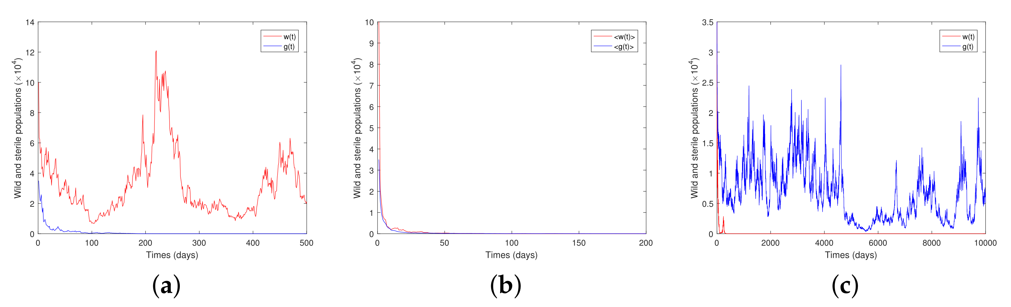
4. Persistence and Extinction

In this section, we will further explore the stochastic dynamic behavior of wild and sterile mosquito populations. We first give some definitions.

Definition 2

([45]). If ${lim}_{t\to \infty }w\left(t\right)=0,$ the species $w\left(t\right)$ is called extinction almost surely (a.s.)

Definition 3

([45]). If ${lim}_{t\to \infty }〈w\left(t\right)〉=0,$ population $w\left(t\right)$ is called stochastic non-persistence a.s. where $〈f\left(t\right)〉=t^{-1}{\int }_0^{t}f\left(s\right)ds.$

Definition 4

([45]). Population $w\left(t\right)$ is called stochastic permanence if for arbitrary $\epsilon >0,$ there are constants $\lambda >0,\chi >0$ such that

$${\mathbb{P}}_{\ast }=\left\{w\left(t\right)\ge \lambda \right\}\ge 1-\epsilon ,$$

and

$${\mathbb{P}}_{\ast }=\left\{w\left(t\right)\le \chi \right\}\ge 1-\epsilon .$$

4.1. Wild Mosquitoes

The threshold conditions of the extinction and persistence of wild mosquitoes are established in the following theorems.

Theorem 3.

If $a<{\mu }_1+{\sigma }_1^2/2$, then the population $w\left(t\right)$ will be extinct a.s.

Proof. 

For the first equation in System (2),

$$\mathrm{d}w=\left(\frac{aw}{w+g}-({\mu }_1+{\xi }_1(w+g))\right)w\mathrm{d}t+{\sigma }_{1}w\mathrm{d}{B}_1\left(t\right).$$

(9)

Applying Itô’s formula to Model (9) leads to

$$\mathrm{d}\ln w=\frac{1}{w}\mathrm{d}w-\frac{1}{2w^2}{\left(\mathrm{d}w\right)}^2=(\frac{aw}{w+g}-({\mu }_1+{\xi }_1(w+g))-\frac{{\sigma }_1^2}{2})\mathrm{d}t+{\sigma }_1\mathrm{d}{B}_1\left(t\right),$$

or, equivalently,

$$\ln (w\left(t\right)/w_0)={\int }_0^t[\frac{aw\left(s\right)}{w\left(s\right)+g\left(s\right)}-({\mu }_1+{\xi }_1(w\left(s\right)+g\left(s\right))-\frac{{\sigma }_1^2}{2})]\mathrm{d}s+{\sigma }_1{B}_1\left(t\right).$$

(10)

Therefore, we have

$$\ln (w\left(t\right)/w_0)\le (a-{\mu }_1-\frac{{\sigma }_1^2}{2})t-{\int }_0^t{\xi }_1(w\left(s\right)+g\left(s\right))\mathrm{d}s+{\sigma }_1{B}_1\left(t\right).$$

Similarly, we can show that

$$t^{-1}\ln (w\left(t\right)/w_0)+t^{-1}{\xi }_1{\int }_0^t(w\left(s\right)+g\left(s\right))\mathrm{d}s\le (a-{\mu }_1-\frac{{\sigma }_1^2}{2})+t^{-1}{\sigma }_1{B}_1\left(t\right).$$

Note that $a<{\mu }_1+\frac{{\sigma }_1^2}{2}$ and

$$\underset{t\to \infty }{lim}{B}_1\left(t\right)/t=0,$$

and for sufficiently large t, we have $a-{\mu }_1-\frac{{\sigma }_1^2}{2}\le \theta <0$ and ${\sigma }_1{B}_1\left(t\right)/t\le -\theta /2.$ Consequently,

$$t^{-1}\ln (w\left(t\right)/w_0)+t^{-1}{\xi }_1{\int }_0^t(w\left(s\right)+g\left(s\right))\mathrm{d}s\le \theta /2<0.$$

In addition, it follows from $w\left(t\right)\ge 0,g\left(t\right)\ge 0$ that $t^{-1}{\xi }_1{\int }_0^t(w\left(s\right)+g\left(s\right))ds\ge 0.$ Then, we get

$$t^{-1}\ln w\left(t\right)<0,$$

which is the required assertion. □

Inspired by [45], $\mathbb{P}\left(\overline{\mathsf{\Omega }}\right)=1,$ where

$$\overline{\mathsf{\Omega }}=\left\{\psi \in \mathsf{\Omega }:\underset{t\to \infty }{lim}w(\psi ,t)=0\right\},$$

for any $\psi \in \overline{\mathsf{\Omega }}$ and any small ${\delta }_1>0,$ there exists a constant $T_1(\psi ,{\delta }_1)>0$ such that

$$w(\psi ,t)<{\delta }_{1}fort\le T_1.$$

(11)

The following two theorems provide the threshold conditions of stochastic non-persistence and stochastic permanence for wild mosquitoes.

Theorem 4.

If $a={\mu }_1+{\sigma }_1^2/2,$ then the population $w\left(t\right)$ will be stochastically non-persistent a.s.

Proof. 

For arbitrarily fixed $\epsilon >0$, there exists a constant T such that

$${\sigma }_1{B}_1\left(t\right)<\epsilon t,$$

for $t>T$. Substituting this inequalities into Equation (10) gives

$$\begin{array}{cc}\hfill \ln (w\left(t\right)/w_0)& =-({\mu }_1+\frac{{\sigma }_1^2}{2})t+{\int }_0^t\frac{aw\left(s\right)}{w\left(s\right)+g\left(s\right)}\mathrm{d}s-{\xi }_1{\int }_0^t(w\left(s\right)+g\left(s\right))\mathrm{d}s+{\sigma }_1{B}_1\left(t\right)\hfill \\ \hfill & <(-{\mu }_1-\frac{{\sigma }_1^2}{2})t+at+{\sigma }_1{B}_1\left(t\right)-{\xi }_1{\int }_0^t(w\left(s\right)+g\left(s\right))\mathrm{d}s\hfill \\ \hfill & <(a-{\mu }_1-\frac{{\sigma }_1^2}{2})t+{\sigma }_1{B}_1\left(t\right)-{\xi }_1{\int }_0^{t}w\left(s\right)\mathrm{d}s\hfill \\ \hfill & <\epsilon t-{\xi }_1{\int }_0^{t}w\left(s\right)\mathrm{d}s,\hfill \end{array}$$

for all $t\ge T$ a.s. Let $u\left(t\right)={\int }_0^{t}w\left(s\right)\mathrm{d}s$. Then, we have

$$\ln (\mathrm{d}u/\mathrm{d}t)<\epsilon t-{\xi }_{1}u\left(t\right)+\ln w_0.$$

Taking the logarithm of both sides, for $t\ge T$, one has

$$\begin{array}{c}\hfill \exp \left({\xi }_{1}u\left(t\right)\right)\mathrm{d}h<w_0\exp \left(\epsilon t\right)\mathrm{d}t.\end{array}$$

Integrating this inequality from T to t yields

$$\exp \left({\xi }_{1}u\left(t\right)\right)<\frac{w_0{\xi }_1}{\epsilon }(\exp \left(\epsilon t\right)-\exp \left(\epsilon T\right))+\exp \left({\xi }_{1}u\left(T\right)\right).$$

That is,

$$u\left(t\right)<{\xi }_1^{-1}\ln [\frac{w_0{\xi }_1}{\epsilon }(\exp \left(\epsilon t\right)-\exp \left(\epsilon T\right)+\exp \left({\xi }_{1}u\left(T\right)\right)].$$

In other words, we have already shown that

$${\left\{{\int }_0^{t}w\left(s\right)\mathrm{d}s/t\right\}}^{\ast }<{\xi }_1^{-1}{\left\{\ln [\frac{w_0{\xi }_1}{\epsilon }(\exp \left(\epsilon t\right)-\exp \left(\epsilon T\right)+\exp \left({\xi }_{1}u\left(T\right)\right)]/t\right\}}^{\ast }.$$

An application of the L’Hospital’s rule results in

$${〈w\left(t\right)〉}^{\ast }\le \epsilon /{\xi }_1.$$

Since $\epsilon$ is arbitrary, we get ${〈w\left(t\right)〉}^{\ast }\le 0,$ proving the result. □

Theorem 5.

If $a>{\mu }_1+{\sigma }_1^2/2$ and $b<{\mu }_2+{\sigma }_2^2/2,$ then the population $w\left(t\right)$ will be stochastically permanent.

Proof. 

First, we show that for a given $\epsilon >0,$ there is a constant $\lambda >0$ such that ${\mathbb{P}}_{\ast }\left\{w\left(t\right)\ge \lambda \right\}\ge 1-\epsilon .$ Define $V_1\left(w\right)=1/w^2$ for $w\in R_{+}.$ Inspired by Liu [42] and applying Itô’s formula to Equation (9), we can see that

$$\begin{array}{cc}\hfill \mathrm{d}{V}_1\left(w\right)& =-2w^{-3}dw+3w^{-4}{\left(dw\right)}^2\hfill \\ \hfill & =-2w^{-2}[(\frac{aw}{w+g}-({\mu }_1+{\xi }_1(w+g))\mathrm{d}t+{\sigma }_{1}d{B}_1\left(t\right)]+3w^{-2}{\sigma }_1^2\mathrm{d}t\hfill \\ \hfill & =2V_1\left(w\right)[({\mu }_1+{\xi }_1(w+g)+1.5{\sigma }_1^2-\frac{aw}{w+g})\mathrm{d}t-{\sigma }_1\mathrm{d}{B}_1\left(t\right)].\hfill \end{array}$$

For any small $ϵ>0$ such that $a-{\mu }_1-0.5{\sigma }_1^2>ϵ>0,$ there is a positive constant $\theta$ satisfying

$$a-{\mu }_1-0.5{\sigma }_1^2-ϵ-\theta {\sigma }_1^2>0.$$

Define $V_2\left(w\right)={(1+V_1\left(w\right))}^{\theta }$ and by Equation (15), the application of Itô’s formula again leads to

$$\begin{array}{cc}\hfill \mathrm{d}{V}_2\left(w\right)=& \theta {(1+V_1\left(w\right))}^{\theta -1}d{V}_1+1/2\theta (\theta -1){(1+V_1\left(w\right))}^{\theta -2}{\left(\mathrm{d}{V}_1\right)}^2\hfill \\ \hfill =& \theta {(1+V_1\left(w\right))}^{\theta -2}[2V_1\left(w\right)(1+V_1\left(w\right))({\mu }_1+{\xi }_1(w+g)+1.5{\sigma }_1^2-\frac{aw}{w+g})+2\hfill \\ \hfill & \times (\theta -1)V_1{\left(w\right)}^2{\sigma }_1^2]dt-2\theta {(1+V_1\left(w\right))}^{\theta -1}{V}_1\left(w\right){\sigma }_1\mathrm{d}{B}_1\left(t\right)\hfill \\ \hfill \le & \theta {(1+V_1\left(w\right))}^{\theta -2}[-2(\frac{aw}{w+{\delta }_2}-{\mu }_1-{\xi }_1{\delta }_2-0.5{\sigma }_1^2-\theta {\sigma }_1^2)V_1^2\left(w\right)+2{\xi }_1{V}_1^{1.5}\left(w\right)\hfill \\ \hfill & +2({\mu }_1+{\xi }_1{\delta }_2+1.5{\sigma }_1^2-\frac{aw}{w+{\delta }_2})V_1\left(w\right)+2{\xi }_1{V}_1^{0.5}]\mathrm{d}t-2\theta {(1+V_1\left(w\right))}^{\theta -1}\hfill \\ \hfill & \times V_1\left(w\right){\sigma }_1\mathrm{d}{B}_1\left(t\right),\hfill \end{array}$$

for all $t\ge T_2.$ In view of $\mathbb{P}\left(\overline{\mathsf{\Omega }}\right)=1,$ we conclude

$$\begin{array}{cc}\hfill \mathrm{d}{V}_2\left(w\right)\le & \theta {(1+V_1\left(w\right))}^{\theta -2}[-2(a-{\mu }_1-0.5{\sigma }_1^2-\theta {\sigma }_1^2-ϵ)V_1^2\left(w\right)+2{\xi }_1{V}_1^{1.5}\left(w\right)\hfill \\ \hfill & +2({\mu }_1+1.5{\sigma }_1^2-a)V_1\left(w\right)+2{\xi }_1{V}_1^{0.5}]\mathrm{d}t-2\theta {(1+V_1\left(w\right))}^{\theta -1}{V}_1\left(w\right){\sigma }_1\mathrm{d}{B}_1\left(t\right),\hfill \end{array}$$

for $t\ge T_2.$ Now, we choose $\eta >0$ to be sufficiently small such that

$$\begin{array}{c}\hfill 0<\eta /\theta <2(a-{\mu }_1-0.5{\sigma }_1^2-\theta {\sigma }_1^2-ϵ).\end{array}$$

(12)

Define $V_3\left(w\right)=\exp \left(\eta t\right)V_2\left(w\right)=\exp \left(\eta t\right){(1+V_1\left(w\right))}^{\theta }.$ Making use of Itô’s formula yields

$$\begin{array}{cc}\hfill d{V}_3\left(w\left(t\right)\right)=& \eta \exp \left(\eta t\right)V_2\left(w\right)dt+\exp \left(\eta t\right)d{V}_2\left(w\right)\hfill \\ \hfill \le & \theta \exp \left(\eta t\right){(1+V_1\left(w\right))}^{\theta -2}[\eta /\theta {(1+V_1\left(w\right))}^2-2(a-{\mu }_1-0.5{\sigma }_1^2-\theta {\sigma }_1^2-ϵ)\hfill \\ \hfill & \times V_1{\left(w\right)}^2+2{\xi }_1{V}_1^{1.5}\left(w\right)+2({\mu }_1+1.5{\sigma }_1^2-a)V_1\left(w\right)+2{\xi }_1{V}_1^{0.5}\left(w\right)\left)\right]\mathrm{d}t\hfill \\ & -2\theta \exp \left(\eta t\right){(1+V_1\left(w\right))}^{\theta -1}{V}_1\left(w\right){\sigma }_1\mathrm{d}{B}_1\left(t\right)\hfill \\ \hfill =& \theta \exp \left(\eta t\right){(1+V_1\left(w\right))}^{\theta -2}[-2(a-{\mu }_1-0.5{\sigma }_1^2-\theta {\sigma }_1^2-ϵ-\eta /2\theta )V_1^2\left(w\right)\hfill \\ \hfill & +2{\xi }_1{V}_1^{1.5}+2({\mu }_1+1.5{\sigma }_1^2+\eta /\theta -a)V_1+2{\xi }_1{V}_1^{0.5}+\eta /\theta ]\mathrm{d}t\hfill \\ \hfill & -2\theta \exp \left(\eta t\right){(1+V_1\left(w\right))}^{\theta -1}{V}_1\left(w\right){\sigma }_1\mathrm{d}{B}_1\left(t\right),\hfill \\ \hfill :=& \exp \left(\eta t\right)F\left(w\right)\mathrm{d}t-2\theta \exp \left(\eta t\right){(1+V_1\left(w\right))}^{\theta -1}{V}_1\left(w\right){\sigma }_1\mathrm{d}{B}_1\left(t\right)\hfill \end{array}$$

for all $t\ge T_2.$ It follows from Equation (12) that $F\left(w\right)$ is upper bounded in $R_{+}$; namely, $F_1:={sup}_{x\in R_{+}}F\left(w\right)<+\infty .$ Thus,

$$d{V}_3\left(w\left(t\right)\right)\le F_1\exp \left(\eta t\right)dt-2\theta \exp \left(\eta t\right){(1+V_1\left(w\right))}^{\theta -1}{V}_1\left(w\right){\sigma }_{1}d{B}_1\left(t\right).$$

Integrating both sides and then taking expectations gives

$$E\left[\exp \left(\eta t\right){(1+V_1\left(w\left(t\right)\right))}^{\theta }\right]\le {(1+V_1\left(w_0\right))}^{\theta }+F_1(\exp \left(\eta t\right)-1)/\eta .$$

The superior limit results in

$$\underset{t\to \infty }{lim\; sup}E\left[w^{-2\theta \left(t\right)}\right]=\underset{t\to \infty }{lim\; sup}E\left[V_1^{\theta }\left(w\left(t\right)\right)\right]\le \underset{t\to \infty }{lim\; sup}E\left[{(1+V_1\left(w\left(t\right)\right))}^{\theta }\right]\le F_1/\eta :=F_2.$$

Thus, for any given $\epsilon >0,$ let $\lambda ={\epsilon }^{0.5/\theta }/F_2^{0.5/\theta },$ Chebyshev’s inequality leads to

$$\mathbb{P}\left\{w\left(t\right)<\lambda \right\}=\left\{w^{-2\theta }\left(t\right)>{\lambda }^{-2\theta }\right\}\le E\left[w^{-2\theta }\left(t\right)\right]/{\lambda }^{-2\theta }={\lambda }^{2\theta }E\left[w^{-2\theta }\left(t\right)\right],$$

i.e., ${\mathbb{P}}^{\ast }\left\{w\left(t\right)<\lambda \right\}\le {\lambda }^{2\theta }{F}_2=\epsilon .$ Therefore,

$${\mathbb{P}}_{\ast }\left\{w\left(t\right)\ge \lambda \right\}\ge 1-\epsilon .$$

Next, we prove that for arbitrary fixed $\epsilon >0,$ there exists $\chi >0$ such that

$${\mathbb{P}}_{\ast }\left\{w\left(t\right)\le \chi \right\}\ge 1-\epsilon .$$

To this end, we define $V\left(w\right)=w^q$ for $w\in R_{+}$, where $0<q<1.$ Then, it follows from Itô’s formula that

$$\begin{array}{cc}\hfill \mathrm{d}V\left(w\right)& =q{w}^{w-1}\mathrm{d}w+\frac{q(q-1)}{2}{w}^{q-2}{\left(\mathrm{d}w\right)}^2\hfill \\ \hfill & =q{w}^q\left\{[\frac{aw}{w+g}-({\mu }_1+\xi (w+g))+(q-1){\sigma }_1^2/2]\mathrm{d}t+{\sigma }_1\mathrm{d}{B}_1\left(t\right)\right\}.\hfill \end{array}$$

Let $k_0>0$ be large enough such that $w_0\in [1/k_0,k_0].$ For each integer $k\ge k_0,$ define the stopping time ${\tau }_k=inf\left\{t\ge 0:w\left(t\right)\notin (1/k,k)\right\}.$ Clearly, ${\tau }_k\to \infty$ when $k\to \infty$ a.s. Applying Itô’s formula again to $\exp \left(t\right)V\left(w\right)$ gives

$$\begin{array}{cc}\hfill \mathrm{d}\left(\exp \right(t\left)V\right(w\left)\right)=& \exp \left(t\right)V\left(w\right)\mathrm{d}t+\exp \left(t\right)\mathrm{d}V\left(w\right)\hfill \\ \hfill =& \exp \left(t\right)\left\{w^q+q{w}^q[\frac{aw}{w+g}-({\mu }_1+{\xi }_1(w+g))-\frac{(1-q){\sigma }_1^2}{2}]\mathrm{d}t\right\}\hfill \\ \hfill & +\exp \left(t\right)q{w}^q{\sigma }_1\mathrm{d}{B}_1\left(t\right)\hfill \\ \hfill \le & \exp \left(t\right)[w^q+q{w}^q(a-{\mu }_1-\frac{(1-q){\sigma }_1^2}{2}-{\xi }_{1}w)]\mathrm{d}t+\exp \left(t\right)q{w}^q{\sigma }_1\mathrm{d}{B}_1\left(t\right)\hfill \\ \hfill \le & \exp \left(t\right)M+\exp \left(t\right)q{w}^q{\sigma }_1\mathrm{d}{B}_1\left(t\right),\hfill \end{array}$$

where M is a positive constant. Integrating this inequality and taking expectations on both sides, one can see that

$$E\left[\exp \left(t^{{\tau }_k}\right)w^q\left(t^{{\tau }_k}\right)\right]-w_0^q\le M(\exp \left(t\right)-1).$$

Letting $k\to \infty$ yields

$$E\left[w^q\left(t\right)\right]\le \exp (-t)w_q^0+M.$$

In other words, we have already shown that ${\displaystyle \underset{t\to +\infty }{lim\; sup}}E\left[w^q\left(t\right)\right]\le M.$ Thus, for any given $\epsilon >0,$ let $\chi =K^{1/q}/{\epsilon }^{1/q},$ by virtue of Chebyshev’s inequality, we can derive that

$$\mathbb{P}\left\{w\left(t\right)>\chi \right\}=\mathbb{P}\left\{w^q\left(t\right)>{\chi }^q\right\}\le E\left[w^q\left(t\right)\right]/{\chi }^q;$$

that is to say, ${\mathbb{P}}^{\ast }\left\{w\left(t\right)>\chi \right\}\le \epsilon .$ Consequently, ${\mathbb{P}}_{\ast }\left\{w\left(t\right)\le \chi \right\}\ge 1-\epsilon .$ □

4.2. Sterile Mosquitoes

We establish the threshold conditions of the extinction and persistence of sterile mosquitoes in the following three theorems.

Theorem 6.

If $b<{\mu }_2+{\sigma }_2^2/2,$ then the population $g\left(t\right)$ will be extinct a.s.

Proof. 

For the second equation in System (2),

$$\mathrm{d}g=\left(b-({\mu }_2+{\xi }_2(w+g))\right)g\mathrm{d}t+{\sigma }_{2}g\mathrm{d}{B}_2\left(t\right).$$

(13)

Applying Itô’s formula to Equation (13) leads to

$$\mathrm{d}\ln g=\frac{1}{g}\mathrm{d}g-\frac{{\left(\mathrm{d}g\right)}^2}{2g^2}=(b-({\mu }_2+{\xi }_2(w+g))-\frac{{\sigma }_2^2}{2})\mathrm{d}t+{\sigma }_2\mathrm{d}{B}_2\left(t\right).$$

Integrating both sides of the above inequality from 0 to t, we get

$$\ln g\left(t\right)-\ln g_0=(b-{\mu }_2-\frac{{\sigma }_{2^2}}{2})t-{\xi }_2{\int }_0^t(w\left(s\right)+g\left(s\right))\mathrm{d}s+{\sigma }_2{B}_2\left(t\right).$$

(14)

That is,

$$t^{-1}\ln (g\left(t\right)/g_0)+t^{-1}{\xi }_2{\int }_0^t(w\left(s\right)+g\left(s\right))\mathrm{d}s=(b-{\mu }_2-\frac{{\sigma }_2^2}{2})+t^{-1}{\sigma }_2{B}_2\left(t\right).$$

Let $b<{\mu }_2+\frac{{\sigma }_2^2}{2}$ and

$$\underset{t\to \infty }{lim}=\frac{B_2\left(t\right)}{t}=0.$$

For any $\theta ,$ we have $b-{\mu }_2-\frac{{\sigma }_2^2}{2}\le \theta <0$ and ${\sigma }_2{B}_2\left(t\right)/t\le -\frac{\theta }{2}$; then,

$$t^{-1}\ln (g\left(t\right)/g_0)+t^{-1}{\xi }_2{\int }_0^t(w\left(s\right)+g\left(s\right))\mathrm{d}s\le \theta /2<0.$$

It is obvious that $w\left(t\right)\ge 0$ and $g\left(t\right)\ge 0.$ Therefore, we get

$$t^{-1}\ln g\left(t\right)<0,$$

which implies that sterile mosquitoes will be extinct. □

It follows from Theorem 6 that $\mathbb{P}\left(\overline{\mathsf{\Omega }}\right)=1$, where

$$\overline{\mathsf{\Omega }}=\left\{\psi \in \mathsf{\Omega }:\underset{t\to \infty }{lim}g(\psi ,t)=0\right\}.$$

Then, for any $\psi \in \overline{\mathsf{\Omega }}$ and any small ${\delta }_2>0,$ there exists a constant $T_2(\psi ,{\delta }_2)>0$ such that

$$g(\psi ,t)<{\delta }_{2}fort\ge T_2.$$

(15)

Theorem 7.

If $b={\mu }_2+{\sigma }_2^2/2,$ then the population $g\left(t\right)$ will be stochastically non-persistent.

Proof. 

For any $\eta >0,$ there exists a constant T such that

$${\sigma }_2{B}_2\left(t\right)<\eta t,$$

for $t>T$. Together with Equation (14), we have

$$\begin{array}{cc}\hfill \ln (g\left(t\right)/g_0)& =(b-{\mu }_2-\frac{{\sigma }_2^2}{2})t-{\xi }_2{\int }_0^t(w\left(s\right)+g\left(s\right))\mathrm{d}s+{\sigma }_2{B}_2\left(t\right)\hfill \\ \hfill & <(b-{\mu }_2-\frac{{\sigma }_2^2}{2})t-{\xi }_2{\int }_0^{t}g\left(s\right)\mathrm{d}s+{\sigma }_2{B}_2\left(t\right)\hfill \\ \hfill & <\eta t-{\xi }_2{\int }_0^{t}g\left(s\right)\mathrm{d}s.\hfill \end{array}$$

Let $f\left(t\right)={\int }_0^{t}g\left(s\right)\mathrm{d}s$. The above inequality can be rewritten as

$$\ln (\mathrm{d}f/\mathrm{d}t)<\eta t-{\xi }_{2}f\left(t\right)+\ln g_0.$$

Then,

$$f\left(t\right)<{\xi }_2^{-1}\ln [g_0{\xi }_2/\eta (\exp \left\{\eta t\right\}-\exp \left\{\eta T\right\})+\exp \left\{{\xi }_{2}f\left(T\right)\right\}].$$

After taking the upper bound and L’Hospital’s of the above inequality,

$${〈g\left(t\right)〉}^{\ast }\le \eta /{\xi }_2,$$

proving the result. □

Theorem 8.

If $b>{\mu }_2+{\sigma }_2^2/2$ and $a<{\mu }_1+{\sigma }_1^2/2,$ then the population $g\left(t\right)$ will be stochastically permanent a.s.

Proof. 

We first demonstrate that for any $\epsilon >0,$ there exists a constant ${\lambda }^{{}^{\prime }}>0$ such that ${\mathbb{P}}_{\ast }\left\{g\left(t\right)\ge {\lambda }^{{}^{\prime }}\right\}\ge 1-\epsilon .$ Define $V_1\left(g\right)=1/g^2$ for $g\in R_{+}.$ Applying Itô’s formula to Equation (13), we obtain

$$\begin{array}{cc}\hfill \mathrm{d}{V}_1& =-2g^{-3}\mathrm{d}g+3g^{-4}{\left(\mathrm{d}g\right)}^2\hfill \\ \hfill & =[-2g^{-2}(b-{\mu }_2-{\xi }_2(w+g))+3g^{-2}{\sigma }_2^2]\mathrm{d}t-2g^{-2}{\sigma }_2\mathrm{d}{B}_2\left(t\right)\hfill \\ \hfill & =2V_1[{\mu }_2+{\xi }_2(w+g)-b+1.5{\sigma }_2^2]\mathrm{d}t-2V_1{\sigma }_2\mathrm{d}{B}_2\left(t\right).\hfill \end{array}$$

For any $ϵ$ satisfying $b-{\mu }_2-0.5{\sigma }_2^2>ϵ>0,$ we can choose a positive constant $\theta$ such that

$$b-{\mu }_2-0.5{\sigma }_2^2-\theta {\sigma }_2^2-ϵ>0.$$

Next, define $V_2={(1+V_1\left(g\right))}^{\theta }$. Then, from Equation (11), we get

$$\begin{array}{cc}\hfill \mathrm{d}{V}_2\left(g\right)=& \theta {(1+V_1\left(g\right))}^{\theta -1}\mathrm{d}{V}_1+\frac{1}{2}\theta (\theta -1){(1+V_1\left(g\right))}^{\theta -2}{\left(\mathrm{d}{V}_1\right)}^2\hfill \\ \hfill =& \theta {(1+V_1\left(g\right))}^{\theta -2}[2V_1(1+V_1)({\mu }_2+{\xi }_2(w+g)+1.5{\sigma }_2^2-b)+2(\theta -1){\sigma }_2^2\hfill \\ \hfill & \times V_1^2\left(g\right)]\mathrm{d}t-2\theta {(1+V_1)}^{\theta -1}{V}_1\left(g\right){\sigma }_2\mathrm{d}{B}_2\left(t\right)\hfill \\ \hfill =& \theta {(1+V_1\left(g\right))}^{\theta -2}[2({\mu }_2+0.5{\sigma }_2^2+\theta {\sigma }_2^2+{\xi }_2{\delta }_1-b)V_1^2\left(g\right)+2{\xi }_2{V}_1^{1.5}\left(g\right)+2({\mu }_2\hfill \\ \hfill & +1.5{\sigma }_2^2+{\xi }_2{\delta }_1-b)V_1\left(g\right)+2{\xi }_2{V}_1^{0.5}\left(g\right)]\mathrm{d}t-2\theta {(1+V_1\left(g\right))}^{\theta -1}{V}_1\left(g\right){\sigma }_2\mathrm{d}{B}_2\left(t\right),\hfill \end{array}$$

for $t\ge T_1.$ With $\mathbb{P}\left(\overline{\mathsf{\Omega }}\right)=1$, one has

$$\begin{array}{cc}\hfill \mathrm{d}{V}_2\left(g\right)\le & \theta {(1+V_1\left(g\right))}^{\theta -2}[-2(b-{\mu }_2-0.5{\sigma }_2^2-\theta {\sigma }_2^2-ϵ)V_1^2\left(g\right)+2{\xi }_2{V}_1^{1.5}\left(g\right)+2({\mu }_2\hfill \\ \hfill & +b+1.5{\sigma }_2^2)V_1\left(g\right)+2{\xi }_2{V}_1^{0.5}\left(g\right)]\mathrm{d}t-2\theta {(1+V_1\left(g\right))}^{\theta -1}{V}_1\left(g\right){\sigma }_2\mathrm{d}{B}_2\left(t\right).\hfill \end{array}$$

Now, let $\eta >0$ be sufficiently small such that

$$0<\eta /\theta <2(b-{\mu }_2-0.5{\sigma }_2^2-\theta {\sigma }_2^2-ϵ).$$

Define $V_3=\exp \left(\eta t\right)V_2\left(g\right).$ By virtue of Itô’s formula,

$$\begin{array}{cc}\hfill \mathrm{d}{V}_3\left(g\left(t\right)\right)=& \eta \exp \left(\eta t\right)V_2\left(g\right)\mathrm{d}t+\exp \left(\eta t\right)\mathrm{d}{V}_2\left(g\right)\hfill \\ \hfill \le & \exp \left(\eta t\right)\theta {(1+V_1\left(g\right))}^{\theta -2}[\eta /\theta {(1+V_1\left(g\right))}^2-2(b-{\mu }_2-0.5{\sigma }_2^2-\theta {\sigma }_2^2-ϵ)V_1^2\left(g\right)\hfill \\ \hfill & +2{\xi }_2{V}_1^{1.5}\left(g\right)+2({\mu }_2+b+1.5{\sigma }_2^2)V_1\left(g\right)+2{\xi }_2{V}_1^{0.5}]\mathrm{d}t-2\theta {(1+V_1\left(g\right))}^{\theta -1}{V}_1\left(g\right)\hfill \\ \hfill & \times {\sigma }_2\mathrm{d}{B}_2\left(t\right)\hfill \\ \hfill \le & \exp \left(\eta t\right)\theta {(1+V_1\left(g\right))}^{\theta -2}[-2(b-{\mu }_2-0.5{\sigma }_2^2-\theta {\sigma }_2^2-ϵ-0.5\eta /\theta )V_1^2\left(g\right)\hfill \\ \hfill & +2{\xi }_2{V}_1^{1.5}\left(g\right)+2({\mu }_2+b+1.5{\sigma }_2^2+\eta /\theta )V_1\left(g\right)+2{\xi }_2{V}_1^{0.5}\left(g\right)+\eta /\theta ]\mathrm{d}t\hfill \\ \hfill & -2\exp \left(\eta t\right)\theta {(1+V_1\left(g\right))}^{\theta -1}{V}_1\left(g\right){\sigma }_2\mathrm{d}{B}_2\left(t\right)\hfill \\ \hfill =& :\exp \left(\eta t\right)H\left(g\right)\mathrm{d}t-2\exp \left(\eta t\right)\theta {(1+V_1\left(g\right))}^{\theta -1}{V}_1\left(g\right){\sigma }_2\mathrm{d}{B}_2\left(t\right),\hfill \end{array}$$

for $t\ge T_1.$ Note that $H\left(g\right)$ is upper bounded in $R_{+}$, i.e.,

$$H_1:\underset{g\in R_{+}}{sup}H\left(g\right)<\infty .$$

Consequently,

$$\mathrm{d}{V}_3\left(g\left(t\right)\right)\le H_1\exp \left(\eta t\right)\mathrm{d}t-2\exp \left(\eta t\right)\theta {(1+V_1\left(g\right))}^{\theta -1}{V}_1\left(g\right){\sigma }_2\mathrm{d}{B}_2\left(t\right),$$

for $t\ge T_1.$ Integrating both sides of the above inequality and taking expectations give

$$E\left[\exp \left(\eta t\right){(1+V_1\left(g\left(t\right)\right))}^{\theta }\right]\le {(1+V_1\left(g_0\right))}^{\theta }+H_1(\exp \left(\eta t\right)-1)/\eta .$$

In other words, we have

$$\underset{t\to \infty }{lim\; sup}E\left[V_1^{\theta }\left(g\left(t\right)\right)\right]\le \underset{t\to \infty }{lim\; sup}E[(1+V_1{\left(g\left(t\right)\right)}^{\theta }]\le H_1/\eta .$$

That is to say,

$$\underset{t\to \infty }{lim\; sup}E\left[g^{-2\theta }\left(t\right)\right]\le H_1/\eta =:H_2.$$

Thus, for any given $\epsilon >0,$ and when ${\lambda }_1^{{}^{\prime }}={\epsilon }^{1/2\theta }/H_2^{1/2\theta },$ by Chebyshev’s inequality,

$$\mathbb{P}\left\{g\left(t\right)<{\lambda }^{{}^{\prime }}\right\}=\mathbb{P}\left\{g^{-2\theta }\left(t\right)>{\left({\lambda }^{{}^{\prime }}\right)}^{-2\theta }\right\}\le E\left[g^{-2\theta }\left(t\right)\right]/{\left({\lambda }^{{}^{\prime }}\right)}^{-2\theta }={\left({\lambda }^{{}^{\prime }}\right)}^{2\theta }E\left[g^{-2\theta }\left(t\right)\right].$$

That is to say, ${\mathbb{P}}^{\ast }\left\{g\left(t\right)<{\lambda }^{{}^{\prime }}\right\}\le \epsilon .$

Thus, ${\mathbb{P}}_{\ast }\left\{g\left(t\right)\ge {\lambda }^{{}^{\prime }}\right\}\ge 1-\epsilon .$

Next, we prove that for arbitrary fixed $\epsilon >0,$ there exists ${\chi }^{{}^{\prime }}>0$ such that

$${\mathbb{P}}_{\ast }\left\{g\left(t\right)\le {\chi }^{{}^{\prime }}\right\}\ge 1-\epsilon .$$

To this end, we define $V\left(g\right)=g^p$ for $g\in R_{+},$ where $0<p<1.$ Then,

$$\begin{array}{c}\hfill \mathrm{d}V\left(g\right)=p{g}^p(b-{\mu }_2-{\xi }_2(w+g)+\frac{(p-1)}{2}{\sigma }_2^2)\mathrm{d}t+p{g}^p{\sigma }_2\mathrm{d}{B}_2\left(t\right).\end{array}$$

Let $k_0>0$ be large enough such that $g_0\in [1/k_0,k_0].$ For each integer $k\ge k_0,$ define the stopping time ${\tau }_k=\left\{inf:g\left(t\right)\notin (1/k,k)\right\}.$ Clearly, ${\tau }_k\to \infty$ almost surely as $k\to \infty .$ Applying Itô’s formula again to $\exp \left(t\right)V\left(g\right)$ gives

$$\begin{array}{cc}\hfill \mathrm{d}\left(\exp \right(t\left)V\right(g\left)\right)=& \exp \left(t\right)\left\{g^p+p{g}^p[b-{\mu }_2-{\xi }_2(w+g)+0.5(p-1){\sigma }_2^2]\right\}\mathrm{d}t\hfill \\ \hfill & +\exp \left(t\right)p{g}^p{\sigma }_2\mathrm{d}{B}_2\left(t\right)\hfill \\ \hfill \le & \exp \left(t\right)g^p[1+p(b-{\mu }_2-{\xi }_{2}g+0.5(p-1){\sigma }_2^2)]\mathrm{d}t+\exp \left(t\right)p{g}^p{\sigma }_2\mathrm{d}{B}_2\left(t\right)\hfill \\ \hfill \le & \exp \left(t\right)M+\exp \left(t\right)p{g}^p{\sigma }_2\mathrm{d}{B}_2\left(t\right),\hfill \end{array}$$

where M is a positive constant. Furthermore, we get

$$\underset{t\to \infty }{lim\; sup}E\left[g^p\left(t\right)\right]\le M.$$

Thus, for any given $\epsilon >0,$ let ${\chi }^{{}^{\prime }}=M^{1/p}/{\epsilon }^{1/p},$ by virtue of Chebyshev’s inequality, we can derive that

$${\mathbb{P}}^{\ast }\left\{g\left(t\right)>{\chi }^{{}^{\prime }}\right\}\le \epsilon .$$

Namely,

$${\mathbb{P}}_{\ast }\left\{g\left(t\right)\le {\chi }^{{}^{\prime }}\right\}\ge 1-\epsilon .$$

End of certification. □

5. Discussion

Releasing sterile mosquitoes to suppress or even eradicate wild female mosquitoes has been proven to be an effective method to combat mosquito-borne diseases (MBDs) [10,11,13,18,19,20,21,22,23,24], and various determinative models have been developed to study the interactive dynamics of wild and sterile mosquitoes [11,18,19,25,26,27,28,29,30,31,32,33,34,35,36]. However, all these models did not consider the effect of random environmental changes on the dynamics of mosquito populations. To fill this gap, in the current paper we develop a random interactive wild and sterile mosquito population model embedded with white noise to characterize the effect of a random environment on the death rates of mosquitoes. By constructing suitable Lyapunov functions and applying the Itô’s formula, we discuss the existence and uniqueness of the global positive solution and stochastically ultimate boundedness of solutions for System (2), as well as the extinction and persistence of wild and sterile mosquitoes. Our theoretical results on the threshold conditions for the extinction, non-persistence, and stochastic permanence of wild mosquito $w\left(t\right)$ and sterile mosquito $g\left(t\right)$ are listed as follows.

(i)

If $a<{\mu }_1+{\sigma }_1^2/2,$ then $w\left(t\right)$ will go to extinction.

(ii)

If $a={\mu }_1+{\sigma }_1^2/2,$ then $w\left(t\right)$ will be stochastically non-persistent.

(iii)

If $a>{\mu }_1+{\sigma }_1^2/2$ and $b<{\mu }_2+{\sigma }_2^2/2,$ then $w\left(t\right)$ will be stochastically permanent.

(iv)

If $b<{\mu }_2+{\sigma }_2^2/2,$ then $g\left(t\right)$ will go to extinction.

(v)

If $b={\mu }_2+{\sigma }_2^2/2,$ then $g\left(t\right)$ will be stochastically non-persistent.

(vi)

If $b>{\mu }_2+{\sigma }_2^2/2$ and $a<{\mu }_1+{\sigma }_1^2/2,$ then $g\left(t\right)$ will be stochastically permanent.

The above results show that different combinations of the white noise ${\sigma }_i$ with $i=1,2$ may results different fates for wild and sterile mosquitoes. To see this numerically, we fix other parameters and vary ${\sigma }_1$ and ${\sigma }_2$ to explore the influence of white noise on the dynamic behaviors of sterile and wild mosquitoes. Before numerical simulation, we use the Milstein’s higher order method for showing approximate solutions with initial conditions [46]. We can rewrite $(w,g)$ as $(x,y)$ for convenience and obtain discretization equations of Model (2) as follows

$$\left\{\begin{array}{c}{x}_{k+1}=x_k+(a{x}_k/(x_k+y_k)-({\mu }_1+{\xi }_1(x_k+y_k)))x_k\mathrm{\Delta }t+{\sigma }_1{x}_k\sqrt{\mathrm{\Delta }t}+0.5{\sigma }_1^2{x}_k({\alpha }_k^2-1)\mathrm{\Delta }t,\hfill \\ \\ y_{k+1}=y_k+(b-({\mu }_2+{\xi }_2(x_k+y_k)))y_k\mathrm{\Delta }t+{\sigma }_2{y}_k\sqrt{\mathrm{\Delta }t}+0.5{\sigma }_2^2{y}_k({\beta }_k^2-1)\mathrm{\Delta }t,\hfill \end{array}\right.$$

where the step size $\mathrm{\Delta }t=0.01.$ Making use of the numerical simulation method given above, we give the following figures by fix ${\sigma }_i.$ In Figure 1, we set ${\mu }_1={\xi }_1=0.5,$ ${\mu }_2={\xi }_2=0.4,$ $a=2,$ $b=0.5,$ $w_0=10$ and vary ${\sigma }_i$. In Figure 1a, we let ${\sigma }_1=2$ and ${\sigma }_2=1$ such that the condition of Theorem 3 is satisfied ($a<2.5={\mu }_1+{\sigma }_1^2/2$), and the population w will go to extinction. In Figure 1b, where $〈w\left(t\right)〉=t^{-1}{\int }_0^{s}w\left(s\right)ds$ and $〈g\left(t\right)〉=t^{-1}{\int }_0^{s}g\left(s\right)ds$, we choose ${\sigma }_1=3^{1/2}$ and ${\sigma }_2=1$ such that the condition in Theorem 4 ($a=2={\mu }_1+{\sigma }_1^2/2$) is satisfied. In such a case, the population w will be stochastically non-persistent. In Figure 1c, we choose ${\sigma }_1=0.76,{\sigma }_2=2$ such that ($a>0.7888={\mu }_1+{\sigma }_1^2/2$), and hence Theorem 5 guarantees that the population w will be stochastically permanent.

Regarding the dynamics of population g, in Figure 2 we set ${\mu }_1={\xi }_1=0.5,{\mu }_2={\xi }_2=0.4,a=2,b=0.9,g_0=3.5$ and made ${\sigma }_i$ a variable. Figure 2a is for ${\sigma }_1=1.2$ and ${\sigma }_2=2$, which makes $b<2.4={\mu }_2+{\sigma }_2^2/2$ satisfied in Theorem 6, and therefore, population g will go to extinction. In Figure 2b, we choose ${\sigma }_1=2,{\sigma }_2=1$, and hence the condition $b=0.9={\mu }_2+{\sigma }_2^2/2$ in Theorem 7 is met and population g will be stochastically non-persistent, while selecting ${\sigma }_1=2$ and ${\sigma }_2=0.6$ such that the condition $b>0.58={\mu }_2+{\sigma }_2^2/2$ of Theorem 8 is satisfied, Figure 2c shows that population g will be stochastically permanent. Furthermore, when exploring the stochastic permanence of g, it is found that properly increasing the value of the b can make the dynamic behavior of g population clearer. This also confirms some of the conclusions of [47] . It means that many complicating factors can be dealt with simply by b.

To sum up, both theoretical results and numerical simulations show that different combinations of white noise result in different dynamics of wild and sterile mosquitoes. The white noise brought by a random environment affects the mosquito control strategy. Figure 1 shows that wild females will go from extinction, through stochastic non-persistence, to stochastic permanence as the noise intensity ${\sigma }_1$ decreases. Figure 2 manifests a similar fate for sterile mosquitoes in that they go through extinction, are stochastically non-persistent and stochastically persistent as the noise intensity ${\sigma }_2$ decreases. It is well-recognized that the survival of mosquitoes is highly related to their living conditions, which are random; hence, it is a meaningful topic to discuss the effect of different types of noise on the persistence and extinction of the mosquito populations. We made our first attempt in this paper, and our future work will include different release strategies in model development.

References

1. Caraballo, H.; King, K. Emergency department management of mosquito-borne illness: Malaria, dengue, and west nile virus. Emerg. Med. Pract. 2014, 16, 1–23. [Google Scholar] [PubMed]
2. Bian, G.; Joshi, D.; Dong, Y.; Lu, P.; Zhou, G.; Pan, X.; Xu, Y.; Dimopoulos, G.; Xi, Z. Wolbachia invades anopheles stephensi populations and induces refractoriness to plasmodium infection. Science 2013, 340, 748–751. [Google Scholar] [CrossRef] [PubMed]
3. Dutra, H.; Rocha, M.; Dias, F.; Mansur, S.B.; Caragata, E.P.; Moreira, L.A. Wolbachia blocks currently circulating Zika virus isolates in brazilian Aedes aegypti mosquitoes. Cell Host Microbe 2016, 19, 771–774. [Google Scholar] [CrossRef] [PubMed] [Green Version]
4. Epstein, P.R.; Diaz, H.F.; Elias, S.; Grabherr, G.; Graham, N.E.; Martens, W.J.; MosIey-Thompson, E.; Susskind, J. Biological and physical signs of climate change: Focus on mosquito-borne diseases. Bull. Am. Meteorol. Soc. 1988, 79, 409–417. [Google Scholar] [CrossRef] [Green Version]
5. Tolle, M.A. Mosquito-borne diseases. Curr. Probl. Pediatr. Adolesc. Health Care 2009, 39, 97–140. [Google Scholar] [CrossRef]
6. Chye, J.K.; Lim, C.T.; Ng, K.B.; Lim, J.M.; George, R.; Lam, S.K. Vertical transmission of dengue. Clin. Infect. Dis. 1997, 25, 1374–1377. [Google Scholar] [CrossRef] [Green Version]
7. Berg, H.V.D. Global status of DDT and its alternatives for use in vector control to prevent disease. Ciência Saúde Coletiva 2009, 117, 1656–1663. [Google Scholar]
8. Lambrechts, L.; Ferguson, N.M.; Harris, E.; Holmes, E.C.; McGraw, E.A.; O’Neill, S.L.; Ooi, E.E.; Ritchie, S.A.; Ryan, P.A.; Scott, T.W.; et al. Assessing the epidemiological effect of Wolbachia for dengue control. Lancet Infect. Dis. 2017, 15, 862–866. [Google Scholar] [CrossRef] [Green Version]
9. Okumu, F.O.; Moore, S.J. Combining indoor residual spraying and insecticide-treated nets for malaria control in Africa: A review of possible outcomes and an outline of suggestions for the future. Malar. J. 2011, 10, 208. [Google Scholar] [CrossRef] [Green Version]
10. Li, J. Differential equations models for interacting wild and transgenic mosquito populations. J. Biol. Dyn. 2008, 241–258. [Google Scholar] [CrossRef] [Green Version]
11. Barclay, H.J.; Mackuer, M. The sterile insect release method for pest control: A density dependent model. Environ. Entomol. 1980, 9, 810–817. [Google Scholar] [CrossRef]
12. Dumont, Y.; Tchuenche, J.M. Mathematical studies on the sterile insect technique for the Chikungunya disease and Aedes albopictus. J. Math. Biol. 2012, 65, 809–854. [Google Scholar] [CrossRef]
13. Dyck, V.; Hendrichs, J.P.; Robinson, A.S. Sterile insect technique principles and practice in area-wide integrated pest management. New Agric. 2005, 1, 147–174. [Google Scholar]
14. Esteva, L.; Yang, H.M. Mathematical model to assess the control of Aedes aegypti mosquitoes by the sterile insect technique. Math. Biosci. 2005, 198, 132–147. [Google Scholar] [CrossRef]
15. Ito, J.; Ghosh, A.; Moreira, L.A.; Wilmmer, E.A.; Jacobs-Lorena, M. Transgenic anopheline mosquitoes impaired in transmission of a malria parasite. Nature 2002, 417, 452–455. [Google Scholar] [CrossRef]
16. Rafikov, M.; Bevilacqua, L.; Wyse, A. Optimal control strategy of malaria vector using genetically modified mosquitoes. J. Theor. Biol. 2009, 258, 418–425. [Google Scholar] [CrossRef]
17. Thome, R.C.A.; Yang, H.M.; Esteva, L. Optimal control of Aedes aegypti mosquitoes by the sterile insect technique and insecticide. Math. Biosci. 2010, 223, 12–23. [Google Scholar] [CrossRef]
18. Yu, J.; Zheng, B. Modeling Wolbachia infection in mosquito population via discrete dynamical models. J. Differ. Equ. 2019, 25, 1549–1567. [Google Scholar] [CrossRef]
19. Cai, L.; Ai, S.; Li, J. Dynamics of mosquitoes populations with different strategies for releasing sterile mosquitoes. SIAM J. Appl. Math. 2014, 74, 1786–1809. [Google Scholar] [CrossRef]
20. Hoffmann, A.A.; Montgomery, B.L.; Popovici, J.; Iturbe-Ormaetxe, I.; Johnson, P.H.; Muzzi, F.; Greenfield, M.; Durkan, M.; Leong, Y.S.; Dong, Y.; et al. Successful establishment of Wolbachia in Aedes populations to suppress dengue transmission. Nature 2011, 476, 454–457. [Google Scholar] [CrossRef]
21. Reiter, P. Oviposition, dispersal, and survival in Aedes aegypti: Implications for the efficacy of control strategies. Vector-Borne Zoonotic Dis. 2007, 7, 261–273. [Google Scholar] [CrossRef]
22. Walker, T.; Johnson, P.H.; Moreira, L.A.; Iturbe-Ormaetxe, I.; Frentiu, F.D.; McMeniman, C.J.; Leong, Y.S.; Dong, Y.; Axford, J.; Kriesner, P.; et al. The wMel Wolbachia strain blocks dengue and invades caged Aedes aegypti populations. Nature 2011, 476, 450–453. [Google Scholar] [CrossRef]
23. Yu, J.; Li, J. Global asymptotic stability in an interactive wild and sterile mosquito model. J. Differ. Equ. 2020, 7, 6193–6215. [Google Scholar] [CrossRef]
24. Zheng, X.; Zhang, D.; Li, Y.; Yang, C.; Wu, Y.; Liang, X.; Liang, Y.; Pan, X.; Hu, L.; Sun, Q.; et al. Incompatible and sterile insect techniques combined eliminate mosquitoes. Nature 2019, 572, 56–61. [Google Scholar] [CrossRef]
25. Li, J.; Cai, L.; Li, Y. Stage-structured wild and sterile mosquito population models and their dynamics. J. Biol. Dyn. 2016, 11, 79–101. [Google Scholar] [CrossRef]
26. Li, J. New revised simple models for interactive wild and sterile mosquito populations and their dynamics. J. Biol. Dyn. 2017, 11, 316–333. [Google Scholar] [CrossRef] [Green Version]
27. Huang, M.; Song, X.; Li, J. Modeling and analysis of impulsive releases of sterile mosquitoes. J. Biol. Dyn. 2017, 11, 147–171. [Google Scholar] [CrossRef] [Green Version]
28. Cai, L.; Ai, S.; Fan, G. Dynamics of delayed mosquitoes populations models with two different strategies of releasing sterile mosquitoes. Math. Biosci. Eng. 2018, 15, 1181–1202. [Google Scholar] [CrossRef] [Green Version]
29. Yu, J. Modelling mosquito population suppression based on delay differential equations. SIAM J. Appl. Math. 2018, 78, 3168–3187. [Google Scholar] [CrossRef]
30. Ai, S.; Li, J.; Yu, J.; Zheng, B. Stage-structured models for interactive wild and periodically and impulsively released sterile mosquitoes. Discret. Contin. Dyn. Syst.-B 2022, 27, 3039–3052. [Google Scholar] [CrossRef]
31. Yu, J. Existence and stability of a unique and exact two periodic orbits for an interactive wild and sterile mosquito model. J. Differ. Equ. 2020, 269, 10395–10415. [Google Scholar] [CrossRef]
32. Yu, J.; Li, J. A delay suppression model with sterile mosquitoes release period equal to wild larvae maturation period. J. Math. Biol. 2022, 84, 14. [Google Scholar] [CrossRef]
33. Zheng, B.; Li, J.; Yu, J. Existence and stability of periodic solutions in a mosquito population suppression model with time delay. J. Differ. Equ. 2022, 315, 159–178. [Google Scholar] [CrossRef]
34. Zheng, B.; Li, J.; Yu, J. One discrete dynamical model on Wolbachia infection frequency in mosquito populations. Sci. China Math. 2021. [Google Scholar] [CrossRef]
35. Zheng, B.; Yu, J.; Li, J. Modeling and analysis of the implementation of the Wolbachia incompatible and sterile insect technique for mosquito population suppression. SIAM J. Appl. Math. 2021, 81, 718–740. [Google Scholar] [CrossRef]
36. Zheng, B.; Yu, J. Existence and uniqueness of periodic orbits in a discrete model on Wolbachia infection frequency. Adv. Nonlinear Anal. 2022, 11, 212–224. [Google Scholar] [CrossRef]
37. Zheng, B.; Yu, J.; Xi, Z.; Tang, M. The annual abundance of dengue and Zika vector Aedes albopictus and its stubbornness to suppression. Ecol. Model. 2018, 387, 38–48. [Google Scholar] [CrossRef]
38. Zheng, B.; Liu, X.; Tang, M.; Xi, Z.; Yu, J. Use of age-stage structural models to seek optimal Wolbachia-infected male mosquito releases for mosquito-borne disease control. J. Theor. Biol. 2019, 472, 95–109. [Google Scholar] [CrossRef]
39. Liu, F.; Yao, C.; Lin, P.; Zhou, C. Studies on life table of the natural population of Aedes albopictus. Acta Sci. Nat. Univ. Sunyatseni 1992, 31, 84–93. [Google Scholar]
40. Yan, Z.; Hu, Z.; Jiang, Y.; Li, C.; Mai, W.; Wu, H.; Cao, H.; Zhang, F. Factors affecting the larval density index of Aedes albopictus in Guangzhou. J. Trop. Med. 2010, 10, 606–608. [Google Scholar]
41. Wang, X.; Tang, S.; Cheke, R.A. Stage structured mosquito model incorporating effects of precipitation and daily temperature fluctuations. J. Theor. Biol. 2016, 411, 27–36. [Google Scholar] [CrossRef]
42. Liu, M.; Wang, K.; Yang, W. Long term behaviors of stochastic single-species growth models in a polluted environment. Appl. Math. Model. 2011, 35, 4438–4448. [Google Scholar] [CrossRef]
43. Liu, M.; Wang, K. Lobal stability of a nonlinear stochastic predator–prey system with Beddington–DeAngelis functional response. Commun. Nonlinear Sci. Numer. Simul. 2011, 16, 1114–1121. [Google Scholar] [CrossRef]
44. Guo, W.J.; Zhang, Q.M.; Rong, L.B. A stochastic epidemic model with nonmonotone incidence rate: Sufficient and necessary conditions for near-optimality. Inf. Sci. 2018, 467, 670–684. [Google Scholar] [CrossRef]
45. Zazoua, A.; Wang, W. Analysis of mathematical model of prostate cancer with androgen deprivation therapy. Commun. Nonlinear Sci. Numer. Simul. 2019, 66, 41–60. [Google Scholar] [CrossRef]
46. Higham, D.J. An algorithmic introduction to numerical simulation of stochastic differential equations. SIAM Rev. 2001, 43, 525–546. [Google Scholar] [CrossRef]
47. Sawyer, A.J.; Feng, Z.; Hoy, C.W.; James, R.L.; Naranjo, S.E.; Webb, S.E.; Welty, C. Instructional simulation: Sterile insect release method with spatial and random effects. Bull. Entomol. Soc. Am. 1987, 33, 182–190. [Google Scholar] [CrossRef]
Figure 1. Solutions of Model (9) for μ 1 = ξ 1 = 0.5 , μ 2 = ξ 2 = 0.4 , a = 2 , b = 0.5 , w 0 = 10 , step size Δ t = 0.001 . (a) is for σ 1 = 2 , σ 2 = 1 ; (b) is for σ 1 = 3 1 / 2 , σ 2 = 1 ; (c) is for σ 1 = 0.76 , σ 2 = 2 .
Mathematics 10 02284 g001
Figure 2. Solutions of Model (13) for a = 2 , b = 0.9 , μ 1 = ξ 1 = 0.5 , μ 2 = ξ 2 = 0.4 , g 0 = 3.5 with step size Δ t = 0.001 . (a) is for σ 1 = 1.2 , σ 2 = 2 ; (b) is for σ 1 = 2 , σ 2 = 1 ; (c) is for σ 1 = 2 , σ 2 = 0.6 .
Mathematics 10 02284 g002
Publisher’s Note: MDPI stays neutral with regard to jurisdictional claims in published maps and institutional affiliations.