Approximate Methods for Solving Problems of Mathematical Physics on Neural Hopfield Networks

Abstract

A Hopfield neural network is described by a system of nonlinear ordinary differential equations. We develop a broad range of numerical schemes that are applicable for a wide range of computational problems. We review here our study on an approximate solution of the Fredholm integral equation, and linear and nonlinear singular and hypersingular integral equations, using a continuous method for solving operator equations. This method assumes that the original system is associated with a Cauchy problem for systems of ordinary differential equations on Hopfield neural networks. We present sufficient conditions for the Hopfield networks’ stability defined via coefficients of systems of differential equations.

1. Introduction

Modeling problems of mathematical physics on Hopfield neural networks (HNN) is based on modeling of an artificial neuron implemented as an electronic circuit by a nonlinear ordinary differential equation. Within this approach, the i-th neuron connected to the N neurons of the network (including itself) is modeled by the system of differential equations

$$C_i\frac{d{u}_i}{dt}=-\frac{u_i}{R_i}+{\displaystyle \sum _{j=1}^N}{w}_{ij}f\left(u_j\right)+I_i,i=1,2,\dots ,N,$$

(1)

where $w_{ij}$ are the synaptic weights of the neurons, $I_i$ are the currents representing an external bias, $u_i$ are the induced local fields at the input of the nonlinear activation functions $f\left(u_i\right)$, $R_i$ and $C_i$ are the leakage resistances and the leakage capacitances, respectively.

Since the 1980s, the methods of modeling numerical solutions on artificial neural networks have attracted a serious attention [1,2,3,4,5,6,7,8,9,10,11,12]. A detailed bibliography of the works carried out in this direction can be found in [1,2,3,4,5,12]. The books [1,4,5] are of encyclopedic character. They describe—with different degrees of detail—the most principal results concerning the architecture, training and practical applications of artificial neural networks (ANN). The article [13] is a pioneering one; it has demonstrated an opportunity in solving computational problems with the devices assembled from a large number of quite simple standardized elements. The paradigm of Hopfield neural networks has also been introduced in this work.

Some of the listed works are devoted to solving of particular problems on the basis of artificial neural networks. For instance, the works [14,15] concern the optimization problem, the works [16,17] describe solving linear and nonlinear algebraic equations with neural networks, and the works [3,7,9,10,11] exploit the application of ANN to ordinary and partial differential equations. The work [6] is devoted to a more difficult and special problem of solving Diofant equations. General problems of information science are elucidated in the context of ANN in the book [2]. The problem of dynamical system parametric identification with HNNs is described in [18].

Along with modeling known numerical methods on artificial neural networks, it is of interest to develop special modeling methods designed to solve problems of mathematical physics with the ANNs and, first of all, with the HNNs. One of these methods is the continuous operator method [19]. Here is a brief overview of the works carried out in this direction.

The predecessors of the HNN are, to some extent, analog computers.

In the second half of the 20th century, a separate direction in computer technology associated with analog computers was actively developing. Analog computers had a high performance (operations performed at the speed of light), but low accuracy due to imperfection of the element base, and by the end of the century, they were ousted from many fields of application, in particular, from computational mathematics, by digital computers. Currently, analog computers are used as part of specialized control systems. However, we note that recently there has been a renaissance in relation to analog computers, albeit on a different element base [20].

Note that analog computers are used to solving the following systems of nonlinear differential equations

$$\frac{d{u}_i}{dt}={\displaystyle \sum _{j=1}^N}{a}_{ij}{f}_{ij}(t,u_j)+g_i\left(t\right),i=1,2,\dots ,N.$$

(2)

Here, $a_{ij},i,j=1,2,\dots ,N$ are real numbers, $f_{ij}(t,v_j),t\in [0,T],ma{x}_{1\le j\le N}\left|v_j\right|\le H,i,j=1,2,\dots ,N$ are continuous functions, and $g_i\left(t\right),i=1,2,\dots ,N,t\in [0,T]$ are continuous functions. The parameter T is determined by the problem to be solved and the design of the machine, and H is determined by the design of the machine.

From the comparison of Equations (1) and (2), it follows that the fields of applications of Hopfield’s neural networks and analog computers coincide. Therefore, the results presented in this article in terms of Hopfield neural networks are applicable to analog computers. A detailed presentation of the methods for solving systems of algebraic and ordinary differential equations on analog computers can be found in [21].

A review of works devoted to approximate methods for solving systems of algebraic equations and systems of ordinary differential equations on analog computers and NNH shows that regular (not singular) equations have mostly been solved.

Meanwhile, a large class of problems from various branches in mathematics, physics and engineering has come out of NNH applications. They are ill-posed problems in a Hadamard sense, spectrum problems, inverse problems and many others. Applying the continuous operator method [19] to solve various ill-posed problems (coefficient problems for parabolic and hyperbolic equations, solving systems of linear algebraic equations with non-inversible matrices) has demonstrated the capabilities of the method.

Obviously, the continuous operator method can be implemented directly on NNH of any technological origin. This extends the range of problems implemented on NNH.

The main goal of this work is to demonstrate the relations between the continuous method for solving nonlinear operator equations and NNH, and, thereby, to extend the range of problems solved on NNH.

In [13], J.J. Hopfied researched the application of “biological computers” to computer design. The architecture of machines built by analogy with biological objects is based on a very large number of interconnected and very simple computing nodes of the same type, called neurons.

In the article [14], J.J. Hopfied and D.W. Tank have demonstrated the possibility of implementing such computers, called Hopfield neural networks, using simple circuits made up of resisters, capacitors and inductors. In [14], the energy function was introduced and the stability of neural networks was studied based on the second Lyapunov method. Note that the stability of Hopfield neural networks [22], Ref. [23] has been studied based on the first Lyapunov method.

Starting from [13,14], Hopfield neural networks began to be widely used to solve optimization problems [15], matrix inversion [16], and parametric identification of dynamic systems [18]. In [17], Hopfield neural networks are applied to solve systems of nonlinear algebraic equations.

In works known to the authors, numerical methods for solving problems of mathematical physics on artificial neural networks (ANN) are based on methods for minimizing the corresponding functionals.

In this paper, we review the works of the authors devoted to methods for solving the equations of mathematical physics on the HNN. These methods are based on conditions for stability of the solutions to systems of ordinary differential equations.

Stability of the neural network is crucial for modeling numerical methods with the network. Usually, stability of the network is substantiated on the grounds of symmetry of the synaptic matrix, and the HNN energy is used as the Lyapunov function. Here, we obtain more general stability conditions that are applicable even for non-symmetric synaptic matrices.

2. Notation and Basic Definitions

Let us first introduce the notation used in the work.

Let B be a Banach space, and $a\in B$, K is a linear operator on B, $\mathsf{\Lambda }\left(K\right)$ is the logarithmic norm [24] of the operator K, $K^{*}$ is the conjugate operator to K, and I is the identity operator.

$$B(a,r)=\{z\in B:\parallel z-a\parallel \le r\},$$

$$S(a,r)=\{z\in B:\parallel z-a\parallel =r\},$$

$$Re\left(K\right)=\Re \left(K\right)=(K+K^{*})/2,$$

$$\mathsf{\Lambda }\left(K\right)=\underset{h\downarrow 0}{lim}(\parallel I+hK\parallel -1)h^{-1}.$$

The analytical expressions for logarithmic norms are known for operators in many spaces. We restrict ourselves to a description of the following three norms. Let $A=\left\{a_{ij}\right\}$, $i,j=1,2,\dots ,n$, be a matrix. In the n-dimensional space $R_n$ of vectors $x=(x_1,\dots ,x_n)$ the following norms are often used:

• octahedral—${\parallel x\parallel }_1={\displaystyle \sum _{i=1}^n}\left|x_i\right|;$
• cubic—${\parallel x\parallel }_2=\underset{1\le i\le n}{max}\left|x_i\right|;$
• spherical (Euclidean)—${\parallel x\parallel }_3={({\displaystyle \sum _{i=1}^n}{x}_i^2)}^{1/2}.$

Here are the analytical expressions for the logarithmic norm of a $n\times n$ matrix $A=\left(a_{ij}\right),$ consistent with vector space norms given above:

octahedral logarithmic norm ${\mathsf{\Lambda }}_1$

$${\mathsf{\Lambda }}_1\left(A\right)=\underset{1\le j\le n}{max}\left(a_{jj}+\sum _{i\ne j}\left|a_{ij}\right|\right);$$

cubic logarithmic norm ${\mathsf{\Lambda }}_2$

$${\mathsf{\Lambda }}_2\left(A\right)=\underset{1\le i\le n}{max}\left(a_{ii}+\sum _{j\ne i}\left|a_{ij}\right|\right);$$

spherical (Euclidean) logarithmic norm ${\mathsf{\Lambda }}_3$

$${\mathsf{\Lambda }}_3\left(A\right)={\lambda }_{max}\left(\frac{A+A^{*}}{2}\right),$$

where $A^{*}$ is the conjugate matrix for $A.$

Note that the logarithmic norm of the same matrix can be positive in one space and negative in another. Moreover, it is known that a linear combination with positive coefficients of any finite number of norms is also a norm.

The logarithmic norm has some properties very useful for numerical mathematics.

Let $A,B$ be $n\times n$ matrices with complex elements and $x=(x_1,\dots ,x_n)$, $y=(y_1,\dots ,y_n)$, $\xi =({\xi }_1,\dots ,{\xi }_n)$, $\eta =({\eta }_1,\dots ,{\eta }_n)$ are n-dimensional vectors with complex components. Let the following systems of algebraic equations: $Ax=\xi$ and $By=\eta$ be given. The norm of a vector and its subordinate operator norm of the matrix are agreed upon; the logarithmic norm $\mathsf{\Lambda }\left(A\right)$ corresponds to the operator norm.

Theorem 1

([25]). If $\mathsf{\Lambda }\left(A\right)<0$, the matrix A is non-singular and $\parallel A^{-1}\le 1/\left|\mathsf{\Lambda }\left(A\right)\right|$.

Theorem 2

([25]). Let $Ax=\xi$, $By=\eta$ and $\mathsf{\Lambda }\left(A\right)<0$, $\mathsf{\Lambda }\left(B\right)<0$. Then

$$\parallel x-y\parallel \le \frac{\parallel \xi -\eta \parallel }{\left|\mathsf{\Lambda }\right(B\left)\right|}+\frac{\parallel A-B\parallel }{\left|\mathsf{\Lambda }\right(A\left)\mathsf{\Lambda }\right(B\left)\right|}.$$

Some properties of the logarithmic norm in a Banach space which are useful in numerical mathematics are given in [24].

3. Continuous Methods for Solving Operator Equations

Extensive literature is devoted to approximate methods for solving nonlinear operator equations, and a detailed bibliography on this subject can be found in the books [26,27]. At the same time, discrete methods have mainly been considered, among which, first of all, we should note the methods of simple iteration and Newton-Kantorovich. The study of continuous analogues of the Newton-Kantorovich method began, apparently, with the article [28]. Later, continuous analogs of the Newton-Kantorovich method were widely used for solving numerous problems in physics [29,30].

Let us present several statements about continuous methods for solving operator equations, which will be used below when substantiating computational methods.

Let the nonlinear operator equation

$$A\left(x\right)=f,$$

(3)

map from the Banach space B to B. Here, $A\left(x\right)$ is a non-linear operator.

Consider the Cauchy problem in a Banach space B

$$\begin{array}{c}\frac{dx\left(t\right)}{dt}=A\left(x\left(t\right)\right)-f,\hfill \\ x\left(0\right)=x_0.\hfill \end{array}$$

(4)

We assume that the operator A has a continuous Gateaux (Frechet) derivative.

Theorem 3

([19]). Let Equation (3) have a solution $x^{*}.$ On any differentiable curve $g\left(t\right)$ in Banach space $B,$ the inequality

$$\underset{t\to \infty }{lim}\frac{1}{t}\underset{0}{\overset{t}{\int }}\mathsf{\Lambda }(A{}^{\prime }\left(g\left(\tau \right)\right)d\tau \le -{\alpha }_g,{\alpha }_g>0.$$

(5)

holds. Then, the solution of the Cauchy problem (4) converges to the solution $x^{*}$ of Equation (3) for any initial value $x\left(0\right)\in B$.

Theorem 4

([19]). Let Equation (3) have a solution $x^{*}.$ Let the following conditions be satisfied on any differentiable curve $g\left(t\right),$ in a ball $B(x^{*},r)$:

(1) for any $t(t>0)$, the inequality

$$\underset{0}{\overset{t}{\int }}\mathsf{\Lambda }\left(A{}^{\prime }g\left(\tau \right)\right)d\tau \le 0$$

(6)

holds;

(2) the following equality is true:

$$\underset{t\to \infty }{lim}\frac{1}{t}\underset{0}{\overset{t}{\int }}\mathsf{\Lambda }(A{}^{\prime }\left(g\left(\tau \right)\right)d\tau =-{\alpha }_g,{\alpha }_g>0.$$

(7)

Then, the solution of the Cauchy problem (4) converges to the solution $x^{*}$ of Equation (3) for any initial value $x\left(0\right)\in B(x^{*},r)$.

If the conditions (6) and (7) are not satisfied, it is necessary to transform Equation (3) and the Cauchy problem (4). For this purpose, we employ a symmetrizing version of the operator. The symmetrization is performed by an adjoint derivative operator acting on Equation (3) from the left. As a result, the derivative of the operator becomes symmetric and non-negative. Let $A^{\prime }\left(x\right)$ be the Gateaux (Frechet) derivative of operator $A\left(x\right).$ We will transform Equation (3) to the form

$${\left(A^{\prime }\left(x\right)\right)}^{*}A\left(x\right)-{\left(A^{\prime }\left(x\right)\right)}^{*}f=0,$$

(8)

where ${\left(A^{\prime }\left(x\right)\right)}^{*}$ is the operator conjugated to $\left(A^{\prime }\left(x\right)\right)$.

Equation (8) is associated with the Cauchy problem

$$\frac{dx\left(t\right)}{dt}=-\left[{\left(A^{\prime }\left(x\right)\right)}^{*}A\left(x\right)-{\left(A^{\prime }\left(x\right)\right)}^{*}f\right]$$

(9)

$$x\left(0\right)=x_0.$$

(10)

The following statement is valid.

Theorem 5.

Let Equation (8) have a unique solution $x^{*}$ in the ball $B(x^{*},r),r>0.$ Let the following conditions be satisfied for any differentiable curve $g\left(t\right),$ laying in the ball $B(x^{*},r)$:

(1) for any $t(t>0)$, the inequality

$$\underset{0}{\overset{t}{\int }}\mathsf{\Lambda }({\left(A{}^{\prime }\left(g\left(\tau \right)\right)\right)}^{*}\left(A{}^{\prime }\left(g\left(\tau \right)\right)\right)d\tau \ge 0$$

(11)

occurs;

(2) the equality

$$\underset{t\to \infty }{lim}\frac{1}{t}\underset{0}{\overset{t}{\int }}\mathsf{\Lambda }({\left(A{}^{\prime }\left(g\left(\tau \right)\right)\right)}^{*}\left(A{}^{\prime }\left(g\left(\tau \right)\right)\right)d\tau \ge {\alpha }_g,{\alpha }_g>0$$

(12)

is valid.

Then, the solution of the Cauchy problem (9) and (10) converges to the solution $x^{*}$ of Equation (8) for any initial value $x\left(0\right)\in B(x^{*},r)$.

The proof of the theorem is based on the sufficient condition for stability of solutions of differential equations in Banach spaces.

Let the differential equation be in a Banach space B

$$\frac{dx\left(t\right)}{dt}=A\left(x\left(t\right)\right),$$

(13)

where the nonlinear operator $A\left(x\right)$ has a Gateaux derivative, $A\left(0\right)=0$, and the spectrum of the operator $A{}^{\prime }\left(0\right)$ is in the left half-plane of the complex plane and on the imaginary axis.

Theorem 6

([31]). Let the following conditions be satisfied on any differentiable curve φ that lays in the ball $B(0,\rho )$: (1) $\underset{0}{\overset{t}{\int }}\mathsf{\Lambda }\left(A{}^{\prime }\left(x\left(\tau \right)\right)\right)d\tau \le 0;$ (2) ${lim}_{t\to \infty }\frac{1}{t}\underset{0}{\overset{t}{\int }}\mathsf{\Lambda }\left(A{}^{\prime }\left(x\left(\phi \left(\tau \right)\right)\right)\right)d\tau \le -{\kappa }_{\phi }<0.$

Then, a trivial solution to Equation (13) is asymptotically stable.

The validity of Theorem 5 follows from this statement. Indeed, the spectrum of the operator $-{\left(A{}^{\prime }\left(x\left(t\right)\right)\right)}^{*}\left(A{}^{\prime }\left(x\left(t\right)\right)\right)$ is in the left half-plane of the complex plane and on the imaginary axis. The asymptotic stability for the solution of Equation (9) for any initial value in the ball $B(x^{*},r)$ follows from Theorem 6. Thus, ${lim}_{t\to \infty }x\left(t\right)=x^{*}$ and ${lim}_{t\to \infty }\frac{dx\left(t\right)}{dt}=0.$ Therefore, the solution of Equation (9) converges to the solution $x^{*}\left(t\right).$

If conditions (11) and (12) are not met, it is necessary to use regularization. Consider the Cauchy problem

$$\begin{array}{c}\frac{dx\left(t\right)}{dt}=-\gamma x\left(t\right)-[{\left(A^{\prime }\left(x\right)\right)}^{*}A\left(x\right)-{\left(A^{\prime }\left(x\right)\right)}^{*}f],\hfill \\ x\left(t_0\right)=x_0.\hfill \end{array}$$

(14)

Here, $\gamma ,\gamma >0$ is a regularization parameter.

The Cauchy problem (14) has a solution for any initial value. Moreover, this solution satisfies the equation

$$\gamma x\left(t\right)+[{\left(A^{\prime }\left(x\right)\right)}^{*}A\left(x\right)-{\left(A^{\prime }\left(x\right)\right)}^{*}f]=0,$$

(15)

and does not satisfy Equation (8).

The continuous method for solving nonlinear equations has the advantages over the standard Newton-Kantorovich method. They are:

(1)

The existence of an inverse operator is not required for the Gateaux (Frechet) derivative of the nonlinear operator;

(2)

If the inequality $\underset{0}{\overset{t}{\int }}\mathsf{\Lambda }(C\left(g\left(\tau \right)\right)d\tau <0$ holds on any differentiable function $g\left(t\right),$ then the convergence of the method does not depend on initial conditions.

4. Representation of Functions of Multiple Variables on Hopfield Neural Networks

In this section we study the methods of representation for functions of multiple variables and for localization of the minimum (maximum) of such functions using an artificial neural network.

When constructing neural networks for solving numerous problems in physics and engineering, the problem of representation for the functions of multiple variables on neural networks arises. The issue is due to the fact that the Hopfield networks compute linear and nonlinear functions of one dynamic variable. They also perform superposition and addition operations when networks [3,5] are cascaded. Therefore, algorithms for representing multiple variables’ functions by superpositions of one variable’s functions and the addition operation are of great interest. Representations of multiple variables’ functions by superpositions of one variable’s functions and the addition operation were obtained by V.I. Arnold and A.N. Kolmogorov [32,33]. The representations have a rather complicated form. Their application to designing neural networks is difficult. Thus, the exact representation of multiple variables’ functions on neural networks is hardly possible, and approximate methods are of considerable interest.

An approximate method for function representation on neural networks is based on Stone’s [2] theorem. The possibility of approximating multiple variables’ functions with any degree of accuracy by superpositions and linear combinations of one variable’s functions was studied in [2,4]. An important question of approximation accuracy, and especially of the choice of the best basis, are open. A number of research results and an extensive literature on representation of continuous functions with neural networks is given in [34].

The second approach to an approximate representation of functions of multiple variables by functions of one variable uses various sweep methods [35]. However the application of these methods in neural networks seems to be problematic. Therefore, it is of interest to develop an easy-to-implement and sufficiently accurate approximate method for representing multiple variables’ function in neural networks. One of such methods is presented below. Note that this method also allows us to find extreme values of functions of multiple variables.

Today, the problem of finding the extreme values of functions of multiple variables is widely studied. A detailed literature review on the subject can be found in [35].

Let $f(x_1,x_2)\in {\tilde{C}}_D,D={[0,2\pi ]}^2$. Let $p_1,p_2$ be prime numbers, $(p_1\ne p_2)$.

Show that the extreme values of the function $f(x_1,x_2)$ are approximated with high degree by the extreme values of the function $f(p_{1}t,p_{2}t),0\le t\le 2\pi$. It is sufficient to consider the minimum of the function. We assume that the function $f(x_1,x_2)$ satisfies the Lipschitz condition

$$|f(x_1^{\prime },x_2^{\prime })-f(x_1^{″},x_2^{″})|\le |x_1^{\prime }-x_1^{″}|+|x_2^{\prime }-x_2^{″}|,(x_1,x_2)\in D$$

(16)

Without loss of generality, we assume that the function $f(x_1,x_2)$ in D has a unique maximum at $(x_1^{*},x_2^{*})$. Let $\phi \left(t\right)=f(p_{1}t,p_{2}t)$ yield its maximum at $t^{*}$.

Let $\langle t\rangle$ be a residue class t modulo $2\pi .$ The set $\langle p_{1}t\rangle$, $\langle p_{2}t\rangle$ for $0\le t\le 2\pi$ form a set of parallel lines, which for $p_2>p_1$ intersect $(0\le x\le 2\pi ,y=2\pi )$ at $2\pi (k{p}_1-j{p}_2)/p_2,k=\overline{1,p_2},j=\overline{0,p_1}-1$. Obviously, $|2\pi (k{p}_1-j{p}_2)/p_2|\le 2\pi |p_1-p_2|/p_2$.

Let $\rho =\pi |p_1-p_2|/p_2$. We want to prove $|\phi \left(t^{*}\right)-f(x_1^{*},x_2^{*})|\le \rho$.

Let $\overline{t}(0\le \overline{t}\le 2\pi )$ be the value of t such that $p_2\overline{t}=x_2^{*}$, and $p_1\overline{t}$ yields its minimum $|p_{1}t-x_1^{*}|,0\le t\le 2\pi$. However, from (16), it follows that $|f(x_1^{*},x_2^{*})-\phi \left(\overline{t}\right)|=f(x_1^{*},x_2^{*})-f(p_1\overline{t},x_2^{\prime })|\le |x_1^{*}-p_1\overline{t}|\le \rho$.

Thus, it was shown that the extreme value of $f(x_1,x_2)$ is located at $\rho$ near $(p_1{t}^{*},p_2{t}^{*})$.

Take several sets of natural numbers $(p_1^i,p_2^i),i=1,2,\dots ,n$. Find the minima ${\phi }_i\left(t_i^{*}\right)$ of the functions ${\psi }_i\left(t\right)=f(p_1^i,p_2^{i}t)$. Construct ${\rho }_i=\pi |p_1^i-p_2^i|/p_2^i$ near ${\mathsf{\Omega }}_i$, $i=1,2,\dots ,n$, of points $(x_1^i,x_2^i)$, $x_1^i=p_1^i{t}_i^{*}$, $x_2^i=p_2^i{t}_i^{*},i=1,2,\dots ,n$.

The extreme point $(x_1^{*},x_2^{*})$ is at the intersection of the neighborhoods.

This way the problem of the extreme values of multiple variables’ functions is reduced to the problem of finding the extreme values of functions of one variable. Numerous works are devoted to the solution of the latter problem on artificial neural networks (see [3,5]).

5. Multiple Integrals’ Evaluations on Hopfield Neural Networks

This section is devoted to evaluation of multiple integrals of periodic functions $\underset{0}{\overset{2\pi }{\int }}\underset{0}{\overset{2\pi }{\int }}f(x_1,x_2)d{x}_d{x}_2$ on Hopfield networks. The suggested method is applied to the evaluation of multiple variable integral of any finite dimension. Without loss of generality, we consider two-dimensional integrals. The method for evaluating integrals of multiple variables’ functions $f(x_1,x_2,\dots ,x_l)$ was presented in [36]. It was suggested that functions expand in a Fourier series. An accuracy estimation of the method on certain classes of functions was also given.

The method is based on the following statement ([36,37]).

Lemma 1.

Let $f(x_1,x_2)$ be a continuous $2\pi$ periodic function with respect to each variable, and N is a natural, $q_1,q_2$ are prime and $q_1\ne q_2,q_1,q_2\ge 2N.$ Then,

$$\underset{0}{\overset{2\pi }{\int }}\underset{0}{\overset{2\pi }{\int }}f(x_1,x_2)d{x}_{1}d{x}_2=2\pi \underset{0}{\overset{2\pi }{\int }}f(q_{1}t,q_{2}t)dt+R_N\left(f\right),$$

(17)

where

$$|R_N\left(f\right)\le C{E}_{N,N}\left(f\right),$$

(18)

where $E_{N,N}\left(f\right)$ is the best approximation of $f(x_1,x_2)$ by a trigonometric polynomial of N degree with respect to each variable.

The convergence rate is defined in terms of constants C that here do not depend on N, and the functional classes $E_{N,N}\left(f\right)$ are defined as follows.

Evaluating the integral in the right-hand side of (17) with the rectangle quadrature formula, we have

$${\int }_0^{2\pi }{\int }_0^{2\pi }f(x_1,x_2)d{x}_{1}d{x}_2=\frac{4{\pi }^2}{N}\sum _{k=0}^{N-1}f(2k{q}_1\pi /N,2k{q}_2\pi /N)+R_N\left(t\right),$$

where $q_1,q_2$ are prime numbers, $q_1,q_2=O\left(N^{1/(1+2\alpha )}\right).$

The estimate holds

$$R_N\left[E_2^{\alpha }\right]=O\left(N^{-2\alpha /(1+2\alpha )}\right).$$

Recall the definition of the class of functions $E_2^{\alpha }.$ Let the function $f(x_1,x_2,\cdots ,x_l)$ be continuous in an l-dimensional cube $G_l$ defined by the inequalities $0\le x_v\le 2\pi (v=1,2,\cdots ,l)$ and be periodic with a period $2\pi$ in each variable $x_1,x_2,\cdots ,x_l$. $c(m_1,\cdots ,m_l)$ stands for the Fourier coefficients of the function. We also introduce ${\overline{m}}_v$ defined as ${\overline{m}}_v=1,$ for $m_v=0$, and ${\overline{m}}_v=\left|m_v\right|,$ for $m_v\ne 0$. We say that $f(x_1,x_2,\cdots ,x_l)$ belongs to the class $E_l^{\alpha }\left(A\right)$, if $c(m_1,\cdots ,m_l)=A\left({({\overline{m}}_1·{\overline{m}}_2\cdots {\overline{m}}_l)}^{-\alpha }\right)$, where $a>1/2$, and the constant A does not depend on $m_1,m_2,\cdots ,m_l$.

One can evaluate multiple periodic function integrals on Hopfield networks by formula (17). To do so, it is enough to solve the Cauchy problem

$$\begin{array}{c}\frac{dy\left(t\right)}{dt}=f(q_{1}t,q_{2}t),\hfill \\ y\left(0\right)=0.\hfill \end{array}$$

(19)

Then,

$$y\left(2\pi \right)=\frac{1}{2\pi }\underset{0}{\overset{2\pi }{\int }}\underset{0}{\overset{2\pi }{\int }}f(x_1,x_2)d{x}_{1}d{x}_2-R_N\left(f\right).$$

This method for integral evaluation can be used to calculate the Fourier coefficients of multiple variable functions on the basis of trigonometric functions.

6. Approximate Solution of Systems of Algebraic Equations on Hopfield Neural Networks

Consider the system of linear algebraic equations

$$Ax=b,$$

(20)

where $A=\left\{a_{ij}\right\},$$i,j=1,2,\dots ,n,$ $x=(x_1,\dots ,x_n),$ $b={(b_1,\dots ,b_n)}^T.$

Let the logarithmic norm $\mathsf{\Lambda }\left(A\right)$ of matrix A be negative.

We associate the system of algebraic Equations (20) with the Cauchy problem

$$\begin{array}{c}\frac{dx\left(t\right)}{dt}=Ax-b\hfill \\ x\left(0\right)=0.\hfill \end{array}$$

(21)

From results of Section 2, it follows that for $t\to \infty$, the solution of the Cauchy problem (21) converges to the solution $x^{*}=A^{-1}b$ of the system of algebraic Equations (20) for any initial value $x\left(0\right)$.

Thus, modeling the Cauchy problem (21) on Hopfield neural networks is possible for sufficiently large values of t to obtain a good approximation to the solution of the system (20). It is easy to see that the solution is stable to perturbation of the initial values for Cauchy problem (21). It is also stable to the perturbation of the coefficients and right-hand sides of Equation (20). The proof of this statement and the corresponding theorems can be found in [38].

Consider the application of the continuous operator method for solving systems of nonlinear algebraic equations on Hopfield neural networks. For generality, we assume operator equations in Banach spaces.

Consider the nonlinear operator equation

$$A\left(x\right)-f=0,$$

(22)

acting from the Banach space X to $X.$ Here, $A\left(x\right)$ is a non-linear operator.

Let the Equation (22) have an isolated solution $x^{*}.$ Let us consider the Cauchy problem

$$\begin{array}{c}\frac{dx\left(t\right)}{dt}=A\left(x\left(t\right)\right)-f,\hfill \\ x\left(0\right)=x_0.\hfill \end{array}$$

(23)

By Theorem 4, if for any smooth curve $g\left(t\right)$ defined in the ball $R(x^{*},r)$ of a Banach space B, the inequalities

$$\begin{array}{c}\underset{0}{\overset{t}{\int }}\mathsf{\Lambda }(A^{\prime }\left(g\left(\tau \right)\right)d\tau \le 0,\hfill \\ \underset{t\to \infty }{lim}\frac{1}{t}\underset{0}{\overset{t}{\int }}\mathsf{\Lambda }(A^{\prime }\left(g\left(\tau \right)\right)d\tau =-\alpha ,\alpha >0,\hfill \end{array}$$

(24)

hold, then $\underset{t\to \infty }{lim}x\left(t\right)=x^{*}.$

Remark 1.

Examples of implementations can be found in [38].

7. Approximate Solutions for Fredholm Integral Equations on Hopfield Neural Networks

In this section we solve Fredholm integral equations on Hopfield neural networks. For demonstration, we will use a one-dimensional integral equation of the second kind

$$x\left(t\right)=\underset{0}{\overset{1}{\int }}h(t,\tau ,x\left(\tau \right))d\tau +f\left(t\right)$$

(25)

with continuous kernels in the right-hand side.

Weakly singular integral equations and multidimensional integral equations are treated similarly.

Let Equation (25) have an isolated solution $x^{*}\left(t\right)$ in $B(x^{*},r)\in C[0,1].$

The approximate solution $x_N\left(t\right)=(x_N\left(t_1\right),\dots ,x_N\left(t_N\right))$ (25) is obtained from the system of equations

$$x_N\left(t_k\right)=\sum _{l=1}^N{\alpha }_{l}h(t_k,t_l,x_N\left(t_l\right))+f\left(t_k\right),k=1,2,\dots ,N,$$

(26)

where ${\alpha }_l$ and $t_l\in [-1,1],$$l=1,2,\dots ,N$ are coefficients and nodes of the quadrature formula

$$\underset{0}{\overset{1}{\int }}g\left(t\right)dt=\sum _1^N{\alpha }_{l}g\left(t_l\right)+R_N\left(g\right).$$

It is essential to take $t_k=k/N,k=0,1,\dots ,N.$

In [27] (Theorem 19.5, Chapter 4), solvability conditions of system (26) were presented. The convergence of approximate solutions $x_N^{*}\left(t\right)$ of (26) to exact solutions $x^{*}\left(t\right)$ of (25) using nodes $t_{lN}$, $l=1,2,\dots N$ was also demonstrated.

We set the following condition to the function $h(t,\tau ,u)$: at any interior point of $B(x^{*},r)$ in space $C[0,1]$ there exists the derivative $h{}_3^{\prime }(t_k,t_l,u)$, $k,l=1,2,\dots ,N$. Here, $h{}_3^{\prime }(t,\tau ,u)$ stands for the partial derivative with respect to the third variable.

Consider the matrix $C\left(u\right)=\left\{c_{ij}\left(u\right)\right\},i,j=1,2,\dots ,N$, where $c_{ii}\left(u\right)=1-{\alpha }_i{h}_3^{\prime }(t_i,t_i,u)$, $i=1,2,\dots ,N$; $c_{ij}\left(u\right)=-{\alpha }_i{h}_3^{\prime }(t_i,t_j,u)$, $i,j=1,2,\dots ,N,i\ne j$.

It follows from Theorem 4 that if $\mathsf{\Lambda }\left(C\right(u\left)\right)<0$ for $u\in B(x^{*},r),$ then the solution of the system of differential equations

$$\frac{d{z}_k\left(t\right)}{dt}=z_k\left(t\right)-\sum _{l=1}^N{\alpha }_{l}h(t_k,t_l,z_l\left(t\right))-f\left(t_k\right),k=1,2,\dots ,N,$$

(27)

converges to the solution $x^{*}\left(t\right)$ of the system of Equation (26) at the nodes $t_k$, $k=1,2,\dots ,N$.

We illustrate the method described above with solving the following equation:

$$x\left(t\right)-\frac{1}{4}\underset{-1}{\overset{1}{\int }}(t^2\tau +t{\tau }^2)x\left(\tau \right)d\tau =t-\frac{t^2}{6}.$$

(28)

The exact solution of the equation reads $x\left(t\right)=t$. Equation (28) has been approximated with a system of 10 ordinary differential equations, solved using Euler’s method with a time step $h=0.1$ In

Table 1. Convergence of the method to the solution of the linear integral Equation (28) with respect to the number of iterations. $ϵ=\parallel x_N{\left(t\right)-t\parallel }_C$.

N	$\mathit{ϵ}$
10	5.2698 × 10${}^{-2}$
50	1.1581 × 10${}^{-3}$
100	5.8614 × 10${}^{-3}$
150	3.9232 × 10${}^{-3}$

we show the numerical error as a function of the number of iterations N.

8. Approximate Solution of Linear Hypersingular Integral Equations on Hopfield Neural Networks

Let us recall the Hadamard definition of hypersingular integrals [39]. The integral of the type

$${\int }_a^b\frac{A\left(x\right)dx}{{(b-x)}^{p+\alpha }}$$

(29)

for an integer $p\mathrm{and}0<\alpha <1$, is defined as the limit of the sum

$${\int }_a^x\frac{A\left(t\right)dt}{{(b-t)}^{p+\alpha }}+\frac{B\left(x\right)}{{(b-x)}^{p+\alpha -1}},$$

at $x\to b$ if one assumes that $A\left(x\right)$ has p derivatives in the neighborhood of the point b. Here, $B\left(x\right)$ is any function that satisfies the following two conditions:

(i)

The above limit exists;

(ii)

$B\left(x\right)$ has at least p derivatives in the neighborhood of the point $x=b$.

An arbitrary choice of $B\left(x\right)$ is unaffected by the value of the limit in the condition (i). The condition (ii) defines values of the ($p-1$) first derivatives of $B\left(x\right)$ at a point b, so that an arbitrary additional term in the numerator is an infinitely small quantity, at least of order ${(b-x)}^p$.

Chikin in [40] introduced the definition of the Cauchy–Hadamard-type integral that generalizes the notion of the singular integral in the Cauchy principal sense and in the Hadamard sense.

The Cauchy–Hadamard principal value of the integral

$${\int }_a^b\frac{\phi \left(\tau \right)d\tau }{{(\tau -c)}^p},a<c<b,$$

(30)

is defined as the limit of the following expression

$${\int }_a^b\frac{\phi \left(\tau \right)d\tau }{{(\tau -c)}^p}=\underset{v\to 0}{lim}\left[{\int }_a^{c-v}\frac{\phi \left(\tau \right)d\tau }{{(\tau -c)}^p}+{\int }_{c+v}^b\frac{\phi \left(\tau \right)d\tau }{{(\tau -c)}^p}+\frac{\xi \left(v\right)}{v^{p-1}}\right],$$

where $\xi \left(v\right)$ is a function constructed so that the limit exists.

Consider the one-dimensional linear hypersingular integral equation

$$Kx\equiv a\left(t\right)x\left(t\right)+b\left(t\right)\underset{-1}{\overset{1}{\int }}\frac{x\left(\tau \right)d\tau }{{(\tau -t)}^p}+\underset{-1}{\overset{1}{\int }}h(t,\tau )x\left(\tau \right)d\tau =f\left(t\right),p=2,4,\dots .$$

(31)

We impose the following conditions on the coefficients and the right-hand side of Equation (31):

(1)

$b\left(t\right)\ne 0,t\in [-1,1];$

(2)

$a\left(t\right),$$b\left(t\right),$$f\left(t\right)\in W^r\left(1\right),$$h(t,\tau )\in W^{r,r}\left(1\right),$$r\ge p.$

(3)

Equation (31) is uniquely solvable and its solution $x^{*}\left(t\right)\in W^r\left(M\right),$$M=\mathrm{const}.$

Introduce nodes $t_k=-1+2k/N,$ $k=0,1,\dots ,N,$ and ${\overline{t}}_k=t_k+k/N,$ $k=0,1,\dots ,N-1.$ Let ${\Delta }_k$ be intervals ${\Delta }_k=[t_k,t_{k+1}),$$k=0,1,\dots ,N-2,{\Delta }_{N-1}=[t_{N-1},t_N].$

An approximate solution (31) is sought in the form of piecewise constant functions

$$x_N\left(t\right)=\sum _{k=0}^{N-1}{\alpha }_k{\psi }_k\left(t\right),{\psi }_k\left(t\right)=\left\{\begin{array}{c}1,t\in {\Delta }_k\hfill \\ 0,t\notin {\Delta }_k.\hfill \end{array}\right.$$

(32)

The values $\left\{{\alpha }_k\right\},$$k=0,1,\dots ,N-1,$ are determined from the system of linear algebraic equations

$$a\left({\overline{t}}_k\right){\alpha }_k+b\left({\overline{t}}_k\right)\sum _{l=0}^{N-1}{\alpha }_l\underset{{\Delta }_l}{\int }\frac{d\tau }{{(\tau -{\overline{t}}_k)}^p}+\sum _{l=0}^{N-1}{\alpha }_l\underset{{\Delta }_l}{\int }h({\overline{t}}_k,\tau )d\tau =f\left({\overline{t}}_k\right),$$

(33)

$k=0,1,\dots ,N-1.$

The following statement is true.

Theorem 7

([38,41]). Let the following conditions be satisfied: (1) Equation (31) has the unique solution $x^{*}\left(t\right)\in W^{p-1}([-1,1],M)$; (2) the inequality $\left|b\right(t\left)\right|\ge b>0$ holds for $t\in (-1,1)$; (3) the function $h(t,\tau )$ is satisfied the Lipschitz condition with respect to the second variable. Then, for sufficiently large N, the system of Equations (33) has the unique solution $x_N^{*}\left(t\right)$.

The conditions of Theorem 7 are sufficient for the system of Equations (33) to be solved on Hopfield neural networks.

System (33) should be represented in the form

$$\mathrm{sgn}b\left({\overline{t}}_k\right)\left[a\left({\overline{t}}_k\right){\alpha }_k+b\left({\overline{t}}_k\right)\sum _{l=0}^{N-1}{}^{\prime }{\alpha }_l{\int }_{{\Delta }_l}\frac{d\tau }{{(\tau -{\overline{t}}_k)}^p}+\sum _{l=0}^{N-1}{\alpha }_k{\int }_{{\Delta }_l}h({\overline{t}}_k,\tau )d\tau -f\left({\overline{t}}_k\right)\right]=0,$$

(34)

$k=0,1,\dots ,N-1$.

When the conditions given in Section 2 are met, the solution of the system

$$\frac{d{\alpha }_k\left(t\right)}{dt}=\mathrm{sgn}b\left({\overline{t}}_k\right)\left[a\left({\overline{t}}_k\right){\alpha }_k\left(t\right)+b\left({\overline{t}}_k\right)\sum _{l=0}^{N-1}{}^{\prime }{\alpha }_l\left(t\right)\underset{{\Delta }_l}{\int }\frac{d\tau }{{(\tau -{\overline{t}}_k)}^p}+\sum _{l=0}^{N-1}{\alpha }_k\left(t\right)\underset{{\Delta }_l}{\int }h({\overline{t}}_k,\tau )d\tau -f\left({\overline{t}}_k\right)\right],$$

(35)

$k=0,1,\dots ,N-1,$ for $t\to \infty$ converges to solution of the system (34) for any initial value.

Note that the conditions of Theorem 7 guarantee just a unique solvability for the system (33). To prove the convergence of the approximate solution of Equation (31) to its exact solution, one has to construct a more complicated algorithm.

In doing so, let $p=2$. Divide the interval $[-1,1]$ into $2N$ subintervals at the points $t_k=-1+k/N,$$k=0,1,\dots ,2N$. We seek an approximate solution of (31) in the form of a piecewise continuous function

$$x_N\left(t\right)=\sum _{k=0}^{2N}{\alpha }_k{\phi }_k\left(t\right),$$

(36)

where ${\phi }_k\left(t\right),k=0,1,\dots ,2N$, is a family of basis functions.

For nodes $t_k,$ $k=1,\dots ,2N-1,$ the corresponding basis elements are determined by

$${\phi }_k\left(t\right)=\left\{\begin{array}{cc}0,\hfill & t_{k-1}\le t\le t_{k-1}+\frac{1}{N^2},\hfill \\ \frac{N^2}{N-2}(t-t_{k-1})-\frac{1}{N-2},\hfill & t_{k-1}+\frac{1}{N^2}\le t\le t_k-\frac{1}{N^2},\hfill \\ 1,\hfill & t_k-\frac{1}{N^2}\le t\le t_k+\frac{1}{N^2},\hfill \\ -\frac{N^2}{N-2}(t-t_{k+1})-\frac{1}{N-2},\hfill & t_k+\frac{1}{N^2}\le t\le t_{k+1}-\frac{1}{N^2},\hfill \\ 0,\hfill & t_{k+1}-\frac{1}{N^2}\le t\le t_{k+1},\hfill \\ 0,\hfill & t\in [-1,1]\setminus [t_{k-1},t_{k+1}].\hfill \end{array}\right.$$

(37)

For boundary nodes $t_k,$ $k=0$ and $k=2N$, the corresponding basis elements are defined as

$${\phi }_0\left(t\right)=\left\{\begin{array}{cc}1,\hfill & -1\le t\le -1+\frac{1}{N^2},\hfill \\ -\frac{N^2}{N-2}(t-t_1)-\frac{1}{N-2},\hfill & -1+\frac{1}{N^2}\le t\le t_1-\frac{1}{N^2},\hfill \\ 0,\hfill & t_1-\frac{1}{N^2}\le t\le t_1,\hfill \\ 0,\hfill & [-1,1]\backslash [t_0,t_1];\hfill \end{array}\right.$$

(38)

and

$${\phi }_{2N}\left(t\right)=\left\{\begin{array}{cc}0,\hfill & -1\le t\le t_{N-1}+\frac{1}{N^2},\hfill \\ \frac{N^2}{N-2}(t-t_{N-1})-\frac{1}{N-2},\hfill & t_{N-1}+\frac{1}{N^2}\le t\le 1-\frac{1}{N^2},\hfill \\ 1,\hfill & 1-\frac{1}{N^2}\le t\le 1.\hfill \end{array}\right.$$

(39)

The coefficients ${\alpha }_k$ in (36) are determined from the following system of linear algebraic equations and obtained by approximating the kernel $h(t,\tau )$ with a polygon and applying a collocation procedure

$$a\left(t_k\right){\alpha }_k+\sum _{l=0}^{2N}h(t_k,t_l){\alpha }_l\underset{-1}{\overset{1}{\int }}\frac{{\phi }_l\left(\tau \right)}{{(\tau -t_k)}^2}d\tau =f\left(t_k\right),$$

(40)

$k=0,1,\dots ,2N.$

The system (40) can be rewritten as

$$\begin{array}{ccc}\hfill a\left(t_k\right){\alpha }_k& -& h(t_k,t_k)2N^2\frac{ln(N-1)}{N-2}{\alpha }_k+{\alpha }_{0}h(t_k,t_0){\displaystyle \underset{t_0}{\overset{t_1}{\int }}}{\phi }_0\left(\tau \right)\frac{d\tau }{{(\tau -t_k)}^2}+\hfill \\ \hfill & +& {\displaystyle \sum _{l=1}^{2N-1}}{}^{\prime }{\alpha }_{l}h(t_k,t_l){\displaystyle \underset{t_{l-1}}{\overset{t_{l+1}}{\int }}}{\phi }_l\left(\tau \right)\frac{d\tau }{{(\tau -t_k)}^2}+\hfill \\ \hfill & +& {\alpha }_{2N}h(t_k,t_{2N}){\displaystyle \underset{t_{2N-1}}{\overset{1}{\int }}}{\phi }_{2N}\left(\tau \right)\frac{d\tau }{{(\tau -t_k)}^2}=\hfill \\ \hfill & =& f\left(t_k\right),k=1,\dots ,2N-1,\hfill \\ \hfill a\left(t_0\right){\alpha }_0& -& h(t_0,t_0)N^2\frac{ln(N-1)}{N-2}{\alpha }_0+{\displaystyle \sum _{l=1}^{2N-1}}{\alpha }_{l}h(t_0,t_l){\displaystyle \underset{t_{l-1}}{\overset{t_{l+1}}{\int }}}{\phi }_l\left(\tau \right)\frac{d\tau }{{(\tau +1)}^2}+\hfill \\ \hfill & +& {\alpha }_{N}h(t_0,t_{2N}){\displaystyle \underset{2N-1}{\overset{1}{\int }}}{\phi }_{2N}\left(\tau \right)\frac{d\tau }{{(\tau +1)}^2}\hfill \\ \hfill & =& f\left(t_0\right),\hfill \\ \hfill a\left(t_{2N}\right){\alpha }_{2N}& -& h(t_{2N},t_{2N})N^2\frac{ln(N-1)}{N-2}{\alpha }_{2N}+{\displaystyle \sum _{l=1}^{2N-1}}{\alpha }_{l}h(t_{2N},t_l){\displaystyle \underset{l-1}{\overset{l+1}{\int }}}{\phi }_l\left(\tau \right)\frac{d\tau }{{(\tau +1)}^2}+\hfill \\ \hfill & +& {\alpha }_{0}h(t_{2N},t_0){\displaystyle \underset{-1}{\overset{t_1}{\int }}}{\phi }_0\left(\tau \right)\frac{d\tau }{{(\tau -1)}^2}\hfill \\ & =& f\left(t_{2N}\right).\hfill \end{array}$$

(41)

Here, $\sum {}^{\prime }$ indicates a summation over $l\ne k$. The system (41) is equivalent to the system

$$\begin{array}{c}\left(\mathrm{sgn}h(t_k,t_k)\right)\left(a\left(t_k\right){\alpha }_k-h(t_k,t_k)2N^2\frac{ln(N-1)}{N-2}{\alpha }_k+{\alpha }_{0}h(t_k,t_0){\displaystyle \underset{t_0}{\overset{t_1}{\int }}}{\phi }_0\left(\tau \right)\frac{d\tau }{{(\tau -t_k)}^2}+\right.\\ +\left.{\displaystyle \sum _{l=1}^{2N-1}}{}^{\prime }{\alpha }_{l}h(t_k,t_l)\underset{t_{l-1}}{\overset{t_{l+1}}{\int }}{\phi }_l\left(\tau \right)\frac{d\tau }{{(\tau -t_k)}^2}+{\alpha }_{2N}h(t_k,t_{2N})\underset{t_{2N-1}}{\overset{1}{\int }}{\phi }_{2N}\left(\tau \right)\frac{d\tau }{{(\tau -t_k)}^2}\right)=\\ =\left(\mathrm{sgn}h(t_k,t_k)\right)f\left(t_k\right),k=1,\dots ,2N-1,\\ \left(\mathrm{sgn}h(t_0,t_0)\right)\left(a\left(t_0\right){\alpha }_0-h(t_0,t_0)N^2\frac{ln(N-1)}{N-2}{\alpha }_0+{\displaystyle \sum _{l=1}^{2N-1}}{\alpha }_{l}h(t_0,t_l)\underset{t_{l-1}}{\overset{t_{l+1}}{\int }}\frac{{\phi }_l\left(\tau \right)d\tau }{{(\tau +1)}^2}+\right.\\ +{\alpha }_{N}h(t_0,t_{2N})\underset{t_{2N-1}}{\overset{1}{\int }}{\phi }_{2N}\left(\tau \right)\frac{d\tau }{{(\tau +1)}^2}=\left(\mathrm{sgn}h(t_0,t_0)\right)f\left(t_0\right),\\ \left(\mathrm{sgn}h(t_{2N},t_{2N})\right)\left(a\left(t_{2N}\right){\alpha }_{2N}-h(t_{2N},t_{2N})N^2\frac{ln(N-1)}{N-2}{\alpha }_{2N}+\right.\\ +{\displaystyle \sum _{l=1}^{2N-1}}{\alpha }_{l}h(t_{2N},t_l)\underset{t_{l-1}}{\overset{t_{l+1}}{\int }}{\phi }_l\left(\tau \right)\frac{d\tau }{{(\tau +1)}^2}+\\ \left.+{\alpha }_{0}h(t_{2N},t_0)\underset{-1}{\overset{t_1}{\int }}{\phi }_0\left(\tau \right)\frac{d\tau }{{(\tau -1)}^2}\right)=\left(\mathrm{sgn}h(t_{2N},t_{2N})\right)f\left(t_{2N}\right).\end{array}$$

(42)

The system (42) can be written in the matrix form

$$DX=F,$$

where $D=\left\{d_{kl}\right\}$, $k,l=0,1,\dots ,2N$, $X=(x_0,x_1,\dots ,x_{2N})$, $F=(f_0,f_1,\dots ,f_{2N})$. The values of $\left\{d_{kl}\right\}$, $\left\{x_k\right\}$ and $\left\{f_k\right\}$ are determined by matching to the corresponding terms in (42).

The cubic logarithmic norm of the matrix D is estimated as

$${\mathsf{\Lambda }}_2\left(D\right)=max\left(\underset{1\le k\le 2N-1}{max}\left(d_{kk}+{\displaystyle \sum _{l=1}^{2N-1}}{}^{\prime }\left|h(t_k,t_l)\right|\underset{t_{l-1}}{\overset{t_{l+1}}{\int }}\frac{d\tau }{{(\tau -t_k)}^2}+\right.\right.$$

$$+\left.|h(t_k,t_0)|\underset{-1}{\overset{t_1}{\int }}\frac{d\tau }{{(\tau -t_k)}^2}+\left|h(t_k,t_{2N})\right|\underset{t_{2N-1}}{\overset{1}{\int }}\frac{d\tau }{{(\tau -t_k)}^2}\right),$$

$$\left(d_{00}+{\displaystyle \sum _{l=1}^{2N-1}}|h(t_0,t_l)|\underset{t_{l-1}}{\overset{t_{l+1}}{\int }}\frac{d\tau }{{(\tau +1)}^2}+\left|h(t_0,t_{2N})\right|\underset{t_{2N-1}}{\overset{1}{\int }}\frac{d\tau }{{(\tau +1)}^2}\right),$$

$$\left.\left(d_{2N,2N}+{\displaystyle \sum _{l=1}^{2N-1}}|h(t_{2N},t_l)|\underset{t_{l-1}}{\overset{t_{l+1}}{\int }}\frac{d\tau }{{(\tau -1)}^2}+\left|h(t_{2N},t_0)\right|\underset{-1}{\overset{t_1}{\int }}\frac{d\tau }{{(\tau -1)}^2}\right)\right).$$

If ${\mathsf{\Lambda }}_2\left(D\right)<0,$ by Theorem 2 we can see that the system (31) has a unique solution $x_N^{*}\left(t\right)$ and $\parallel D^{-1}\parallel \le 1/|{\mathsf{\Lambda }}_2\left(D\right)|.$ It is obvious that $x_N^{*}$ is a solution of the system of Equation (41).

Let $x^{*}\left(t\right)$ and $x_N^{*}$ be solutions of (40) and (41) respectively.

Theorem 8.

Let the following conditions be satisfied:

• $p=2.$
• Equation (31) has the unique solution $x^{*}\left(t\right)\in W^2\left(M\right),M=const.$
• For all $t\in [-1,1]$, it holds that $h(t,t)\ne 0.$
• $$\begin{gathered} max\left(\underset{1\le k\le 2N-1}{max}\left(d_{kk}+{\displaystyle \sum _{l=1}^{2N-1}}{}^{\prime }\left|h(t_k,t_l)\right|\underset{t_{l-1}}{\overset{t_{l+1}}{\int }}\frac{d\tau }{{(\tau -t_k)}^2}+\right.\right. \\ +\left.|h(t_k,t_0)|\underset{-1}{\overset{t_1}{\int }}\frac{d\tau }{{(\tau -t_k)}^2}+\left|h(t_k,t_{2N})\right|\underset{t_{2N-1}}{\overset{1}{\int }}\frac{d\tau }{{(\tau -t_k)}^2}\right), \\ \left(d_{00}+{\displaystyle \sum _{l=1}^{2N-1}}|h(t_0,t_l)|\underset{t_{l-1}}{\overset{t_{l+1}}{\int }}\frac{d\tau }{{(\tau +1)}^2}+\left|h(t_0,t_{2N})\right|\underset{t_{2N-1}}{\overset{1}{\int }}\frac{d\tau }{{(\tau +1)}^2}\right), \\ \left.\left(d_{2N,2N}+{\displaystyle \sum _{l=1}^{2N-1}}|h(t_{2N},t_l)|\underset{t_{l-1}}{\overset{t_{l+1}}{\int }}\frac{d\tau }{{(\tau -1)}^2}+\left|h(t_{2N},t_0)\right|\underset{-1}{\overset{t_1}{\int }}\frac{d\tau }{{(\tau -1)}^2}\right)\right)<0, \end{gathered}$$ where $\sum {}_l^{\prime }$ indicates a summation over $l\ne k.$

Then, the system of Equation (40) has a unique solution $x_N^{*}\left(t\right)$ and the following estimate holds $\parallel x^{*}-x_N^{*}{\parallel }_2\le C{N}^{-1}lnN$.

The system of Equation (35) can be solved by any numerical method. Examples of solving linear hypersingular integral equations by the continuous operator method are given in [38].

Let us now study approximate methods for solving nonlinear hypersingular integral equations

$$a(t,x\left(t\right))+\underset{-1}{\overset{1}{\int }}\frac{h(t,\tau ,x(\tau \left)\right)d\tau }{{(\tau -t)}^p}=f\left(t\right),p=2,4,6,\dots$$

(43)

Consider Equation (43) with $p=2.$ An approximate solution of (43) is sought in the form of a piecewise constant function (32), in which coefficients are determined from the system of nonlinear algebraic equations

$$a({\overline{t}}_k,{\alpha }_k)+{\displaystyle \sum _{l=0}^{N-1}}\underset{{\Delta }_l}{\int }\frac{h({\overline{t}}_k,{\overline{t}}_l,{\alpha }_l)}{{(\tau -{\overline{t}}_k)}^2}d\tau =f\left({\overline{t}}_k\right),k=0,1,\dots ,N-1,$$

(44)

where ${\overline{t}}_k=-1+(2k+1)/N, k=0,1,\dots ,N-1.$

Write Equation (44) in the operator form $K_N{x}_N=F_N,$ where $x_N={({\alpha }_0,\dots ,{\alpha }_{N-1})}^T,$ $F_N={(f\left({\overline{t}}_0\right),\dots ,f\left({\overline{t}}_{N-1}\right))}^T;$ $K_N$ is $N\times N$ a matrix.

We assume that Equation (44) has a solution $x^{*}$ in the ball $B(x^{*},R)$ in the space $R_N$ and for any differentiable curve $g\left(t\right)\in B(x^{*},R)$, the inequality $\underset{0}{\overset{t}{\int }}\mathsf{\Lambda }\left(K_N^{\prime }\left(g\left(\tau \right)\right)\right)d\tau <0$ holds.

Then, the solution of the system of differential equations

$$\begin{array}{c}\frac{d{\alpha }_k\left(t\right)}{dt}=\hfill \\ =-(sgn(a_2^{\prime }({\overline{t}}_k,{\alpha }_k\left(t\right))+\underset{{\Delta }_k}{\int }\frac{h_3({\overline{t}}_k,{\overline{t}}_k,{\alpha }_k\left(\tau \right))}{{(\tau -{\overline{t}}_k)}^2}d\tau ))(a({\overline{t}}_k,{\alpha }_k\left(t\right))+{\displaystyle \sum _{l=0}^{N-1}}{\alpha }_k\left(t\right)\underset{{\Delta }_l}{\int }\frac{h_3({\overline{t}}_k,{\overline{t}}_l,{\alpha }_l\left(\tau \right))}{{(\tau -{\overline{t}}_k)}^2}d\tau -f\left({\overline{t}}_k\right)),\hfill \end{array}$$

$k=0,1,\dots ,N-1,$ converges to the solution $x_N^{*}=({\alpha }_0^{*},\dots ,{\alpha }_{N-1}^{*})$ of the systems of Equations (44).

Remark 2.

If p is odd, the algorithms proposed and justified in [42] should be used as a basis to construct computational process.

Remark 3.

Study in Section 6 is based on numerical results provided in [38].

9. Continuous Method for Solving Gravity Exploration Problems

Introduce a Cartesian rectangular coordinate system with the $0z$ axis pointing down.

If an ore body is located at the depth of $H,$ its lower surface coincides with the plane $z=H$ and the upper surface is described by function $z(x,y)=H-\phi (x,y)$ with a non-negative function $\phi (x,y)$ and $max\phi (x,y)<H,$ then the gravitational field on Earth’s surface is described by the equation

$$G\underset{-\infty }{\overset{\infty }{\int }}\underset{-\infty }{\overset{\infty }{\int }}\underset{H-\phi (\zeta ,\eta )}{\overset{H}{\int }}\frac{\sigma (\zeta ,\eta ,\xi )\xi d\zeta d\eta d\xi }{{({(x-\zeta )}^2+{(y-\eta )}^2+{\xi }^2)}^{3/2}}=f(x,y,0),$$

(45)

where G is the gravitational constant; $\sigma (\zeta ,\eta ,\xi )$ is the density of the body.

It is assumed that the density $\sigma (\zeta ,\eta ,\xi )\equiv 0$ outside the body and that the density is differentiable with respect to $\xi .$

To simplify further calculations, we assume that the density does not depend on $\xi .$ Then, we obtain the equation

$$\begin{array}{c}G\underset{-\infty }{\overset{\infty }{\int }}\underset{-\infty }{\overset{\infty }{\int }}\sigma (\zeta ,\eta )\left[\frac{1}{{({(x-\zeta )}^2+{(y-\eta )}^2+{(H-\phi (\zeta ,\eta ))}^2)}^{1/2}}-\right.\hfill \\ \left.-\frac{1}{{({(x-\zeta )}^2+{(y-\eta )}^2+H^2)}^{1/2}}\right]d\zeta d\eta =f(x,y,0).\hfill \end{array}$$

(46)

Linearization of Equation (46) leads to

$$G\underset{-\infty }{\overset{\infty }{\int }}\underset{-\infty }{\overset{\infty }{\int }}\sigma (\zeta ,\eta )\left[\frac{H\phi (\zeta ,\eta )}{{({(x-\zeta )}^2+{(y-\eta )}^2+H^2)}^{3/2}}\right]d\zeta d\eta =f(x,y,0).$$

(47)

Below, we assume that the density is constant and, for convenience, let $G\sigma (\zeta ,\eta )=1/2\pi .$

Represent Equation (47) in the form

$$\frac{1}{2\pi }\underset{-\infty }{\overset{\infty }{\int }}\underset{-\infty }{\overset{\infty }{\int }}\left[\frac{H\phi (\zeta ,\eta )}{{({(x-\zeta )}^2+{(y-\eta )}^2+H^2)}^{3/2}}\right]d\zeta d\eta =f(x,y,0).$$

(48)

The problem of logarithmic potential leads to nonlinear integral equations

$$G\underset{a}{\overset{b}{\int }}\sigma \left(s\right)ln\frac{{(x-s)}^2+H^2}{{(x-s)}^2+{(H-z\left(s\right))}^2}ds=f\left(x\right),$$

(49)

where $z\left(\zeta \right)$ is an function describing the surface of a body; $H$ is the depth of body location.

Linearization of Equation (49) leads [43] to linear integral equation

$$2G\sigma H\underset{a}{\overset{b}{\int }}\frac{z\left(\zeta \right)d\zeta }{{(x-\zeta )}^2+H^2}=f\left(x\right).$$

(50)

A detailed review of the literature of approximate methods for solving inverse problems of gravity exploration is given in [44,45,46].

In [47], the nonlinear Equation (45) is approximated by a simpler nonlinear equation

$$-\frac{1}{4\pi }\underset{-\infty }{\overset{\infty }{\int }}\underset{-\infty }{\overset{\infty }{\int }}\sigma (\zeta ,\eta )\frac{({\phi }^2(\zeta ,\eta )-2(H-z)\phi (\zeta ,\eta ))d\zeta d\eta }{{\left({(x-\zeta )}^2+{(y-\eta )}^2+{(H-z)}^2\right)}^{3/2}}=f(x,y,z).$$

(51)

Here, H is the depth of the body location, $\sigma (x,y)$ is its density, and $H-\phi (x,y)$ stands for the contact surface shape.

Similarly, Equation (49) is approximated by

$$f(x,z)=-\frac{G}{4\pi }\underset{-l}{\overset{l}{\int }}\sigma \left(\xi \right)\frac{2(z-H)\phi \left(\xi \right)+{\left(\phi \left(\xi \right)\right)}^2}{{(x-\xi )}^2+{\left(z-H+\phi \left(\xi \right)\right)}^2}d\xi .$$

(52)

There are three unknown variables in (51). They are the depth of the gravitating body H, the density of the body $\sigma (x,y)$ and the shape of the contact surface $H-\phi (x,y)$. To find them it is necessary to have three linear and independent information sources.

Assume that gravity field values are known on surfaces $z=0$, $z=-h_1$, $z=-h_2.$ Denote $f(x,y,0)$, $f(x,y,-h_1)$, $f(x,y,-h_2)$ by $f(x,y)$, $f_1(x,y)$, $f_2(x,y)$, respectively. Suppose $z=0$, $z=-h_1$, $z=-h_2$ in (51), and we have

$$\begin{array}{c}{\displaystyle \frac{1}{4\pi }\underset{-\infty }{\overset{\infty }{\int }}\underset{-\infty }{\overset{\infty }{\int }}\sigma (\zeta ,\eta )\frac{2H\phi (\xi ,\eta )-{\phi }^2(\xi ,\eta )}{{\left((x-\xi )+{(y-\eta )}^2+H^2\right)}^{3/2}}d\xi d\eta =f(x,y),}\hfill \\ {\displaystyle \frac{1}{4\pi }\underset{-\infty }{\overset{\infty }{\int }}\underset{-\infty }{\overset{\infty }{\int }}\sigma (\zeta ,\eta )\frac{2(H+h_1)\phi (\xi ,\eta )-{\phi }^2(\zeta ,\eta )}{{\left({(x-\xi )}^2+{(y-\eta )}^2+{(H+h_1)}^2\right)}^{3/2}}d\xi d\eta =f_1(x,y),}\hfill \\ {\displaystyle \frac{1}{4\pi }\underset{-\infty }{\overset{\infty }{\int }}\underset{-\infty }{\overset{\infty }{\int }}\sigma (\zeta ,\eta )\frac{2(H+h_2)\phi (\xi ,\eta )-{\phi }^2(\xi ,\eta )}{{\left({(x-\xi )}^2+{(y-\eta )}^2+{(H+h_2)}^2\right)}^{3/2}}d\xi d\eta =f_2(\xi ,\eta ).}\hfill \end{array}$$

(53)

Introduce functions $\sigma (x,y)\phi (x,y)=w_1(x,y)$, $\sigma (x,y){\phi }^2(x,y)=w_2(x,y)$. This way, the system (53) is turned into a linear system of new variables

$$\begin{array}{c}{\displaystyle \frac{1}{4\pi }\underset{-\infty }{\overset{\infty }{\int }}\underset{-\infty }{\overset{\infty }{\int }}\frac{2H{w}_1(\xi ,\eta )-w_2(\xi ,\eta )}{{\left((x-\xi )+{(y-\eta )}^2+H^2\right)}^{3/2}}d\xi d\eta =f(x,y),}\hfill \\ {\displaystyle \frac{1}{4\pi }\underset{-\infty }{\overset{\infty }{\int }}\underset{-\infty }{\overset{\infty }{\int }}\frac{2(H+h_1)w_1(\xi ,\eta )-w_2(\zeta ,\eta )}{{\left({(x-\xi )}^2+{(y-\eta )}^2+{(H+h_1)}^2\right)}^{3/2}}d\xi d\eta =f_1(x,y),}\hfill \\ {\displaystyle \frac{1}{4\pi }\underset{-\infty }{\overset{\infty }{\int }}\underset{-\infty }{\overset{\infty }{\int }}\frac{2(H+h_2)w_1(\xi ,\eta )-w_2(\xi ,\eta )}{{\left({(x-\xi )}^2+{(y-\eta )}^2+{(H+h_2)}^2\right)}^{3/2}}d\xi d\eta =f_2(\xi ,\eta ).}\hfill \end{array}$$

(54)

Applying the Fourier transformation to (54), we have

$$\begin{array}{c}4\pi e^{-H\left|\omega \right|}{W}_1\left({\omega }_1,{\omega }_2\right)-\frac{2\pi }{H}{e}^{-H\left|\omega \right|}{W}_2\left({\omega }_1,{\omega }_2\right)=F\left({\omega }_1,{\omega }_2\right),\hfill \\ 4\pi e^{-(H+h_1)\left|\omega \right|}{W}_1\left({\omega }_1,{\omega }_2\right)-\frac{2\pi }{H+h_1}{e}^{-(H+h_1)\left|\omega \right|}{W}_2\left({\omega }_1,{\omega }_2\right)=F_1\left({\omega }_1,{\omega }_2\right),\hfill \\ 4\pi e^{-(H+h_2)\left|\omega \right|}{W}_1\left({\omega }_1,{\omega }_2\right)-\frac{2\pi }{H+h_2}{e}^{-(H+h_2)\left|\omega \right|}{W}_2\left({\omega }_1,{\omega }_2\right)=F_2\left({\omega }_1,{\omega }_2\right).\hfill \end{array}$$

(55)

To solve the systems (54) and (55) we used a continuous method for solving nonlinear operator equations similar to the methods for Fredholm integral equations and for systems of algebraic linear equations described above. The detailed description of computations and their justification is given in [47]. More details on the logarithmic potential case can be found in [48].

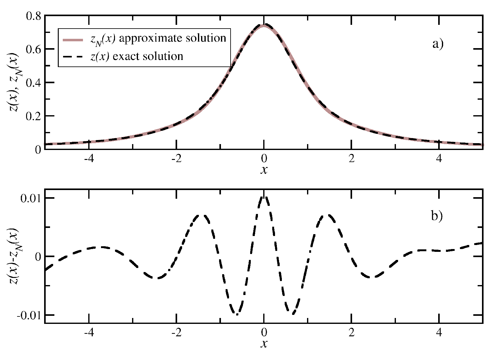
In Figure 1, we show a numerical example of solving Equation (49) using the NNH. In the works cited above, the NNH has been applied to nonlinear approximations of the original equation. Here, we demonstrate an application of the NNH to the original nonlinear equation with the logarithmic potential. Consider Equation (49) with the following parameters: $a=-5,b=5,G=1,\sigma \left(s\right)=1,H=2,f\left(x\right)=\underset{-5}{\overset{5}{\int }}ln({(x-s)}^2+4)ds-\underset{-5}{\overset{5}{\int }}ln({(x-s)}^2+{(2-3{(s^2+1)}^{-1}/4)}^2)ds$. The exact solution reads $z\left(x\right)=3{(x^2+1)}^{-1}/4$. Equation (49) has been solved numerically by solving the Cauchy problem for the following system of nonlinear differential equations

$$\frac{d{\alpha }_k\left(t\right)}{dt}=\frac{10}{N}{\displaystyle \sum _{l=0}^{N-1}}ln\frac{{(t_k-t_l)}^2+H^2}{{(t_k-t_l)}^2+{(H-{\alpha }_l\left(t_k\right))}^2}+f\left(t_k\right),k=0,1,\dots ,N-1,$$

where $t_k=-5+10k/N$ and the initial state ${\alpha }_k\left(0\right)=0.01$. The system has been solved by Euler’s method with time step $h=0.4$. In Figure 1a, we show the final state for N = 180 after 100 iterations together with the exact solution. The numerical and the exact solutions are indistinguishable in the scale of the figure. The corresponding numerical error is shown in Figure 1b.

10. Implementation and Numerical Experiments

We noted above that the continuous operator method has been applied for solving inverse coefficients problems [49], hypersingular integral equations [38], and inverse problems in astrophysics [50]. In each of these works, the obtained results were compared with the known ones.

The most significant advantages of the continuous method for solving nonlinear operator equations compared with iterative methods are as follows:

(1) Implementation of the basic method does not require Gateaux or Frechet derivatives of the operator to solve the equation; (2) Implementation of the modified method does not require invertibility of the Gateaux or Frechet derivatives of the operator to solve the equation; (3) The operator continuous method is based on Lyapunov’s stability theory for solving differential equations. The method is stable for coefficient perturbations in right-hand sides of equations.

In this section, the method’s efficiency is illustrated on the example of solving inverse problems for logarithmic potential. Hereby, we solve the exact equation without any simplifications. As far as the authors know, the inverse problem for logarithmic potential has not been previously solved in such a formulation.

Let us return to Equation (49) and write it in a more convenient form:

$$G\underset{0}{\overset{1}{\int }}\sigma \left(s\right)ln\frac{{(x-s)}^2+H^2}{{(x-s)}^2+{(H-u\left(s\right))}^2}ds=f\left(x\right),$$

(56)

where $u\left(s\right)$ is the function describing the surface of the body; $\sigma \left(s\right)$ is the density of the body, and H is the occurrence depth of the body.

Recall the issue. There is a gravitating body infinitely extended along the Y-axis and homogeneous along y. In this case, it can be treated as two-dimensional and we restrict ourselves to considering $y=0.$ Thus, we consider a body lying in the region $G:H-u\left(x\right)\le z\le H,0\le x\le 1.$ Let $f\left(x\right),0\le x\le 1$ stand for perturbation of the Earth’s external field. It is required to restore the function $u\left(x\right)$ given data about $H,\sigma \left(x\right),f\left(x\right).$

Similar problems are of great practical importance.

It was mentioned above that there are extensive studies devoted to the study of equations of the form (56). They considered either linearized equations or nonlinear approximations of Equation (56).

Below we demonstrate Hopfield neural networks for solving the original Equation (56).

Let ${\Delta }_k, k=0,1,\dots ,N-1$, and ${\Delta }_k=[t_k,t_{k+1}], k=0,1,\dots ,N-1,$ ${\Delta }_{N-1}=[t_{N-1},t_N].$ Here, $t_k=k/N, k=0,1,\dots ,N.$ Introduce the nodes ${\overline{t}}_k=(k+1/2)/N, k=0,1,\dots ,N-1.$

We will seek an approximate solution in the form of a piecewise constant function

$$u_N\left(x\right)={\displaystyle \sum _{k=0}^{N-1}}{\alpha }_k{\psi }_k\left(x\right),$$

where

$${\psi }_k\left(x\right)=\left\{\begin{array}{c}1,x\in {\Delta }_k,\hfill \\ 0,x\in [0,1]\backslash {\Delta }_k,\hfill \\ k=0,1,\dots ,N-1.\hfill \end{array}\right.$$

The coefficients ${\alpha }_k, k=0,1,\dots ,N-1$ are determined from the system of nonlinear algebraic equations

$$\frac{G}{N}{\displaystyle \sum _{l=0}^{N-1}}\sigma \left({\overline{t}}_l\right)ln\frac{{({\overline{t}}_k-{\overline{t}}_l)}^2+H^2}{{({\overline{t}}_k-{\overline{t}}_l)}^2+(H-u_N{\left({\overline{t}}_l\right)}^2)}=f\left({\overline{t}}_k\right),k=0,1,\dots ,N-1.$$

(57)

The system of Equation (57) is associated with the Cauchy problem

$$\frac{d{\alpha }_k\left(v\right)}{dv}={\gamma }_k(\frac{G}{N}{\displaystyle \sum _{l=0}^{N-1}}\sigma \left({\overline{t}}_l\right)ln\frac{{({\overline{t}}_k-{\overline{t}}_l)}^2+H^2}{{({\overline{t}}_k-{\overline{t}}_l)}^2+{(H-{\alpha }_l\left(v\right))}^2}-f\left({\overline{t}}_k\right)),k=0,1,\dots ,N-1.$$

(58)

The coefficients ${\alpha }_k=\pm 1, k=0,1,\dots ,N-1$ are selected so that the logarithmic norm of the Jacobian of the right side of the system (58) is negative.

The system (58) can be solved by any numerical method.

Application of the Euler method leads to the iterative scheme

$${\alpha }_k(m+1)={\alpha }_k\left(m\right)+h{\gamma }_k(\frac{G}{N}{\displaystyle \sum _{l=0}^{N-1}}\sigma \left({\overline{t}}_l\right)ln\frac{{({\overline{t}}_k-{\overline{t}}_l)}^2+H^2}{{({\overline{t}}_k-{\overline{t}}_l)}^2+(H-{\alpha }_l\left(m\right)){)}^2}-f\left({\overline{t}}_k\right)),$$

(59)

$k=0,1,\dots ,N-1$. Here, h is the step of the Euler method.

The algorithm described above was applied to solve the problem of restoring a gravitating body with the data: $\sigma =2, H=1.5, N=180, h=0.4, m=100.$

The exact solution of the problem is $u\left(x\right)=3/\left(2H(x^2+1)\right).$ The function $f\left(x\right)$ has been computed by the quadrature rule

$$f\left({\overline{t}}_k\right)=\frac{2}{N}\sum _{l=0}N-1ln\frac{{({\overline{t}}_k-{\overline{t}}_l)}^2+H^2}{{({\overline{t}}_k-{\overline{t}}_l)}^2+{(H-u\left({\overline{t}}_l\right))}^2}.$$

Detailed computational results are shown in

Table 2. Convergence of the continuous method to solution of nonlinear integral Equation (56) by a number of iterations, ${ϵ}_k=|u\left(t_k\right)-U_N\left(t_k\right)|$.

${\mathit{t}}_{\mathit{k}}$	${\mathit{U}}_{\mathit{N}}\left({\mathit{t}}_{\mathit{k}}\right)$	$\mathit{u}\left({\mathit{t}}_{\mathit{k}}\right)$	${\mathit{ϵ}}_{\mathit{k}}$
0	5.011124 × 10${}^{-1}$	5.000000 × 10${}^{-1}$	1.112496 × 10${}^{-3}$
1	5.065099 × 10${}^{-1}$	5.055864 × 10${}^{-1}$	9.235025 × 10${}^{-4}$
10	5.582226 × 10${}^{-1}$	5.586206 × 10${}^{-1}$	3.980314 × 10${}^{-4}$
20	6.220347 × 10${}^{-1}$	6.230769 × 10${}^{-1}$	1.042146 × 10${}^{-3}$
30	6.913298 × 10${}^{-1}$	6.923077 × 10${}^{-1}$	9.778526 × 10${}^{-4}$
40	7.635971 × 10${}^{-1}$	7.641509 × 10${}^{-1}$	5.537315 × 10${}^{-4}$
50	8.349188 × 10${}^{-1}$	8.350515 × 10${}^{-1}$	1.326703 × 10${}^{-4}$
60	9.000700 × 10${}^{-1}$	9.000000 × 10${}^{-1}$	7.007729 × 10${}^{-5}$
70	9.529645 × 10${}^{-1}$	9.529411 × 10${}^{-1}$	2.333060 × 10${}^{-5}$
80	9.876083 × 10${}^{-1}$	9.878048 × 10${}^{-1}$	1.965277 × 10${}^{-4}$
90	9.995410 × 10${}^{-1}$	1.000000	4.589433 × 10${}^{-4}$
100	9.872545 × 10${}^{-1}$	9.878048 × 10${}^{-1}$	5.502841 × 10${}^{-4}$
110	9.527123 × 10${}^{-1}$	9.529411 × 10${}^{-1}$	2.287820 × 10${}^{-4}$
120	9.004980 × 10${}^{-1}$	8.999999 × 10${}^{-1}$	4.980633 × 10${}^{-4}$
130	8.361412 × 10${}^{-1}$	8.350515 × 10${}^{-1}$	1.089730 × 10${}^{-3}$
140	7.646853 × 10${}^{-1}$	7.641509 × 10${}^{-1}$	5.344244 × 10${}^{-4}$
150	6.900979 × 10${}^{-1}$	6.923077 × 10${}^{-1}$	2.209774 × 10${}^{-3}$
160	6.153842 × 10${}^{-1}$	6.230769 × 10${}^{-1}$	7.692711 × 10${}^{-3}$
170	5.429360 × 10${}^{-1}$	5.586207 × 10${}^{-1}$	1.568470 × 10${}^{-2}$
180	4.747546 × 10${}^{-1}$	5.000000 × 10${}^{-1}$	2.524530 × 10${}^{-2}$

.

11. Conclusions

The paper is devoted to approximate methods for solving linear and nonlinear equations of mathematical physics. In doing so, we used a spline-collocation method based on a continuous method for solving nonlinear operator equations [19]. It has been shown that a continuous method computational scheme for solving nonlinear operator equations can be implemented with Hopfield neural networks. The efficiency and flexibility of the approach has been shown by evaluating multiple integrals, and solving Fredholm integral equations and hypersingular integral equations. In addition to the listed examples, the method was efficiently applied to a direct and inverse electromagnetic wave scattering problem [51], amplitude-phase problem [52,53], solving Ambartsumian’s systems of equations (astrophysics) [50], solving inverse problems of gravity and magnetic prospecting [47], and solving direct and inverse problems for parabolic and hyperbolic equations [54].

The authors intend to continue the study of the applicability of the continuous method for solving nonlinear operator equations, Hopfield neural networks, to new classes of equations. First, we want to use it for solving inverse problems in optics. Two points should be taken into account. First, the authors started to study the amplitude-phase problem [52,53]. Second, a couple of works devoted to applications of neural networks for inverse problems of restoration have been published recently [55,56]. It is of interest to investigate the possible use of the continuous operator method application for these issues.

As noted above, the continuous method for solving nonlinear operator equations is based on Lyapunov’s stability theory. The authors have studied the stability of Hopfield neural networks [22,57] and considered some issues of stabilization for dynamic systems [58,59]. A new statement of the problem of stabilization for dynamical systems was given in [60,61]. The authors intend to use this formulation in coming works.