1. Introduction
With the rapid development of the economy, people’s living standards have been significantly improved. Because the automobile is the main travel tool, its sales and users are gradually increasing. However, due to the impact of the decline of macroeconomic growth, China’s automobile industry is facing greater pressure in recent years. In 2019, the annual automobile sale was 25.769 million, down 8.2% year on year. Since 2020, due to the COVID-19 epidemic, the fixed asset investment of the automobile manufacturing industry has decreased significantly compared with the same period last year [
1]. Facing the changeable market and fierce competition, the accurate prediction of automobile sales is helpful for manufacturers to plan for procurement, production distribution and other links, so as to avoid asset losses and asset depreciation caused by overstocking. For retailers, dividing the annual sales target to each month and making reasonable sales plan in advance can reduce inventory cost and improve efficiency. Therefore, numerous scholars focus on the influencing factors and prediction methods of sales, which have an important guiding significance for the market development.
With the rapid development of the Internet and big data, a large amount of information from consumer behavior data, such as search trend data, online review data, star rating and so on, have become important resources for enterprises and researchers to predict product demand and supply. Therefore, more and more studies use consumer behavior data to make predictions in different fields. There are many explanatory research on product sales. Kostyra et al. [
2] studied the relationship between e-book reader sales and online reviews, and found that a higher star rating leads to higher selection probability. Kulkarni et al. [
3] found that the network search before the movie release follows certain rules, and the model integrated with the network search can significantly improve the prediction accuracy of the opening week box office. Li et al. [
4] used log linear regression to explore the relationship between computer sales and valence and word-of-mouth emotional scores and found that valence played a moderating role in the effect of emotion on sales. Wang et al. [
5] discussed the joint impact of competitive behavior and social media interaction on offline car sales after automobile recall. Conversely, there is considerable predictive research on product sales. Hu et al. [
6] proposed an ISCA-BPNN hybrid model based on a Google trend to predict the opening price direction and the future financial return. Li et al. [
7] and Liu et al. [
8] combined the technical indexes of stock prices with the text sentiment in news articles and the user information in social media platforms to predict stock price. Prasanth et al. [
9] used COVID-19-related Google trends and transmission data to predict future infections. Ai et al. [
10] effectively improved the prediction of tourist flow by introducing the Baidu index and the social media data on Twitter. Fan et al. [
11] used the Bass diffusion model to replace the model coefficient in innovation diffusion with text emotion value to effectively predict automobile sales. It can be seen that consumer behavior data have been widely used and have shown good performance in many product sales forecast problems, such as movie box office [
12], travel demand [
13], financial market [
14], etc.
The automobile is a kind of product with high value and high involvement. In the process of purchase, consumers need to have a comprehensive understanding of the ideal model in advance. The channels to collect such information include: physical stores, product manuals, networks, professional forums and so on. However, as automobile manufacturers, it only shows its advantages to consumers in publicity, which can lead to information asymmetry and make it difficult for consumers to obtain first-hand experience. At this time, online word-of-mouth data are a good reference. Through the analysis of the existing automobile forums, we find that every comment has a star rating given by consumers for different attributes of the automobile. The star rating from consumers can clearly reflect consumers’ feelings and objective evaluation of the car, which are useful for predicting automobile sales.
According to the existing literature, the main methods of sales forecasting include time series method, linear regression, machine learning method, grey forecasting method and so on. In the field of automobile sales prediction, autoregressive moving average and grey prediction are common forecasting methods. Shakti et al. [
15] used the autoregressive integrated moving average (ARIMA) model to predict the trend of automobile sales. Considering the influence of non-linear and non-stationary line on automobile sales, Sa-ngasoongsong et al. [
16] used the statistical unit root, weak exogenous, granger causality and hull cointegration test to identify the dynamic coupling relationship between sales and economic indicators, and they established the vector error correction model for multi-model automobile sales. Konstantakis et al. [
17] established a vector autoregressive model to predict automobile sales in Greece and estimated the long-term impact of different variables on automobile sales through generalized impulse response function. Furthermore, Ding and Li [
18] proposed an adaptive optimized grey model to predict the sales of electric vehicles and generated a dynamic weighted sequence to highlight the new data without information omission. To predict the sales of new energy vehicles in China, He et al. [
19] proposed an optimized grey buffer operator by introducing the cumulative translation transformation and determined its optimal parameters by genetic algorithm. Ding et al. [
20] proposed an adaptive data pre-processing and optimized nonlinear grey Bernoulli model to predict the sales of new energy vehicles and demonstrated the great forecasting accuracy of this model.
Through the analysis of the existing automobile market, it can be found that the automobile sales data present an obvious non-linear trend of change. The main influencing factors of automobile sales include social factors such as word-of-mouth reviews, Internet search index, consumer confidence index, and other self attributes such as car color, material, and price. In addition, the external environment such as economy, raw materials and policies can also affect the automobile sales to a certain extent. It can be seen that the automobile sales are affected by multiple factors. However, the traditional prediction model cannot handle the multi-source information and identify the nonlinear relationship well; thus, the prediction research based on machine learning is gradually enriched.
With the in-depth study of machine learning, its advantages in prediction problems gradually appear; thus, more and more scholars tend to use machine learning methods for prediction. The commonly used methods are artificial neural network (ANN), random forest (RF), support vector machine (SVM) and support vector regression (SVR). Chen et al. [
21] proposed a hybrid model combining extreme gradient boosting (XGBoost) and improved the firefly algorithm to predict stock prices. Vijh et al. [
22] used ANN and RF technology to predict the next day closing prices of companies in different industries. Peng and Xiang [
23] proposed a traffic flow prediction model using a genetic algorithm (GA) to optimize the back propagation neural network (BPNN). Yang et al. [
24] proposed a simulated annealing optimization ARIMA-BPNN model to predict network traffic, and the experiment results verified the effectiveness of the method. It can be seen that the machine learning method has been widely used in different fields for prediction problems, and it can improve the prediction performance of the model to a certain extent. However, because the automobile sales are mainly time series data, the research on this aspect is less. This paper attempts to use machine learning methods to predict automobile sales, which can not only explore the advantages of these methods in the automobile prediction problem, but can also provide more method selection and opinion reference for relevant researchers.
Since the SVR algorithm can easily avoid falling into a local optimum and has good generalization performance, many scholars are currently using the SVR algorithm for prediction research. To deal with the impact of model parameters on prediction performance, some meta-heuristic algorithms have been used to find the best parameters of the SVR model. For example, Liu et al. [
25] proposed a PM2.5 level prediction model based on particle swarm optimization (PSO) and SVR, and generated the better prediction accuracy. Many novel and efficient meta-heuristic algorithms have been proposed. In 2014, Mirjalili and Mirjalili [
26] proposed the Grey Wolf Optimization (GWO) algorithm, which can provide competitive results compared to well-known meta-heuristics, such as PSO, GA, Gravitational Search Algorithm [
27], Differential Evolution [
28], Evolutionary Programming [
29], and Evolution Strategy [
30]. In [
31], the GWO algorithm was applied to geophysical observation data, and the results show that the GWO algorithm takes the least time and produces more stable results than algorithms such as PSO and ant colony optimization [
32]. The GWO algorithm has the characteristics of strong convergence, fewer parameters and easy implementation; thus, it has attracted the attention of many scholars [
33]. Recently, the hybrid models of SVR and GWO methods have been wildly studied. Zhu [
34] performed NO2 and SO2 forecasting for cities in central China by building the SVR-GWO model. Rahmati [
35] proposed a hybrid model combining Wavelet-SVR-GWO for urban flood susceptibility mapping and demonstrated its superiority versus the single SVR method. These studies have demonstrated the excellent predictive performance of the SVR-GWO model.
According to the preceding analysis, the motivations of this paper can be summarized as follows. First, the prediction of automobile sales is mainly based on historical sales, the Baidu index, and the Google index, but there is little research considering online public praise. Therefore, this paper uses consumer star rating data to explore the role of user emotion in automobile sales prediction. Second, a large number of studies about sales prediction are for the whole market or are for annual sales prediction, which are less instructive to consumers. Thus, this paper makes predictions for specific models or brands to provide more specific reference opinions. Third, in addition to the characteristics of the car itself, the related factors of the external environment, such as economic factors, price factors and raw materials factors can also impact automobile sales. It can be seen that the sample data sources are diverse, the data complexity is high, and the sales data contain strong volatility and non-linearity. Therefore, this article proposes the SVR-GWO prediction model that can accommodate multi-source data and capture the nonlinear changes of data, where the GWO algorithm is used to find the best parameters of the SVR model to improve is prediction performance.
This paper is structured as follows:
Section 2 introduces the methods used in this study.
Section 3 presents the prediction model of automobile sales used in this paper.
Section 4 conducts the practical application and comparative analyses.
Section 5 provides some implications for practice. Lastly,
Section 6 draws the conclusions.
2. Methods
This section introduces the SVR model and GWO algorithm used in this paper.
2.1. Grey Wolf Optimization Algorithms
The GWO Algorithm is a population intelligence optimization algorithm proposed by Mirjalili and Mirjalili [
26] in 2014. The algorithm is developed by the inspiration of the predatory and hunting strategy of grey wolves in nature. Grey wolves belong to the predators at the top of food chain and tend to live in groups. In a group, grey wolves follow a strong leadership hierarchy. The leader of the wolves is called
wolf. The second layer is
wolf, which follows
wolf, but also commands the other lower-level wolves. The third level is
wolf, which obeys
and
wolf, but controls the remaining levels of wolves. The last level is
wolf, which must obey the other layers. The process of GWO optimization mainly includes social hierarchy, tracking, surrounding and attacking prey:
(1) Social hierarchy: The wolf is considered as the most appropriate solution in the mathematics of grey wolf hierarchy. Then, the wolf is called the second suitable solution. The next appropriate solution is the wolf. The other species representing the furthest solution are the remaining wolves. Through the GWO algorithm, the hunting process is directed by the , , wolve, and the wolf should only take the same steps and obey the wolf’s priorities.
(2) Surrounding prey: When the grey wolf hunts, it will gradually approach and surround it. This behavior is expressed as:
where
and
represent the coefficient vector;
is the position vector of the prey;
is the position vector of the current grey wolf. The vector of
and
is determined as follows:
where
decreases from 2 to 1 in the iteration process.
and
are random vectors in [0, 1].
(3) Hunting: Groups usually are guided by
,
,
, as they gain more experience in locating prey. The remaining agents must follow the optimal position and modify their positions accordingly. The adjustment formula of position is as follows:
where
,
,
represent position vectors of
,
,
in the current population, respectively;
represents the position vector of the grey wolf;
,
,
represent the distance between the current candidate grey wolf and the optimal three wolves respectively. While
, the grey wolves try to spread out in various areas and search for prey; when
, wolves will focus their search on one or more areas of prey.
(4) Attacking prey: is a random vector between and decreases linearly in the iteration process. When on the interval , the next moment position of the search agent can be anywhere between the current position of the Wolf and the prey.
(5) Prey hunting: Grey wolves mainly rely on information of , , to find prey. They start to scatter to find out where the prey is, and then, they come together to attack the prey. The establishment of the team dispersion model enables GWO to conduct a global search by to keep its search agents away from prey. Another search coefficient of GWO is , which provides random weight for prey, which helps GWO to display random search behavior in the optimization process to avoid falling into the local optimum.
2.2. Support Vector Regression (SVR)
The basic idea of SVR is: for limited data, input data are transformed into high-dimensional space by nonlinear transformation, and the linear decision function is constructed to achieve linear regression. Taking two-dimensional data as an example, interval bands are constructed on both sides of the linear functions. For all points falling into the interval bands, no loss is calculated. Only those falling outside the interval band are included in the loss function. Finally, the model can be optimized by minimizing the width of the interval band and the total loss. Therefore, the sample points of SVR finally have only one class, and the optimal hyperplane it seeks is to minimize the total deviation of all sample points from the hyperplane.
(1) Optimal fitting function of SVR
To maximize the width
of the interval band, the fitting curve and the optimal fitting function are defined as follows:
The above equation can be understood as: while maximizing the width of the interval band, the number of sample points that do not satisfy the constraint should be as few as possible. Therefore, the insensitive loss function is introduced. When the prediction error is less than and the sample points fall into the interval band, the loss is not included; otherwise, the loss is included.
Lagrange multiplier is introduced to obtain the fitting curve equation:
where
is the kernel function of SVR, which can convert a low-dimensional linear regression into a high-dimensional linear regression.
It can be seen that the SVR introduces as the insensitive loss function into the optimal fitting function, so as to minimize the total deviation of the fitting curve of all sample points distance. The difference from the general linear regression equation lies in that the prediction points are allowed to fall outside the range of the fitting curve, and the tolerance to error is high.
(2) Structure of SVR model
The model structure of SVR is composed of a linear combination of
intermediate nodes, each node corresponding to a support vector. Therefore, multiple factor variables are allowed to be input, and the final prediction results can be output. The structure diagram is shown as
Figure 1.
(3) Parameter setting of SVR
(a) Kernel function selection and parameter setting. The performance of SVR depends largely on the choice of kernel function and its parameters. Some experiments show that different kernel functions and their parameter settings have great influence on the fitting results in the SVR regression model.
(b) Penalty parameter c is set. c can adjust the confidence range and empirical risk of the learning machine in the feature space. When the sum of the relaxation variables of all outliers is determined, the larger c is, the greater the loss of the objective function will be. However, if the value of the slack variable is too small, the phenomenon of overfitting will occur. On the contrary, when the value of c is small, the phenomenon of under-learning will occur. Therefore, penalty factor c controls the balance between regression error minimization and classification hyperplane and local interval maximization. How to select the appropriate value of c for the SVR regression model is an important research problem.
(4) Characteristics of SVR model
(a) Regression prediction for small sample data: its algorithm can realize conduction inference from efficient training samples to test the samples; thus, it can solve the optimal value in small samples.
(b) The unique global optimal solution: SVR algorithm is actually a convex quadratic optimization problem. Theoretically, the global optimal value can be obtained, so as to avoid falling into the dilemma of local optimal easily.
(c) Good generalization performance: SVR uses the kernel function to map nonlinear data to high-dimensional space and builds linear fitting curves to ensure good generalization ability of the model while avoiding the problem of dimension disaster.
3. Construction of Automobile Sales Prediction Model
The prediction of automobile sales plays an important role in the automobile industry. Accurate prediction enables companies to improve market performance, reduce profit losses, and plan production processes and marketing policies more effectively. Fierce competition, significant investment, and the demand to rapidly upgrade models characterize the automotive industry, making prediction a critical factor in the sales and production processes. Similar to other complex industries, it has a long product development cycle; thus, effective production planning requires accurate long-term sales prediction. Inaccurate prediction may lead to some negative consequences, such as oversupply or shortage of production, high cost of different labor activities, loss of manufacturer’s reputation, and even bankruptcy.
As automobiles are high-value products, consumers’ purchase decisions are not only affected by the attributes of automobiles such as price, appearance and historical sales, but also by external factors such as economy, policy and raw materials. Therefore, this paper proposes a multi-factor automobile sales prediction model to make the sales prediction more accurate. In practical applications, different sources of sample data lead to high data complexity, high volatility and strong non-linearity. Therefore, a model that can contain multi-source data and capture nonlinear data variation is needed. In recent years, SVR has shown excellent performance in many fields and has been successfully applied to the prediction of nonlinear systems. Therefore, in the face of multi-factor automobile sales problem, the SVR model with global optimization, simple structure, strong generalization ability and that is suitable for predicting multi-dimensional small sample data is used. The GWO algorithm constructs a nonlinear model with the optimal combination of parameters through parameter optimization. To improve the prediction performance of the model, the GWO algorithm is proposed to optimize the SVR model for automobile sales prediction.
3.1. Determination of Influencing Factors
As an important high-value product in life, automobile sales are affected by many factors in the complicated economic environment. In general, economic conditions, product prices and raw materials can have an impact on the monthly sales of automobiles. The specific factors are analyzed as follows:
(1) Economic factors
The experiment and intuitive experience show that there is a positive correlation between a country’s economic development level and automobile sales. The higher the economic level, the higher the consumers’ economic affordability will be. They can maintain a positive attitude toward the economy, so as to improve their consumption willingness and promote them to buy high-value products such as automobiles. As a macro-economic index, the consumer price index [
36] can not only reflect residents’ consumption and price affordability but can also better reflect the trend of automobile economic environment and economic cycle, which is conducive to analyzing the trend of automobile sales. Furthermore, the change of money supply [
37] can also directly affect economic activities and thus have a certain impact on the sales of products. Therefore, the consumer price index and money supply can be used as economic factors affecting automobile sales.
(2) Price factor
It can be seen from the law of commodity value that the increase in product price can reduce sales; thus, there is a close relationship between product price and sales. The price of cars mainly affects the cost of purchasing, using and maintaining the car. The rise and fall of the price can directly affect the purchase intention. Excessively high prices can restrict consumers’ purchase intention [
38]. In recent years, the downward trend of automobile prices has also greatly promoted the purchase rate of automobiles [
39]. Therefore, automobile price is the factor that directly affects automobile sales.
(3) Raw material factors
The iron and steel industry is one of the key industries in the modernization construction; it is also an indispensable raw material for automobile manufacturing. The development level of China’s iron and steel industry increases with the development of industrial technology, which makes a huge increase in steel production on the market. However, with the increase in investment, there appears to be a situation of overinvestment and overcapacity, which directly affect the development of the automobile manufacturing industry [
40]. In addition, rubber is the main raw material of vehicle tires, and rubber tires are an essential part of vehicle manufacturing and later sales. The fluctuation of its output will have great impact on vehicle sales [
41]. Furthermore, diesel production has a great impact on oil price, which can also cause variation in automobile sales to some extent [
41]. Therefore, we take steel production, rubber tire production and diesel production as raw material factors.
Based on the above analysis of influence factors, this section takes the consumer price index [
36,
37,
40] (
), money supply [
37] (
), automobile price [
38,
39] (
), steel output [
40] (
), rubber tire output [
41] (
) and diesel output [
41] (
) as the external factors affecting automobile sales, combined with consumer star rating data of power [
38] (
) and comfort [
38,
41] (
) as the characteristic factors of a multi-factor automobile sale prediction model.
3.1.1. Correlation Analysis of Influencing Factors
The factors that affect the sales of automobiles come from different aspects with uncertainties. For manufacturers, to more effectively improve sales, it is important to analyze the importance of various influencing factors, focusing on those factors that have a higher impact on sales.
In mathematical statistics, some methods of variance analysis are commonly used, but it usually assumed that sample data obey a certain probability distribution. In practical application, it is difficult to meet such conditions due to the influence of data complexity. When the sample data are relatively small, a statistical method is not suitable. In contrast, grey correlation analysis does not limit the sample size; thus, this paper selects grey correlation analysis to judge the degree of correlation between sales and influencing factors. Assuming that the automobile sales sequence is the reference sequence, is the comparison sequence, represents samples, indicates influencing factors. Then, the steps to calculate the grey correlation degree between the two series are as follows:
(1) Since the statistical units of influencing factors are different, a dimensionless treatment is carried out for them:
where
is the
i-th influencing factor.
and
are the maximum and minimum values of
, respectively.
(2) Calculate the correlation coefficient
between automobile sales and influencing factors:
where
and
represent the minimum and maximum difference between the two poles, respectively,
is the resolution factor.
(3) Calculate the comprehensive correlation degree
. Since there are
samples, it is necessary to measure the overall correlation and calculate the average value of these
correlation coefficients, as the final correlation degree:
3.2. Data Source and Pretreatment
3.2.1. Data Source
The data of external factors such as steel output and money supply are from the monthly data database on the website of the National Bureau of Statistics, and the monthly sales data of automobiles are from the website of the Owner’s Home. The original data in this article are from Suteng and Kaluola, starting in September 2012 and ending in December 2020, with a total of 100 observations.
3.2.2. Data Preprocessing
(1) Processing of outliers and vacancy values
By observing the time series diagram or scatter diagram of the monthly sales of automobile, we identify one outlier from Suteng and four outliers from Kaluola. The common methods to deal with outliers include direct elimination, smoothing, filling and average correction. Because the sample data of sales in this paper are monthly sales, the number is not large. If the outliers are directly removed, the sample data will be insufficient, which will affect the prediction accuracy. Therefore, this paper uses the average correction method to correct them. Let
be the data series of sales and
be the outlier, and the formula to fill it is as follows:
where
m is the number of outliers before and after
.
Furthermore, due to the imperfect of statistical policy or other reasons, there are some vacancy values in some influencing factor data. When the National Bureau of Statistics collects receipts, it is found that there are two lines of data: the cumulative value of this month and the monthly value of this month. What we need is the monthly value. However, in some years, the monthly value of January and February is empty, and the cumulative value of January is also empty. For such data, this paper subtracts the monthly value of March from the cumulative value of March to the cumulative value of the first two months, then allocates it to February in an average way, and then subtracts the monthly value of February from the cumulative value of February to obtain the monthly value of January. In addition, in some years, only the monthly value and cumulative value of January are missing. For such data, the monthly value of January can be obtained by directly subtracting the monthly value of February from the cumulative value of February.
(2) Numerical normalization
Due to the different meanings and units expressed by each influencing factor, the values of each factor differ greatly. To accelerate convergence and improve prediction accuracy, the data need to be normalized:
where
is an influencing factor that needs to be normalized,
and
are the maximum and minimum values of the influencing factor, respectively, and
is the value after normalization.
3.3. Construction of Multi-Factor Automobile Sales Prediction Model
3.3.1. SVR Automobile Sales Prediction Model
Through the analysis of previous studies, it can be found that most of them are multi-factor prediction model for the annual sales of automobile. However, due to the characteristics of rapid economic development and fast update iteration of automobile products, the guidance of annual sales prediction for manufactures and sellers is less and less. In contrast, fine-grained monthly sales can give timely reference according to the change of demand market. Therefore, the monthly automobile sales are predicted through multiple factors. Considering that the data are small and the feature dimension is high, the SVR model that can accurately capture the nonlinear relationship under the limited sample size is selected for prediction. The construction steps of the SVR monthly sales prediction model are as follows:
(1) Establishing automobile sales fitting curve
The data set that defines automobile sales and its influencing factors is
, and
is the prediction value of automobile sales. Then, the fitting curve equation between automobile sales volume and influencing factors is as follows:
where
is the nonlinear eigenfunction that maps the data set of influencing factors to the high-dimensional space
.
is the weight (weight value);
is the bias (threshold).
(2) Defining the optimal fitting function
The goal of the fitting function is to minimize the total deviation of all predicted points from the hyperplane; thus, the fitting function can be transformed into a convex quadratic programming problem:
When the error of the sales forecast is no more than , the SVR forecast is considered to be accurate, and the loss is not included. Conversely, if the error is greater than , the loss is the absolute error minus .
(3) Optimal fitting function conversion
In practical application, due to certain human errors or collection problems, there will be certain fitting errors; thus, the relaxation factors
and
are introduced. Then, the optimal fitting function can be converted into:
where
is the number of samples, and
is the penalty factor. The larger the sample is, the higher the attention to the total error in the whole optimization process will be.
(4) Solving the Optimal Fitting Function
To solve the optimal fitting function, Lagrange multipliers
and
are introduced to obtain:
Then, take the partial derivatives of the four Lagrange multipliers and set them as 0. Substituting them into the above equation, and dualizing the objective function, the final function can be obtained as follows:
where
represents the RBF kernel function.
(5) Solving the optimal fitting curve
The value of
can be calculated as:
Thus, the optimal fitting curve of automobile sales volume can be obtained as follows:
where
represents the RBF kernel function.
3.3.2. The Parameters of SVR Model Optimized by GWO Algorithm
SVR shows its superiority in solving practical problems of small-sample, high-dimensional and nonlinear data and is widely used in function fitting. However, for SVR, the selection of penalty parameter and kernel function has a direct impact on the accuracy of model learning. In previous studies, the GA and PSO algorithms were mostly used to optimize the parameters of the SVR model. However, these optimization algorithms either have slow convergence speed, complex parameter settings, or an easy to fall into local optimum. Therefore, this paper selects the GWO algorithm to optimize the parameters of the SVR model. The GWO algorithm has fewer parameters, strong global search ability and is easy to implement, and it controls the local search scope of the algorithm, which can balance the global search ability and local search ability.
Common kernel functions for SVR include:
- (1)
Linear kernel function: ;
- (2)
Multinomial kernel function: ;
- (3)
Gaussian kernel function (RBF): ;
- (4)
Sigmoid kernel function: .
The linear kernel has no parameters, the polynomial kernel has parameters , and , the RBF kernel has parameters , and the sigmoid kernel has parameters and . According to the prior knowledge of the data, when the number of samples is large, the model effect of RBF and Sigmoid kernel function is better, and the convergence is better than that of the polynomial kernel function. When the number of samples is small and the number of features is much larger than the number of samples, the linear kernel function can also achieve the performance of RBF. Therefore, it can be obtained. Regardless of the multiple features, small features, multiple samples, or small samples, the RBF kernel function has better model performance and strong nonlinear mapping ability. Thus, this paper chooses the RBF kernel function as the kernel function of the SVR training prediction model.
The prediction accuracy of SVR is affected by parameter and penalty parameter . To improve the prediction accuracy of the model, GWO is adopted to optimize the parameters of the SVR model. The specific steps are as follows:
- (1)
Data preprocessing. Handle outliers, fill in missing values, and normalize influencing factor data.
- (2)
Model construction and data set partition. SVR model is established, and samples of sales volume and influencing factors are divided into training set and test set according to the ratio of 8:2. Then, penalty parameter , kernel function parameter and training data set are passed to the GWO algorithm.
- (3)
Parameter initialization settings. The parameters of the GWO algorithm are set, including the number of grey wolf population N, the maximum number of iterations T and the number of parameters solved . Set the optimal value range of penalty parameter and kernel function parameter .
- (4)
Random grey wolf population is generated, and the individual position of each grey wolf is determined by the value of penalty parameter and kernel parameter .
- (5)
Calculate the corresponding fitness of each grey wolf and divide the grey wolf into four grades , , , according to the fitness value.
- (6)
Update the position of each grey wolf in the group. Then, the new fitness is compared with the fitness before iteration to retain the optimal fitness value.
- (7)
Determine whether the current number of iterations has reached the maximum number of iterations. If so, the iteration will be terminated and the global optimal value will be output; otherwise, it will jump to (5) and continue the parameter optimization.
- (8)
Output the position of the grey wolf; then, the optimal parameters and are obtained.
- (9)
The optimal solution obtained by the GWO algorithm is given to the SVR model, and the verification set data are retrained to obtain the fitting result of the automobile sales of SVR.
The construction process of the GWO-SVR model is shown in
Figure 2.
The pseudo-code of the GWO-SVR algorithm is shown below (Algorithm 1).
| Algorithm 1: The Pseudo-code of GWO-SVR algorithm |
Input: the number of grey wolf population , the maximum number of iterations , the number of parameters solved p, the optimal value range of penalty parameter , RBF kernel function parameter , and the data set .
Output: the optimal parameters and , the predicted value and the error value of SVR.
Initialize the grey wolf population
Initialize the fittest solution α, search coefficient and
call the SVR
Calculate the fitness of each search agent
= the best search agent
= the second search agent
= the third search agent
while (t < T)
for each search agent
Update the position of the current search agent by Equation (7)
end for
Update , and
call the SVR
Calculate the fitness of all search agents
Update , and
end while |
4. Experiment and Analysis
In this section, GWO-SVR multi-factor automobile sales prediction method is applied to Suteng and Kaluola.
4.1. Experimental Procedure
The specific process of the GWO-SVR automobile sales prediction experiment based on multiple factors is shown as follows:
- (1)
Obtain the monthly sales of Suteng and Kaluola between September 2012 and December 2020 from the website of Home of Car Owners. Obtain data of consumer price index, money supply, steel output and other influencing factors from the website of National Bureau of Statistics. Online word-of-mouth data for both automobiles and their prices are obtained from Autohome’s website, and then the monthly average price is calculated.
- (2)
Preprocess and normalize the data of obtained sales and influencing factors.
- (3)
Build the GWO-SVR model, set the parameters, and divide the sample data.
- (4)
Input the training set data into the model network for training, and then verify them with the test set by obtaining the predicted value, error value, MAPE and RMSE performance value.
- (5)
Conduct comparative analysis of the model.
4.2. Correlation Analysis of Influencing Factors
After the sales and influencing factor data obtained from the website of owner’s home and the National Bureau of Statistics, the grey correlation coefficient is calculated to judge the correlation between each influencing factor and automobile sales. Based on the method of calculating the grey correlation coefficient in
Section 3.1.1, we write a program in MATLAB to solve and obtain the grey correlation degree between the influencing factors of Suteng and Kaluola, which are shown in
Table 1 and
Table 2.
From
Table 1 and
Table 2, it can be seen that steel output and rubber tire output have the highest correlation with automobile sales. Steel as raw material for automobile production and rubber tire as auto parts are also closely related to automobile sales. With the growth of automobile sales, the consumption of steel and rubber tires will also continue to increase, thus driving the increase in their production. The correlation degree of money supply and consumer price index is also above 0.6. The higher the correlation degree is, the higher the consumption level of the residents is, and the higher the willingness and ability to consume cars is. Diesel oil production also has a correlation above 0.6. As the main consumable of automobiles, the more the output of diesel is, the more the consumption is, which shows that the usage and sales of automobile are also increasing. As the main index for consumers to measure when buying goods, the correlation degree of automobile price is above 0.6, which also has great impact on automobile sales.
To sum up, the correlation degree between the six external influencing factors selected in this paper with automobile sales is above 0.6, indicating that they are all related to automobile sales. Therefore, this section uses these six external influencing factors as well as the historical sales and the star rating of consumers to build a multi-factor automobile sales prediction model.
4.3. Experimental Results and Analysis
Based on the data of Suteng and Kaluola, the GWO-SVR model is used to predict the multi-factor automobile sales. MAPE and RMSE are used to evaluate the prediction performance of the model.
According to the structure of the GWO-SVR model, the program is written in Matlab 2020b. The specific model training process is as follows:
- (1)
Normalize the data to eliminate the influence of data dimension on the model and accelerate the model learning speed.
- (2)
The sample data set is divided according to the 8:2 ratio. The first 80% of the data is the training set and the last 20% of the data is the test set. In this paper, we use a one-step prediction approach, i.e., we predict the last 20% of the data based on the learning of the first 80% of the data.
- (3)
Set the parameters of the GWO algorithm, including the number of grey wolf population N = 35, the maximum number of iterations T = 500, and the number of parameters solved is 2. The optimization range of penalty parameter C and RBF kernel function parameter is set as [0.01, 100] and [0.001, 100], respectively.
- (4)
The initial value is given to the GWO algorithm to conduct iterative parameter optimization, and then the optimal parameters = 39.2730 and = 0.0032 are obtained.
- (5)
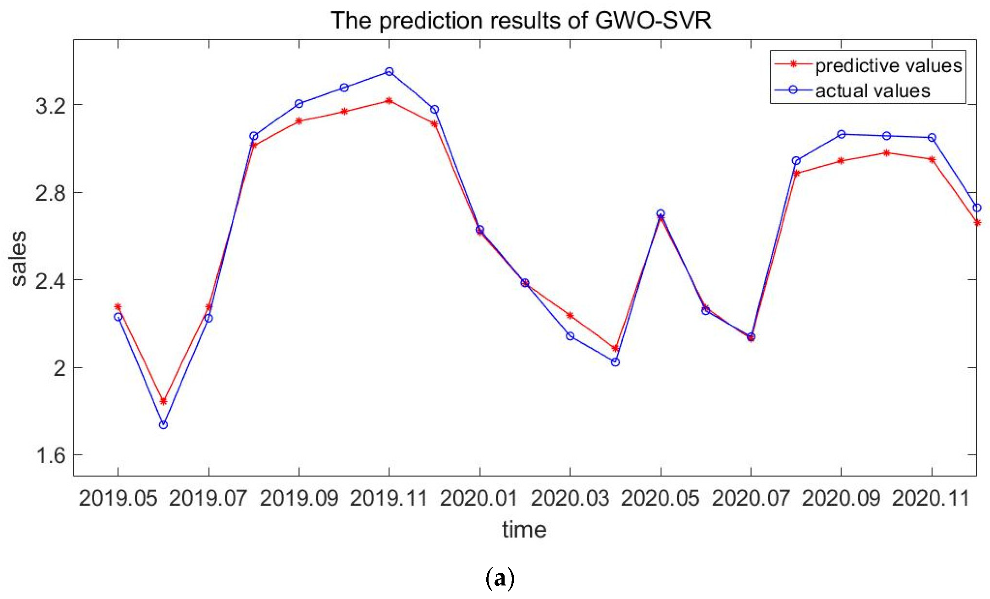
The parameters optimized by the GWO algorithm are transferred to the SVR model, and then the training and test set verification are carried out to obtain the predicted results and error values. The model fitting results of Suteng are shown in
Table 3 and
Figure 3.
It can be seen from
Table 3 and
Figure 3 that the prediction accuracy of Suteng based on the multi-factor GWO-SVR model is high, and the model fitting is good. The MAPE value is 0.0239 and the RMSE value is 0.0745, which are small. Thus, the multi-factor sales volume forecast improves the accuracy of the forecast.
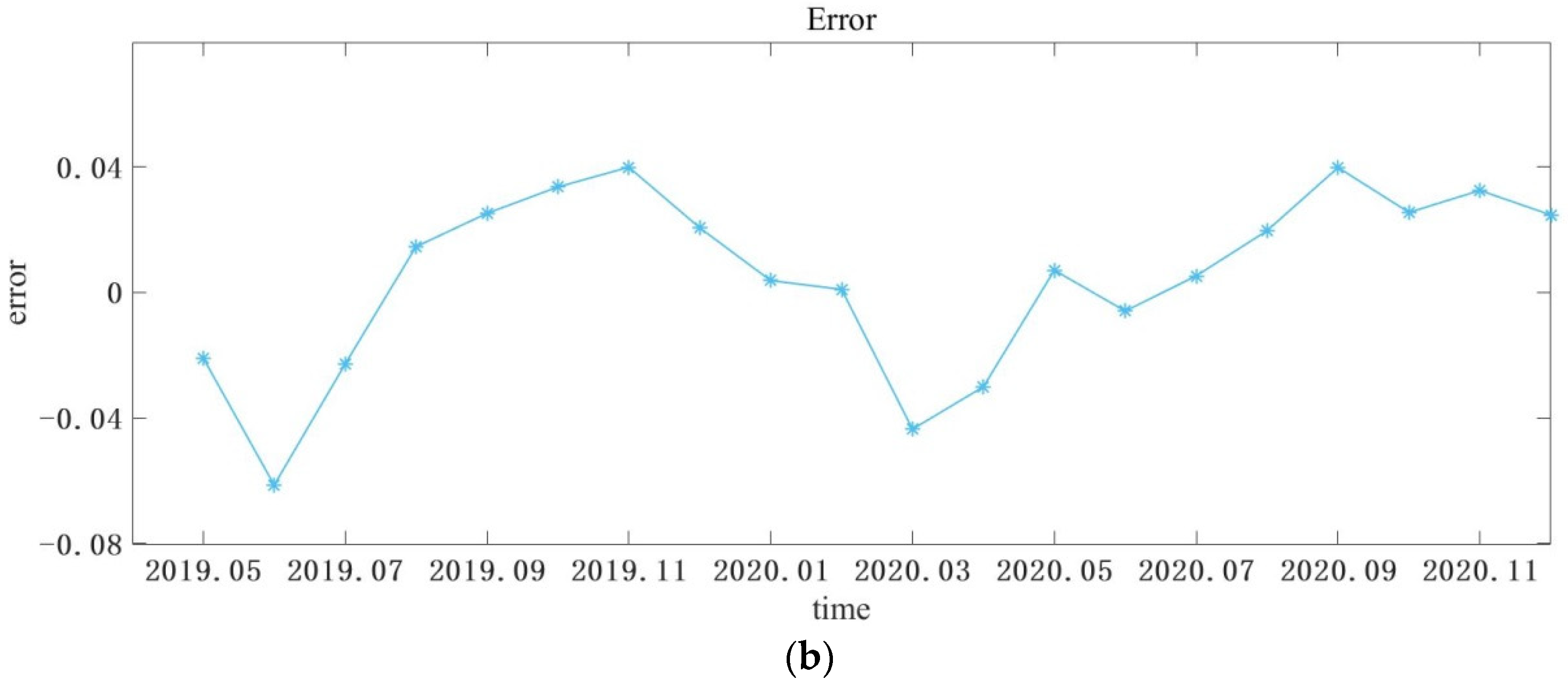
Similarly, according to the same model process, the fitting results of Corolla’s sales volume were obtained, which are shown in
Table 4 and
Figure 4.
It can be seen from
Table 4 and
Figure 4 that the experiment of the GWO-SVR model is conducted with Kaluola data, and the prediction results are good, with a MAPE value of 0.1419 and RMSE value of 0.5187. The SVR model is suitable for multi-dimensional and small sample data, which is in line with the characteristics of automobile sales data. In addition, the GWO algorithm is used to optimize the parameters of the SVR model to avoid the influence of parameters on the prediction accuracy of the model, thus improving the accuracy of the model.
4.4. Comparative Analysis of Models
To test the effectiveness and adaptability of the method presented in this paper, the GWO-SVR model was compared with the SVR model, PSO-SVR model, FA-SVR model and ABC-SVR model.
Comparative Experiment 1: Support Vector Regression Model for automobile Sales prediction Based on Multiple Factors—SVR
Since the parameters of SVR can affect the accuracy of the model, the first experiment compares GWO-SVR with the conventional SVR model to verify whether the GWO algorithm can improve the prediction performance of the model.
Comparative Experiment 2: Particle Swarm Optimization Algorithm Based on Multiple Factors—SVR automobile Sales Prediction Model—PSO-SVR
As a common global optimization algorithm, the PSO algorithm is also often used in parameter optimization, and many studies combine the PSO algorithm with SVR model. Therefore, the second experiment selected PSO-SVR for comparison to verify the applicability and superiority of the proposed model.
Comparative experiment 3: Artificial bee colony algorithm based on multiple factors—SVR automobile sales prediction model—ABC-SVR
The artificial bee colony algorithm can avoid falling into a local optimal solution to a large extent by imitating a bee colony for parameter optimization. At the same time, it has better optimization performance than a traditional optimization algorithm in dealing with multi-dimensional problems. It is also a widely used intelligent optimization algorithm; thus, it is taken as the third comparison model.
Comparative experiment 4: based on the multi-factor firefly algorithm—SVR automobile sales prediction model—FA-SVR
The firefly algorithm is a new random group search optimization algorithm, which simulates the process of attracting and moving fireflies when they flash. Different attraction models in FA have different fitness comparison numbers and attraction numbers. At the same time, the firefly algorithm has a faster convergence speed when solving the high-dimensional problems and can quickly obtain the results. Therefore, FA-SVR was used as the fourth comparison model.
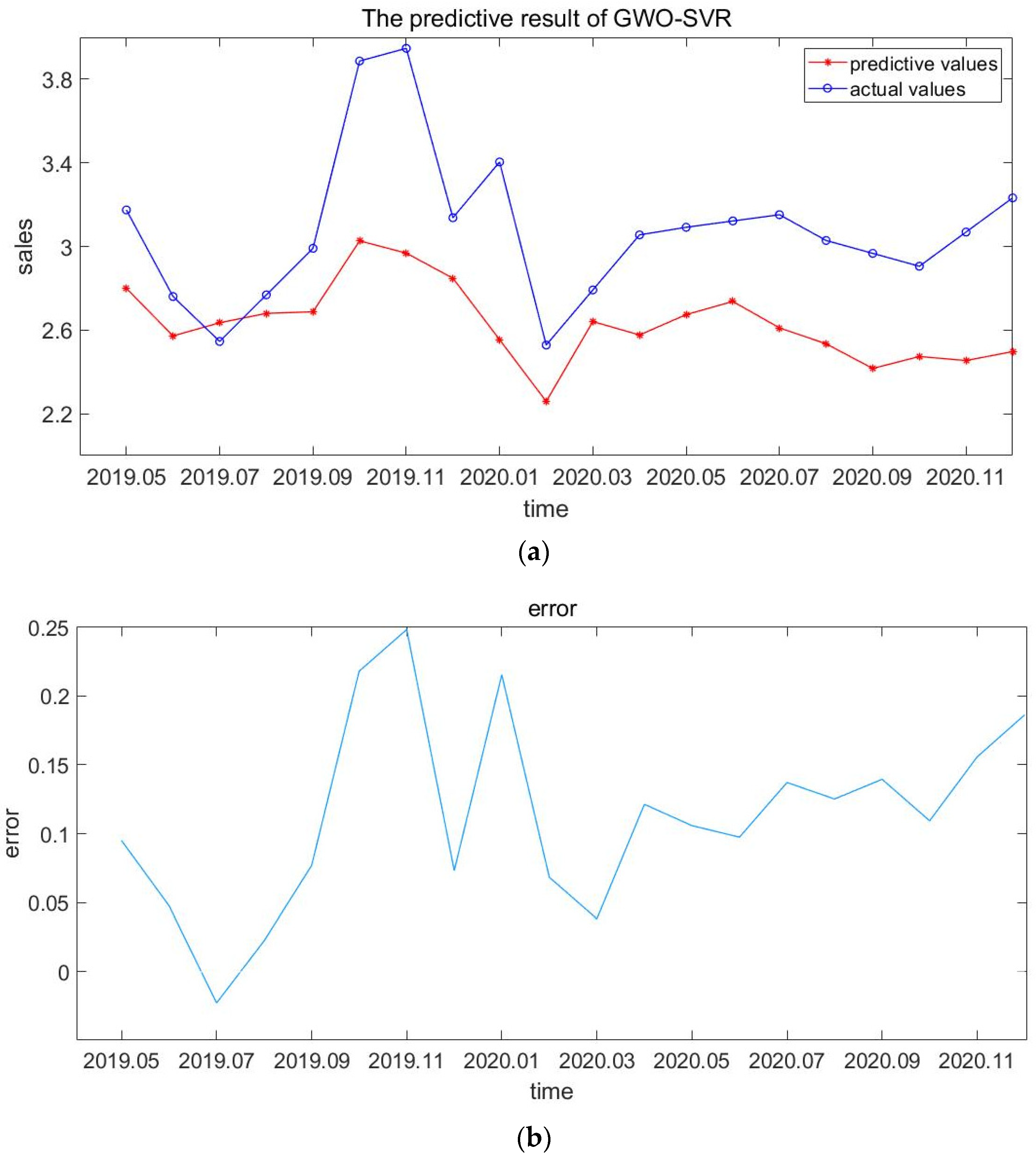
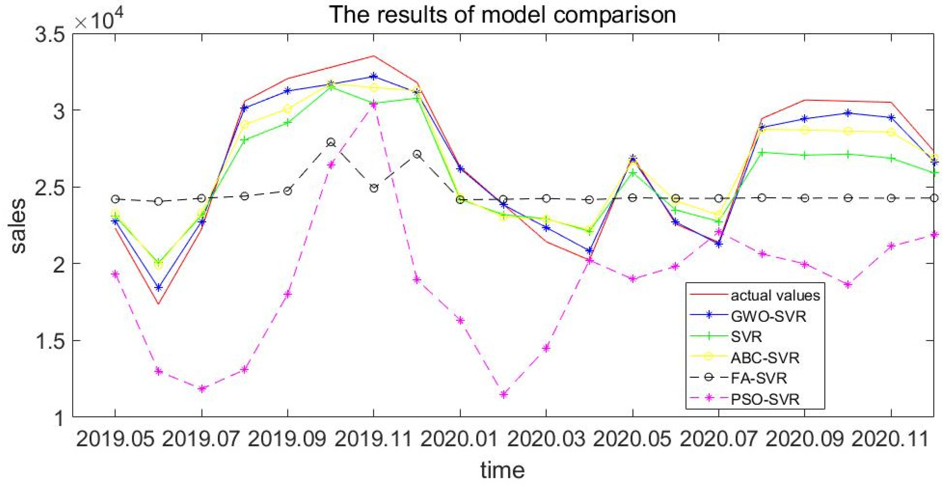
The four groups of comparative experiments selected the same training set and test set in this paper, and the comparative experimental results obtained are shown in
Table 5 and
Figure 5 and
Figure 6.
According to
Table 5,
Figure 5 and
Figure 6, the prediction accuracy of the GWO-SVR model is better than that of the other four comparison models when predicting the monthly sales of Suteng and Kaluola. The MAPE value of Suteng in the GWO-SVR model is 0.0239 is lower than that of SVR model (0.0728), PSO-SVR model (0.1120), ABC-SVR (0.07582) and FA-SVR (0.1619). The performance value of Kaluola in the GWO-SVR model is also significantly lower than that of the PSO-SVR, ABC-SVR and FA-SVR models, indicating that the prediction accuracy of the SVR model is improved after the optimization of the GWO algorithm. Compared with the basic SVR model, the GWO-SVR model optimizes the parameters through the GWO algorithm to avoid the influence of parameter problems on model performance. Compared with the PSO-SVR, ABC-SVR and FA-SVR models, the GWO algorithm can build a nonlinear model of input and output with optimal parameter combination through intelligent optimization, so as to achieve a balance between global and local search capabilities. In addition, the GWO algorithm has fewer parameters, is easy to implement, has a strong convergence performance, and improves the accuracy of the model.
Although the above experiments were carried out for Chinese conditions, foreign automobile sales are also affected by consumer star rating and multiple external factors as in China. Therefore, the proposed method is also applicable to foreign conditions. Furthermore, other new influence factors can also be added into the presented methodology, which reflect the universality of the method.
5. Some Implications for Practice
According to the prediction results of automobile sales, it can be found that in addition to star rating, other external factors can also have great impact on automobile sales. Therefore, apart from paying attention to factors of the car itself, automobile manufactures and sellers also need to pay attention to the social environment, and adjust policies and plans according to relevant policies in a timely manner. To ensure the healthy development of the market, this paper puts forward some suggestions:
(1) Adjust production and sales plans according to the policy environment in a timely manner.
Since automobile manufacturing and production take a long time and require many parts, it is necessary to carry out accurate market demand prediction. Then, we can make a reasonable lead time and inventory plan for parts to ensure that the market demand can be met. The complete supply chain, from suppliers and manufacturers to the final delivery of products to consumers, involves many members and takes a long time. Therefore, it is necessary to update the market demand data in time and share information in the whole supply chain, so that the production enterprises and sales enterprises can respond to market changes in time. This can avoid large-scale inventory backlog or product shortage.
(2) Respond to consumer demand in a timely manner, improve the quality of automobiles, and strengthen after-sales services.
At present, there are many consumers’ reputations on the Internet and automobile professional forums. Enterprises should pay attention to these data, dig deep into the problems and make timely improvements to these problems. This can improve the quality of their products. Conversely, it can also improve customer satisfaction. As the automobile is a high-value commodity, consumers not only pay attention to the quality of the car itself, but also pay great attention to the after-sales services. However, at present, some brands in the market lack the concept of the overall product, and service consciousness and ability are relatively low, which reduce customer satisfaction. Therefore, we must pay attention to strengthen after-sales services to improve the competitiveness of products in the market. First, we can improve the professional ability and quality of employees by training professional technical teams. Second, we can establish an interactive platform between enterprises and consumers to understand the problems and needs of consumers in a timely manner. Third, we can visit customers regularly and provide customers with some service such as fault trailer and vehicle maintenance.
6. Conclusions
In recent years, the Internet and artificial intelligence have developed rapidly, and some Internet word-of-mouth information in online platforms and forums can directly influence consumers’ purchasing decisions. Therefore, this paper proposes a multi-factor GWO-SVR automobile sales prediction model considering consumer star rating and external influencing factors. The SVR model has the advantages of global optimization, simple structure and strong generalization. The most important thing is that it is suitable for multi-dimensional and small sample data, which are in line with the characteristics of influencing factors and sales data. Therefore, the SVR model is used for model training. To avoid the influence of penalty factor and kernel function on model performance, the GWO algorithm is used to intelligently optimize the model parameters to improve model accuracy.
We used the data of Suteng and Kaluola for experiments and then took the MAPE and RMSE values as the performance evaluation indexes of the model. First, through a literature review, this paper summarizes the factors influencing automobile sales, and determines that steel output, rubber tire output, money supply, diesel output, consumer price index and automobile price are six external influencing factors. The grey correlation degree between them and automobile sales is greater than 0.6, which shows that they have an impact on sales. By inputting the data of Suteng and Kaluola into the model, the MAPE and RMSE of Suteng are 0.0239 and 0.0745, and the MAPE and RMSE of Kaluola are 0.1419 and 0.5187. The error is less than 10%, which shows great prediction accuracy. To test the validity of the model, the GWO-SVR model is compared with SVR, PSO-SVR, ABC-SVR and FA-SVR. The MAPE and RMSE values of the GWO-SVR model are the smallest among the five models, which indicates that the proposed model has good performance in multi-factor automobile sales prediction.
In view of the prediction problem of monthly automobile sales, this paper builds the GWO-SVR automobile sales prediction model based on multiple factors considering the star ratings of consumers in online forums, which is of great guiding significance for the automobile industry. However, there are still some shortcomings in the research, which need further study in the future.
(1) The online review data of consumers contain important emotional information of consumers. The sentiment analysis method can be used to mine the (feature, emotional value) pairs in the review data, so as to improve the prediction performance.
(2) With the rise of the deep learning algorithm, its superiority in the prediction problem has been verified. Therefore, we can consider the application of the deep learning algorithm in the automobile sales problem to improve prediction accuracy and efficiency. In addition, we need to explore the factors that affect automobile sales and pay attention to the correlation between the influencing factors. We can remove the correlation and reduce the dimension to verify whether the accuracy of the model can be further improved.


