A VIKOR-Based Linguistic Multi-Attribute Group Decision-Making Model in a Quantum Decision Scenario

Abstract

Quantum decision theory has been successfully applied to multi-attribute group decision-making (MAGDM) to model decision-makers’ interference and superposition effects in recent years. Existing quantum models assume that interference effects among decision-makers are symmetric. However, asymmetric interference effects have been ignored. We propose a VIKOR-based linguistic distribution assessments (LDAs) model considering asymmetric interference effects in a quantum decision scenario. Firstly, we combine VIKOR with LDAs to obtain a compromise solution in a fuzzy multi-attribute decision scenario with conflicting attributes. Secondly, an aggregation framework based on quantum probability theory is constructed to explore group preferences considering asymmetric interference effects among decision-makers. Finally, the model is compared with other methods to confirm its validity and stability.

1. Introduction

In the field of decision-making theory, multi-attribute group decision-making (MAGDM) is a significant branch, and its approaches [1,2,3] have been widely studied and applied in emergency decision-making [4], health systems [5], and supplier selection [6,7]. A typical MAGDM problem includes three aspects: a problem to be solved; several decision-makers with different backgrounds; obtainment of a common opinion from multiple decision-makers. In this section, we review the development of the related methods and put forward the problem that needs further study.

1.1. Literature Review

Along with the increasing complexity of decision-making environments in real decision scenarios and the limitations of human knowledge, preferences expressed by linguistic information are more acceptable and widely used. Linguistic information has been extended into diversified forms to accommodate various complex decisions, e.g., virtual linguistic term sets [8], probabilistic linguistic term sets (PLTSs) [9], 2-tuple linguistic model [10], hesitant fuzzy linguistic term sets (HFLTSs) [11], etc. The abovementioned linguistic models can depict individual linguistic evaluation well, but they cannot express group evaluations with numerous linguistic terms (LTs). Currently, group evaluations are becoming increasingly important in decision-making, particularly when customers are willing to seek advice on websites. In view of this situation, online platforms such as some travel websites (ctrip.com (accessed on 12 March 2022)) can also provide group evaluations in the form of linguistic distribution, such as, ‘85% of tourists think the destination is very good, 12% think it is moderate, and 3% think it is poor’. By understanding these linguistic distribution reviews, tourists can make better choices. Therefore, establishing a scientific expression model to gather group linguistic evaluations and integrally depict the quantitative distribution is essential.

The concept of linguistic distribution assessments (LDAs) was first proposed by Zhang et al. [12]. LDAs can make an overall summary of group linguistic assessment statistically. LDAs are feasible in describing qualitative and quantitative information both of individuals and groups, and they have been applied in various decision-making problems [12,13,14]. A group LDA usually should include three parts: LTs, probability distribution, and sample capacity information. The sample capacity information is significant for an LDA since the probability distribution is mainly determined by it. However, most of the previous research on group LDAs [13,14] ignored this key element, which is inappropriate. To address this issue, Wu et al. [15] proposed LDAs with sample capacity to ensure the objectivity of the probability distribution when dealing with a MAGDM problem. LDAs are commonly measured by distance measure. However, the previous distance measure of LDAs [14] is not applicable to calculate the difference of LDAs with sample capacity, so a new distance measure method is needed for this type of LDA.

It is important to choose an appropriate multi-attribute decision-making (MADM) method when solving a MAGDM problem. Different MADM models have their own characteristics. There is no MADM method that is superior to the others in all aspects. Hafezalkotob et al. [16] classified the MADM aggregation methods into three categories: value measure methods, outranking methods, and compromise methods. Value measure methods include Simple Additive Weighting (SAW) [17] and Weighted Aggregated Sum Product Assessment (WASPAS) [18], etc. Outranking methods mainly refer to Elimination and Choice Expressing the Reality (ELECTRE) [19], Preference Ranking Organization Method for Enrichment of Evaluations (PROMETHEE) [20], etc. Compromise methods incorporate TOPSIS (Technique for Order Performance by Similarity to Ideal Solution) [21], VlseKriterijumska Optimizacija I Kompromisno Resenje (VIKOR) [22], etc. In many real cases, attributes often conflict with each other. The VIKOR method, which was introduced by Opricovic [23], is a popular method to handle conflicting attributes to obtain compromise solutions. A comparison between the VIKOR method and other MADM methods also was carried out by Opricovic and Tzeng [24,25]. They showed some advantages of the VIKOR method. Furthermore, various extended forms of VIKOR methods have been developed, such as the hesitant fuzzy VIKOR [26], dual hesitant fuzzy VIKOR [27], hesitant fuzzy linguistic VIKOR [28], and interval type-2 fuzzy VIKOR [22], etc. However, the VIKOR method combined with LDAs with sample capacity has not been studied. This combination will be helpful to improve the accuracy of fuzzy decision-making.

Most existing group decision-making (GDM) models assume that the decision-makers make independent decisions, which is unreasonable in reality [29]. In the process of integrating individual results into a group decision result, the dependence of decision-makers in a MAGDM problem, which is also called the interference effects in quantum decision theory (QPT), has attracted growing concern. QPT can be used to construct dynamic systems [30,31], and it has been widely studied and applied in different fields, e.g., cognitive and human behavioral sciences [32,33], psychology [34,35], decision-making [36,37,38], and artificial quantum intelligence [36], etc. Many paradoxes can not be explained by classical probability theory (CPT): the Ellsberg paradox [39], the disjunction fallacy [40,41], the order effect [42,43], etc., can be well-explained in QPT framework. Some recent studies on cognitive psychology [44,45,46] verified that the quantum probability theory can develop a group decision model which can simulate the real decision-making process of human beings. They [44,45,46] believe that human thoughts can be regarded as superposition waves, thus the concept of “interference” emerged. Given the strong ability of the QPT framework to capture the intuitive feeling of uncertainty, ambiguity, or conflict, it is natural to extend it to deal with MAGDM problems [29]. However, the previous studies assumed that interference effects among decision-makers are symmetric. In other words, for different alternatives, the influence of opinion between decision-makers is equal. There is not enough evidence to prove that this assumption is correct. Therefore, MAGDM problems with respect to asymmetric interference effects deserve further study.

1.2. Motivations and Innovations

Through the above discussion and analysis, the main motivations of this paper include the following three aspects:

• Although LDAs with sample capacity can well-express group linguistic evaluation, the distance measure of LDAs in previous studies is not applicable to LDAs with sample capacity. Therefore, it is necessary to develop a new distance measure to compare LDAs with sample capacity.
• The problem of attributes conflict can be handled by VIKOR method; we try to extend VIKOR method to the context of LDAs. When considering the interaction of decision-makers in a group, how to reflect the group interaction relationship based on this method?
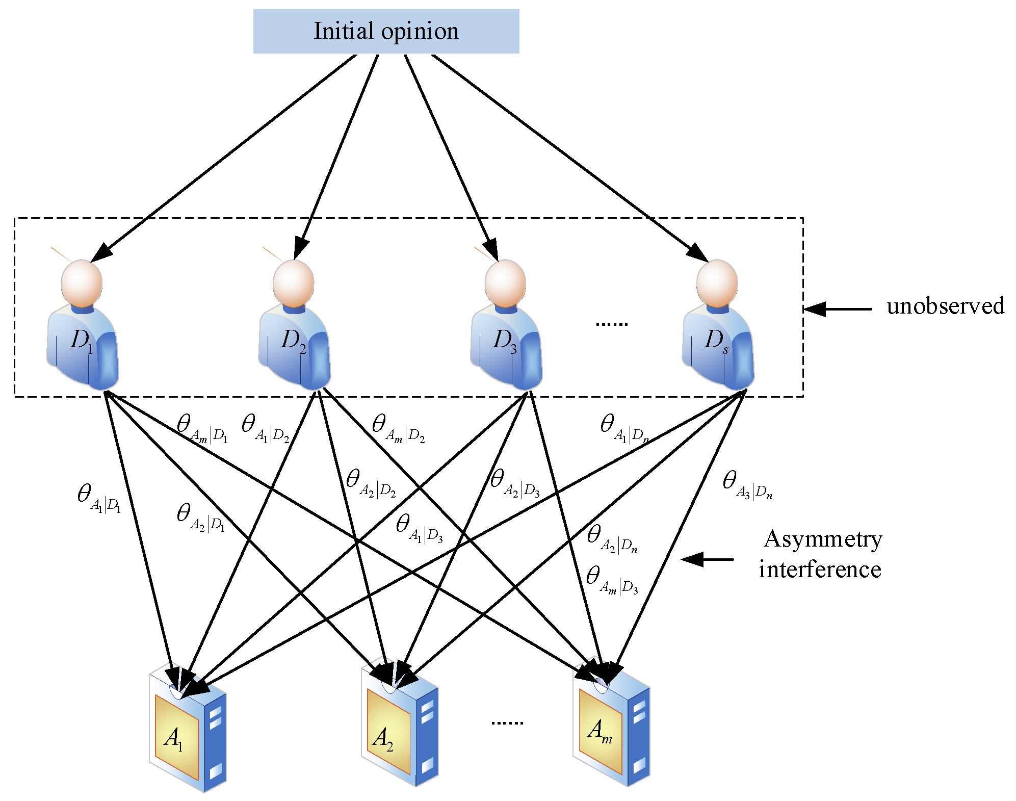
• In the process of dealing with MAGDM problems, it is necessary to consider the asymmetric influence among decision-makers when using QPT. Therefore, it is significant to explore the asymmetric interference effect in the quantum decision framework.

Hence, this paper develops a VIKOR-based linguistic MAGDM model in the quantum decision framework to obtain compromise results and reflect the dependency of decision-makers. The main innovations are as follows:

• A new distances measure is developed for LDAs, which can preserve the integrity of linguistic information.
• We propose an LDAs–VIKOR method to obtain a set of compromise results instead of a single result. It provides a new decision-making mechanism for decision-makers when circumstances are uncertain.
• We combine the QPT with the LDAs–VIKOR method to reflect the interaction among decision-makers. The asymmetric interference is proposed to describe the degree of interaction of a group in a more detailed and realistic manner.

The rest of this paper is arranged as follows. Section 2 introduces the concept of LDAs with sample capacity and QPT. Section 3 proposes the asymmetric interference effects among decision-makers in group decision-making (GDM) and verifies its rationality by formula derivation. Section 4 constructs an LADs-VIKOR model to solve the MAGDM problem in a quantum decision scenario. A case study is presented to validate the effectiveness of the proposed model in Section 5. The sensitivity and discussion display the flexibility of our model. Finally, advantages, limitations, and future studies are given in Section 6.

2. Preliminaries

In this section, we briefly introduce the basic concepts of LDAs with sample capacity, QPT, and the interference term. This section provides the basis for the following sections.

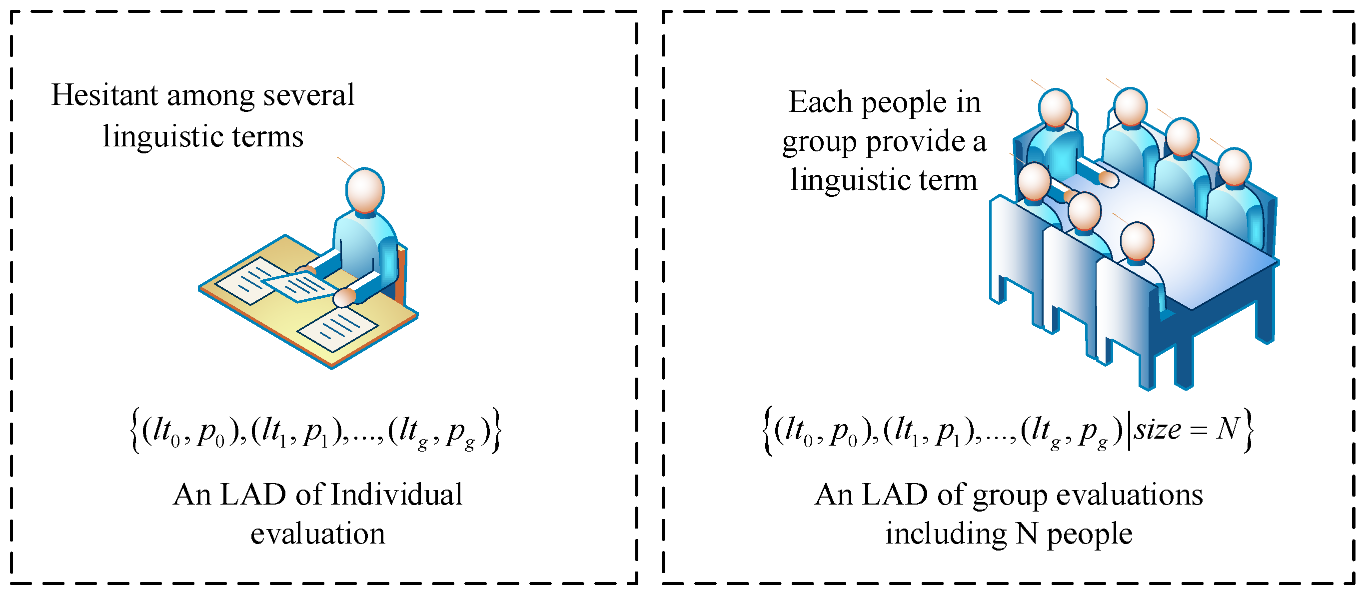
2.1. LDAs with Sample Capacity for Group Evaluations

LDAs are very common, and they can depict fuzzy information. As we know, there are two types of LDAs: “individual evaluations” and “group evaluations” (see Figure 1). In general, LDAs depend on a linguistic term set $L=\left\{l_v|v=0,\dots ,g\right\}$ which is pre-given. Individual evaluation refers to a decision-maker who is irresolute about several linguistic terms, then he/she can use LDA to express his/her opinion. Group evaluation mean that there are $N$ members in a group. Each member in the group provides only one linguistic term for the evaluation event. Then the $N$ evaluations given by $N$ members make up an LDA of group evaluation. Most LDAs are group evaluations, e.g., online reviews movie ratings, hotel rankings, etc. Thus, we concentrate on group evaluations of LDAs. Wu et al. [15] defined the concept of LDAs with sample capacity.

Definition 1 

[15]. Let $L=\left\{l{t}_v|v=0,\dots ,g\right\}$, an LDA is defined as: $T=\{\left(l{t}_v,p_v\right)|l{t}_v\in L,p_v\in \left[0,1\right],{\displaystyle \sum }_v{p}_v=1,size=N\}$, or $T=\{\left(l{t}_v,N_v\right)|l{t}_v\in L,N_v\in \left[0,N\right],{\displaystyle \sum }_v{N}_v=N,size=N\}$.where $N$ is the total sample capacity of the LDA, the term $\left(l{t}_v,p_v\right)$ and $\left(l{t}_v,N_v\right)$ are the probability$p_v$ and size $N_v$ with respect to the linguistic term $l{t}_v$.

Example 1.

Suppose a travel destination on Ctrip is rated by 68 tourists; 45 of them think it is “very good”, 15 of them think it is “good”, 5 of them think it is “moderate”, 3 of them think it is “bad”, and none of them think it is “very bad”. These linguistic evaluations can be summarized into an LDA: $T=\left\{\left(l{t}_0,45/68\right),\left(l{t}_1,15/68\right),\left(l{t}_2,5/68\right),\left(l{t}_3,3/68\right),\left(l{t}_4,0/68\right)|N=68\right\}$, where $\left\{l{t}_0,l{t}_1,l{t}_2,l{t}_3,l{t}_4\right\}$corresponds to the linguistic terms $\left\{very bad,bad,moderate,good,very good\right\}$.

Figure 1. The difference between individual evaluation and group evaluation of LDA [15].

LDAs are equal if their values of expected utility are same [12]. Hence the comparison of LDAs can be defined as follow:

Definition 2 (Score function)

[15]. Let $T=\{\left(l{t}_v,p_v\right)|l{t}_v\in L,p_v\in \left[0, 1\right],{\displaystyle \sum }_t{p}_v=1,size=N\}$ be an LDA, the score function of $T$ is given as:

$$E\left(T\right)=\frac{1}{g+1}{{\displaystyle \sum }}_{v=0}^g{p}_v·f\left(l{t}_v\right)$$

(1)

where $g+1$ is the total number of $L$, $v=\left(0,1,2,\dots g\right)$. $f$is the linguistic scale function.

According to the score function (expected utility function), for any two LDAs$T_1$and$T_2$, we can conclude that [15]:

(1)

If$E\left(T_1\right)>E\left(T_2\right)$, then$T_1\succ T_2$;

(2)

If$E\left(T_1\right)<E\left(T_2\right)$, then$T_1\prec T_2$;

(3)

If$E\left(T_1\right)=E\left(T_2\right)$, then$T_1~T_2$.

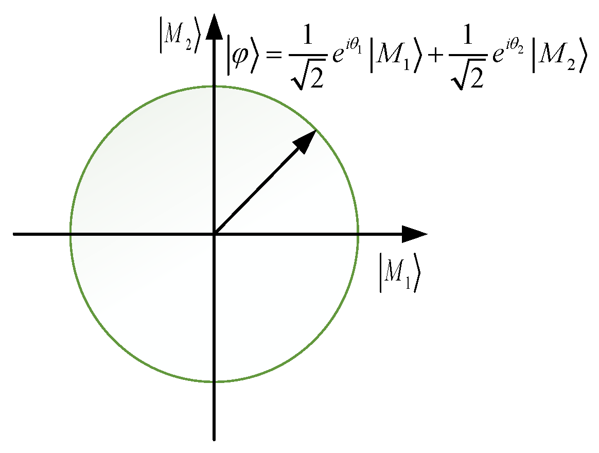
2.2. Quantum Probability Theory (QPT) and the Interference Term

In the framework of CPT, the events are subspaces of sample space $\mathsf{\Phi }$, while in QPT, the events are regarded as subspaces of the Hilbert space, which are mutually exclusive or related [29]. Take an event with two basic states $\mathsf{\Omega }=\left\{M_1, M_2\right\}$ as an example: the Hilbert space consists of a set of orthonormal basis vectors, which can be written by: $|\psi ⟩={\phi }_{1}exp\left(i{\theta }_1\right)|M_1⟩+{\phi }_{2}exp\left(i{\theta }_2\right)|M_2⟩$, where $|M_1⟩$ = (1,0), $|M_2⟩$ = (0,1).

Hilbert space of two-dimensional quantum probability is shown in Figure 2.

Figure 2. An example of quantum probability in two dimensions.

According to Born’s rule [47], the square of the probability amplitude equals to the classical probability [48]. So, the conversion relationship between probability amplitude and classical probability is:

$$P(M_1)={\left|{\phi }_1\exp \left(i{\theta }_1\right)\right|}^2={\phi }_1{}^2, P(M_2)={\left|{\phi }_2\exp \left(i{\theta }_2\right)\right|}^2={\phi }_2{}^2$$

(2)

where $P(M_i)$ is the classical probability of state $M_i$.

A path graph is usually used to represent the dependency of a set of variables. Busemeyer et al. [49] firstly proposed an experimental study of the decision process by comparing Markov and quantum model. By using conditional probabilities, the probability of single path $P\left(X\to M\to Y\right)$ is given by:

$$P\left(X\to M\to Y\right)=P\left(X\right)·P\left(M|X\right)·P\left(Y|M\right)$$

(3)

According to Feynman’s first rule, the probability for the same single path obtained by CPT and QPT is equal. If there are two paths from $X$ to $Y$, we can not distinguish which path will be taken to get to the final state. Moreira and Wichert [50] named it an indistinguishable path from an initial state $X$ to a final state $Y$. In classical Markov model (Figure 3a), if there are two paths $X\to N\to Y$ and $X\to M\to Y$ from an initial state $X$ to a final state $Y$, the final probability of $Y$ is given by:

$$P\left(X\to Y\right)=P\left(X\right)·P(N| X)·P(Y|N)+P\left(X\right)·P(M| X)·P(Y\left|M\right)$$

(4)

Figure 3. Path selection of decision state transition.

Quantum probability theory holds that the target state can be realized by the superposition of path trajectories when several paths are not observed. The transition from initial state to final state has multiple unobserved paths (Figure 3b). So, the final probability of $Y$ is equal to the square of amplitude. It can be written as:

$$\begin{array}{lll}P\left(X\to Y\right)& =& {\left|{\phi }_X·{\phi }_{N|X}·{\phi }_{Y|N}+{\phi }_X·{\phi }_{M|X}·{\phi }_{Y|M}\right|}^2\\ & =& {\left|{\phi }_X·{\phi }_{N|X}·{\phi }_{Y|N}\right|}^2+{\left|{\phi }_X·{\phi }_{M|X}·{\phi }_{Y|M}\right|}^2+\\ & & 2·\left|{\phi }_X·{\phi }_{N|X}·{\phi }_{Y|N}\right|·\left|{\phi }_X·{\phi }_{M|X}·{\phi }_{Y|M}\right|cos\theta \end{array}$$

(5)

The term $cos\theta$ is interpreted as a quantum interference term, which is non-existent in CPT. The main difference between CPT and QPT is the term $cos\theta$.

Due to the interference term $2·\left|{\phi }_X·{\phi }_{N|X}·{\phi }_{Y|N}\right|·\left|{\phi }_X·{\phi }_{M|X}·{\phi }_{Y|M}\right|cos\theta$, the probability produced by the total amplitude law (Equation (5)) violates the total probability law (Equation (4)). The probability generated by the total amplitude law is consistent with total probability law if $cos\theta =0$. In other words, the quantum probability degenerates into classical probability if $cos\theta =0$.

3. Asymmetric Interference Effects between Decision-Makers

The application of quantum decision theory to MAGDM has been discussed and its effectiveness has been verified by the previous studies [15,29]. The interference effects among decision-makers will affect the result of decision-making. However, Yager [51] pointed out that social influence in social network analysis can be classified into two situations, which are called symmetric influence and asymmetric influence. We assume that $A$ and $B$ are two entities, where $A$ influences $B$ does not necessarily mean that $B$ also influences $A$ in the same degree. $A$ and $B$ may be in an asymmetric relationship [52]. Inspired by the asymmetric relationship in social network analysis, we will discuss the asymmetric influence, which can be regarded as asymmetric interference effects, in quantum decision theory. In this section, we use the example in the literature [29] to illustrate that asymmetric interference does exist in MAGDM.

Example 2.

A director asks two decision-makers named$D{M}_1 and D{M}_2$to use probability to assess the risk of two projects$A_1$and$A_2$; the weights of them are respectively$P\left(D{M}_1\right)$and$P\left(D{M}_2\right)$. The quantum decision process is shown in Figure 4.

Figure 4. Quantum decision process of assessing two alternatives.

In [29], the interference terms of $A_1$ and $A_2$ are the same. This means that the interference effect between $D{M}_1 \mathrm{and} D{M}_2$ is symmetric. However, the influence from $D{M}_1 \mathrm{to} D{M}_2$ may be not equal to the influence from $D{M}_2$ to $D{M}_1$, i.e., the interference between $D{M}_1 \mathrm{and} D{M}_2$. is asymmetric. Let us deduce the existence of asymmetric interference by the quantum interference law of total probability. According to Born’s rule [47], the probability of $A_1$ is equal to the square of the amplitude probability. When two decision-makers are evaluating $A_1$, a decision maker can be regarded as a path. In other words, there are two possible paths pointing to $A_1$. Based on the total probability quantum interference law [50], the amplitude probability can be calculated by summing of the two possible paths. Then the probability of $A_1$ can be obtained by:

$$P\left(A_1\right)={\left|{\phi }_{D{M}_1}{\phi }_{A_1|D{M}_1}+{\phi }_{D{M}_2}{\phi }_{A_1|D{M}_2}\right|}^2$$

(6)

where

• ${\phi }_{D{M}_1}=\sqrt{P\left(D{M}_1\right)}{e}^{i{\theta }_{D{M}_1}},{\phi }_{A_1|D{M}_1}=\sqrt{P\left(A_1|D{M}_1\right)}{e}^{i{\theta }_{A_1|D{M}_1}}$,
• ${\phi }_{D{M}_2}=\sqrt{P\left(D{M}_2\right)}{e}^{i{\theta }_{D{M}_2}},{\phi }_{A_1|D_2}=\sqrt{P\left(A_1|D{M}_2\right)}{e}^{i{\theta }_{A_1|D{M}_2}}$.

Expand $P\left(A_1\right)$ to obtain:

$$\begin{array}{ccc}P\left(A_1\right)& =& {\left|{\phi }_{D{M}_1}{\phi }_{A_1\mid D{M}_1}+{\phi }_{D{M}_2}{\phi }_{A_1\mid D{M}_2}\right|}^2\hfill \\ & =& \left|{\phi }_{D{M}_1}{\phi }_{A_1\mid D{M}_1}+{\phi }_{D{M}_2}{\phi }_{A_1\mid D{M}_2}\right|\cdot {\left|{\phi }_{D{M}_1}{\phi }_{A_1\mid D{M}_1}+{\phi }_{D{M}_2}{\phi }_{A_1\mid D{M}_2}\right|}^{*}\hfill \\ & =& \left|\sqrt{P\left(D{M}_1\right)}{e}^{i{\theta }_{D{M}_1}}\cdot \sqrt{P\left(A_1\mid D{M}_1\right)}{e}^{i{\theta }_{A_1\mid D{M}_1}}+\sqrt{P\left(D{M}_2\right)}{e}^{i{\theta }_{D{M}_2}}\cdot \sqrt{P\left(A_1\mid D{M}_2\right)}{e}^{i{\theta }_{A_1\mid D{M}_2}}\right|·\hfill \\ & & \left|\sqrt{P\left(D{M}_1\right)}{e}^{-i{\theta }_{D_1}}\cdot \sqrt{P\left(A_1\mid D{M}_1\right)}{e}^{-i{\theta }_{A_1\mid D_1}}+\sqrt{P\left(D{M}_2\right)}{e}^{-i{\theta }_{D_2}}\cdot \sqrt{P\left(A_1\mid D{M}_2\right)}{e}^{-i{\theta }_{A_1\mid D{M}_2}}\right|\hfill \\ & =& P\left(D{M}_1\right)P\left(A_1\mid D{M}_1\right)+P\left(D{M}_2\right)P\left(A_1\mid D{M}_2\right)+\hfill \\ & & \sqrt{P\left(D{M}_1\right)}\sqrt{P\left(A_1\mid D{M}_1\right)}\sqrt{P\left(D{M}_2\right)}\sqrt{P\left(A_1\mid D{M}_2\right)}{e}^{i\left({\theta }_{D{M}_1}-{\theta }_{D{M}_2}+{\theta }_{A_1\mid D{M}_1}-{\theta }_{A_1\mid D{M}_2}\right)}\hfill \\ & & \sqrt{P\left(D{M}_1\right)}\sqrt{P\left(A_1\mid D{M}_1\right)}\sqrt{P\left(D{M}_2\right)}\sqrt{P\left(A_1\mid D{M}_2\right)}{e}^{-i\left({\theta }_{D{M}_1}-{\theta }_{D_2}+{\theta }_{A_1}\mid D{M}_1-{\theta }_{A_1\mid D{M}_2}\right)}\hfill \end{array}$$

(7)

Knowing that:

$$\begin{array}{l}cos\left({\theta }_{D{M}_1}-{\theta }_{D{M}_2}+{\theta }_{A_1|D{M}_1}-{\theta }_{A_1|D{M}_2}\right)\\ =\left(e^{i({\theta }_{D{M}_1}-{\theta }_{D{M}_2}+{\theta }_{A_1|D{M}_1}-{\theta }_{A_1|D{M}_2)}}+e^{-i({\theta }_{D{M}_1}-{\theta }_{D{M}_2}+{\theta }_{A_1|D{M}_1}-{\theta }_{A_1|D{M}_2)}}\right)/2,\end{array}$$

then $P\left(A_1\right)$ can be written as:

$$\begin{array}{ll}P\left(A_1\right)=& P\left(D{M}_1\right)P\left(A_1|D{M}_1\right)+P\left(D{M}_2\right)P\left(A_1|D{M}_2\right)+\\ & 2\sqrt{P\left(D{M}_1\right)}\sqrt{P\left(A_1|D{M}_1\right)}\sqrt{P\left(D{M}_2\right)}\sqrt{P\left(A_1|D{M}_2\right)}cos\left({\theta }_{D{M}_1}-{\theta }_{D{M}_2}+{\theta }_{A_1|D{M}_1}-{\theta }_{A_1|D{M}_2}\right)\end{array}$$

(8)

Analogically, the probability of alternative $A_2$ can be written as:

$$\begin{array}{ccc}P\left(A_2\right)& =& {\left|{\phi }_{D{M}_1}{\phi }_{A_2\mid D{M}_1}+{\phi }_{D{M}_2}{\phi }_{A_2\mid D{M}_2}\right|}^2\hfill \\ & =& \left|{\phi }_{D{M}_1}{\phi }_{A_2\mid D{M}_1}+{\phi }_{D{M}_2}{\phi }_{A_2\mid D{M}_2}\right|\cdot {\left|{\phi }_{D{M}_1}{\phi }_{A_2\mid D{M}_1}+{\phi }_{D{M}_2}{\phi }_{A_2\mid D{M}_2}\right|}^{*}\hfill \\ & =& \left|\sqrt{P\left(D{M}_1\right)}{e}^{i{\theta }_{D{M}_1}}\cdot \sqrt{P\left(A_2\mid D{M}_1\right)}{e}^{i{\theta }_{A_2\mid D{M}_1}}+\sqrt{P\left(D{M}_2\right)}{e}^{i{\theta }_{D{M}_2}}\cdot \sqrt{P\left(A_2\mid D{M}_2\right)}{e}^{i{\theta }_{A_2\mid D{M}_2}}\right|·\hfill \\ & & \left|\sqrt{P\left(D{M}_1\right)}{e}^{-i{\theta }_{D{M}_1}}\cdot \sqrt{P\left(A_2\mid D{M}_1\right)}{e}^{-i{\theta }_{A_2\mid D{M}_1}}+\sqrt{P\left(D{M}_2\right)}{e}^{-i{\theta }_{D{M}_2}}\cdot \sqrt{P\left(A_2\mid D{M}_2\right)}{e}^{-i{\theta }_{A_2\mid D{M}_2}}\right|\hfill \\ & =& P\left(D{M}_1\right)P\left(A_2\mid D{M}_1\right)+P\left(D{M}_2\right)P\left(A_2\mid D{M}_2\right)+\hfill \\ & & 2\sqrt{P\left(D{M}_1\right)}\sqrt{P\left(A_2\mid D{M}_1\right)}\sqrt{P\left(D{M}_2\right)}\sqrt{P\left(A_2\mid D{M}_2\right)}cos\left({\theta }_{D{M}_1}-{\theta }_{D{M}_2}+{\theta }_{A_2\mid D{M}_1}-{\theta }_{A_2\mid D{M}_2}\right)\hfill \end{array}$$

(9)

Moreira et al. [50] only considered the case of one alternative. They assigned ${\theta }_{D{M}_1}-{\theta }_{D{M}_2}+{\theta }_{A_2|D{M}_1}-{\theta }_{A_2|D{M}_2}$ and ${\theta }_{D{M}_1}-{\theta }_{D{M}_2}+{\theta }_{A_1|D{M}_1}-{\theta }_{A_1|D{M}_2}$ to ${\theta }_x$, and did not take ${\theta }_{A_1|D{M}_1}-{\theta }_{A_1|D{M}_2}$ into account. He et al. [29] generalized the group decision problem to MAGDM on the basis of [50]. They concluded that ${\theta }_{A_1|D{M}_1}$ is equal to ${\theta }_{A_1|D{M}_2}$, and ${\theta }_{A_2|D{M}_1}$ is equal to ${\theta }_{A_2|D{M}_2}$. Therefore, the value of phase difference is equal to the phase of $D{M}_1$ minus the phase of $D{M}_2$, i.e., ${\theta }_{D{M}_1}-{\theta }_{D{M}_2}$. However, compared Equation (8) with Equation (9), the interference terms of $A_1$ and $A_2$, i.e., $cos\left({\theta }_{D{M}_1}+{\theta }_{A_1|D{M}_1}-{\theta }_{D{M}_2}-{\theta }_{A_1|D{M}_2}\right)$ and $cos\left({\theta }_{D{M}_1}+{\theta }_{A_2|D{M}_1}-{\theta }_{D{M}_2}-{\theta }_{A_2|D{M}_2}\right)$, are different. For $A_1$ and $A_2$, the interference terms of them will varies with the value of ${\theta }_{A_1|D{M}_1}-{\theta }_{A_1|D{M}_2}$ and ${\theta }_{A_2|D{M}_1}-{\theta }_{A_2|D{M}_2}$. It is obvious that these phase difference should not be ignoring, and interference terms are not always equal. In other words, the $cos$ values are distinct when ${\theta }_{A_1|D{M}_1}\ne {\theta }_{A_1|D{M}_2} \mathrm{and} {\theta }_{A_2|D{M}_1}\ne {\theta }_{A_2|D{M}_2}$.

We name the situation in [29,50] symmetric interference (interference effects between decision-makers on different alternatives is the same), and we separate asymmetric interference from interference effects.

Definition 3. (Symmetric interference and asymmetric interference)

For$s$decision-makers evaluating$m$alternatives, the interference effects among any pair of decision-makers, i.e.,$D{M}_p$and$D{M}_q$,$p,q=\left(1,\dots ,s\right)$, is symmetric interference if${\theta }_{A_i|D{M}_p}={\theta }_{A_i|D{M}_q}$. Otherwise, we name it as asymmetric interference, when${\theta }_{A_i|D{M}_p}\ne {\theta }_{A_i|D{M}_q}, i=\left(1,\dots ,m\right)$.

From the analysis of Equations (8) and (9), one can easily find that asymmetric interference exists in a MAGDM problem. The interference effects of two decision-makers on different alternatives may be a little more or a little less than the other, which is more in line with a realistic decision-making situation. Therefore, our paper mainly discusses the decision-makers’ asymmetric interference effects in MAGDM. Although the interference effects may exist among more than two decision-makers, we can transform such interference effects into a set of interference effects among two decision-makers. Now we can generalize it to the case of $s$ decision-makers evaluating $m$ alternatives, as shown in Figure 5.

Figure 5. Asymmetric interference effects among decision-makers.

In terms of Figure 5, we can generalize Equations (8) and (9) to the situation when $s$. decision-make evaluate $m$ alternatives. Based on the total probability quantum interference law [50], the probability of $A_i,i=1,\dots m$ considering the asymmetric interference can be calculated by:

$$\begin{array}{lll}P\left(A_i\right)& =& {\left|{\displaystyle \sum }_{k=1}^s{\phi }_{D{M}_k}{\phi }_{A_i|D{M}_k}\right|}^2\\ & =& {\displaystyle \sum }_{k=1}^{s}P\left(D{M}_k\right)·P\left(A_i|D{M}_k\right)+\\ & & 2{\displaystyle \sum }_{k=1}^{s-1}{\displaystyle \sum }_{k^{\prime }=k+1}^s\sqrt{P\left(D{M}_k\right)}\sqrt{P\left(A_i|D{M}_k\right)}\\ & & \sqrt{P\left(D{M}_{k^{\prime }}\right)}\sqrt{P\left(A_i|D{M}_{k^{\prime }}\right)}cos\left({\theta }_{D{M}_k}+{\theta }_{A_i|D{M}_k}-{\theta }_{D{M}_{k^{\prime }}}-{\theta }_{A_i|D{M}_{k^{\prime }}}\right)\end{array}$$

(10)

where $k=1,\dots ,s$ represents a decision-maker, and $k^{\prime }$ represents another decision-maker who interacts with the decision-maker $k$. Let ${\theta }_{D{M}_k}+{\theta }_{A_i|D{M}_k}={\theta }_{ik}, {\theta }_{D{M}_{k^{\prime }}}+{\theta }_{A_i|D{M}_{k^{\prime }}}={\theta }_{i{k}^{\prime }}$, Equation (10) can be simplified to:

$$\begin{array}{ll}P\left(A_i\right)=& {\displaystyle \sum }_{k=1}^{s}P\left(D{M}_k\right)·P\left(A_i|D{M}_k\right)+\\ & 2{\displaystyle \sum }_{k=1}^{s-1}{\displaystyle \sum }_{k^{\prime }=k+1}^s\sqrt{P\left(D{M}_k\right)}\sqrt{P\left(A_i|D{M}_k\right)}\\ & \sqrt{P\left(D{M}_{k^{\prime }}\right)}\sqrt{P\left(A_i|D{M}_{k^{\prime }}\right)}cos\left({\theta }_{ik}-{\theta }_{i{k}^{\prime }}\right)\end{array}$$

(11)

4. An LDAs–VIKOR MAGDM Model Considering Asymmetric Interference in Quantum Decision Framework

In this section, we extend the VIKOR method to solve the MAGDM problems with LDAs in a quantum decision scenario. We will propose the LDAs–VIKOR first to form the opinion of each subgroup, and then discuss the asymmetric interference effects when integrating all subgroups’ opinions in a quantum decision scenario.

4.1. Problem Description

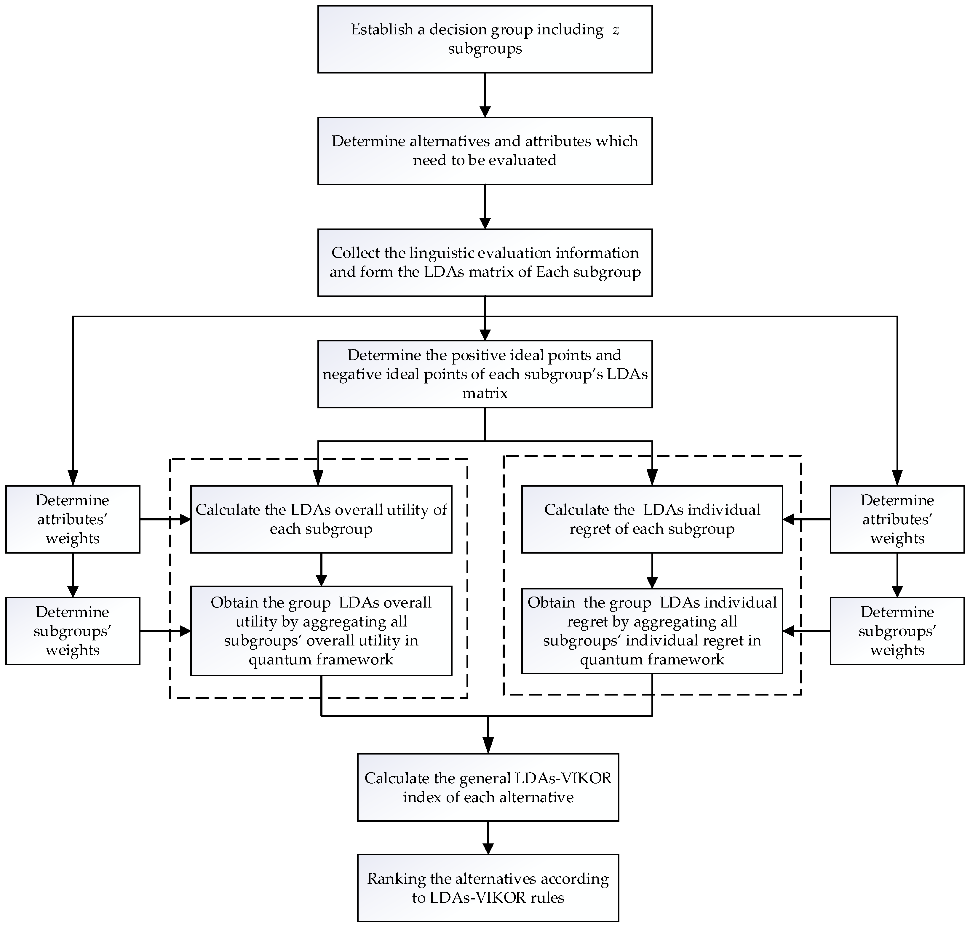
An LDAs-MAGDM problem includes $m$ alternatives $x_i \left(i=1,\dots ,m\right)$ and $n$ attributes $c_j\left(j=1,\dots ,n\right)$, and a decision group consists of several subgroups. Here, a subgroup can be viewed as a decision-maker as mentioned in Section 3, and an LAD of a subgroup is the “group evaluation” mentioned in Section 2.1. For simplicity, the $k$-th subgroup is represented by $d_k\left(k=1,\dots ,z\right)$. ${\omega }_j=\left({\omega }_1,\dots ,{\omega }_n\right)$, and $\lambda =\left({\lambda }_1,\dots ,{\lambda }_z\right)$ are the subjective weights of attributes and subgroups, respectively. Team members in each subgroup can express their opinions by the pre-given LTs with freedom. Then, the linguistic evaluation given by team members of each subgroup is collected and summarized into LDA; the $k$-th subgroup’s LDAs preference matrix is listed as:

$$X^k={\left(x_{ij}\right)}^k=\left(\begin{array}{ccc}{x}_{11}^k& \cdots & x_{1n}^k\\ ⋮& \ddots & ⋮\\ x_{m1}^k& \cdots & x_{mn}^k\end{array}\right)$$

where $x_{ij}^k$ is an LDA of alternative $x_i$ towards attribute $c_j$ provided by subgroup $d_k$. The method proposed in this paper dealing with MAGDM problem mainly consists of nine steps, and the graphic process is shown in Figure 6.

Figure 6. The process of quantum-based LDAs–VIKOR MAGDM model.

• Establish a decision group including $z$ subgroups $d_1,d_2,\dots ,d_z$, and determine alternatives and attributes;
• Collect the linguistic evaluation information of each subgroup and form the LDAs matrix of subgroup $d_k$;
• Determine the weights of attributes and subgroups;
• Determine the positive ideal points and negative ideal points in each column of each subgroup’s LDAs matrix;
• Calculate the LDAs overall utility and LDAs individual regret of $d_k$ according to positive ideal points and negative ideal points;
• Integrate all subgroups’ LDAs overall utility and LDAs individual regret in the quantum decision framework considering the asymmetric interference effects, respectively;
• Obtain the group LDAs overall utility and LDAs individual regret;
• Calculate the general LDAs–VIKOR index of each alternative;
• Rank the alternative according to the ranking rules of LDAs–VIKOR.

4.2. The Quantum LDAs–VIKOR Decision Model for MAGDM

Compared with the traditional MAGDM framework based on VIKOR, the critical parts of the method proposed in this paper are steps 5, 6, 7, and 8. These steps are crucial for an LDAs–VIKOR method, building a quantum framework that considers asymmetric interference effects.

4.2.1. The LDAs–VIKOR Method

To solve MAGDM problem with conflicting attributes, our study proposes an LADs-VIKOR method. Opricovic [23] developed VIKOR method according to $L_p$-metric:

$$L_{p,j}={\left\{{{\displaystyle \sum }}_{j=1}^n{\left[{\omega }_j\left(T_j^{*}-T_{ij}\right)/\left(T_j^{*}-T_j^{-}\right)\right]}^p\right\}}^{1/p},1\le p\le \infty ;i=1,\dots ,m$$

where ${\omega }_j=\left({\omega }_1,\dots ,{\omega }_n\right)$ is the weight of attributes as before and $T_j^{*}$ and $T_j^{-}$ are the positive ideal point and negative ideal point, respectively, of the $j$-th column of the attribute. Then, the overall utility and individual regret is defined in the form of LDAs as:

Definition 4.

The LDAs overall utility measure ($LDAS$) over alternative$x_i$can be calculated by:

$$LDA{S}_i={{\displaystyle \sum }}_{j=1}^n\left[{\omega }_{j}d\left(T_j^{*},T_{ij}\right)/d\left(T_j^{*},T_j^{-}\right)\right]$$

(12)

Definition 5.

The LDAs individual regret measure ($LDAR$) over alternative$x_i$can be calculated by:

$$LDA{R}_i=ma{x}_j\left[{\omega }_{j}d\left(T_j^{*},T_{ij}\right)/d\left(T_j^{*},T_j^{-}\right)\right]$$

(13)

The general LDAs–VIKOR index $LDA{Q}_i$ of alternative $x_i$ is:

$$LDA{Q}_i=\gamma \frac{\left(LDA{S}_i-LDA{S}^{*}\right)}{\left(LDA{S}^{-}-LDA{S}^{*}\right)}+\left(1-\gamma \right)\frac{\left(LDA{R}_i-LDA{R}^{*}\right)}{\left( LDA{R}^{-}-LDA{R}^{*}\right)}$$

(14)

where $LDA{S}^{*}=minLDA{S}_i$, $LDA{S}^{-}=maxLDA{S}_i$, $LDA{R}^{*}=minLDA{R}_i$, $LDA{R}^{-}=maxLDA{R}_i$, and $\gamma \in \left[0,1\right]$ represents the weight of the overall utility. If $\gamma >0.5$, it means that the decision-maker tends to choose the maximum overall utility strategy; if $\gamma <0.5$, the decision-maker tends to choose the minimum individual regret strategy and reaches a consensus if $v=0.5$.

Based on the value of $LDA{Q}_i$ and the following two conditions, we can rank the alternatives.

Con₁: Acceptable advantage. $LDA{Q}_m-LDA{Q}_1\ge 1/\left(m-1\right)$, if $m=2$, then the first and second position in the rank list of $LDA{Q}_i$ are the alternative $x_1$ and $x_2$, respectively;

Con₂: Acceptable stability. $x_1$ should also be the best in the rank list of $LDA{S}_i$ or $LDA{R}_i$.

• If both Con₁ and Con₂ are satisfied, then $x_1$ is the best solution.
• If Con₁ is not satisfied, then $\left\{x_1,\dots ,x_m\right\}$ is a set of compromise solutions whenever the maximum value of $m$ satisfy the formula: $LDA{Q}_m-LDA{Q}_1<1/\left(m-1\right)$.
• If Con₂ is not satisfied, then the compromise solutions are alternatives $x_1$ and $x_2$.

The determination of distance $d\left(T_j^{*},T_{ij}\right)$ and $d\left(T_j^{*},T_j^{-}\right)$ is the key to calculate $LDA{S}_i$ and $LDA{R}_i$. The previous studies of distance measurements for measuring LDAs have some limitations; for example, the use of the max and min operator would lead to loss of information [14]. To address this issue, a new distance measurement for LDAs with sample capacity is defined as follows.

Definition 6.

Let $T_1=\{\left(l_v^1,p_v^1\right)|l_v^1\in L,p_v^1\in \left[0, 1\right],{\displaystyle \sum }_v{p}_v^1=1,size=N\}$and $T_2=\{\left(l_v^2,p_v^2\right)|l_v^2\in L,p_v^2\in \left[0, 1\right],{\displaystyle \sum }_v{p}_v^2=1,size=N\}$be any two LDAs. The generalized distance measure between $T_1$and $T_2$can then be defined as follows:

$$d\left(T_1,T_2\right)=\frac{1}{g+1}{{\displaystyle \sum }}_{v=0}^g\{{[f\left(l_v^1\right)p_v^1]}^{\propto }-{\left[f\left(l_v^2\right)p_v^2\right]}^{\propto }]{\}}^{\frac{1}{\propto }}$$

(15)

where $g+1$is the total number of $L$, $v=\left(0,1,2,\dots g\right)$, and $f$is the linguistic scale function as before.

Evidently, with the different value of$\propto$, it represents different distance expressions.

(1)

When$\propto =1$, it is the Hamming-Hausdorff distance;

(2)

When$\propto =2$, it is the Euclidean-Hausdorff distance.

Theorem 1.

Let$T_1=\{\left(l_v^1,p_v^1\right)|l_v^1\in L,p_v^1\in \left[0, 1\right],{\displaystyle \sum }_v{p}_v^1=1,size=N\}$, $T_2=\{\left(l_v^2,p_v^2\right)|l_v^2\in L,p_v^2\in \left[0, 1\right],{\displaystyle \sum }_v{p}_v^2=1,size=N\}$and$T_3=\{\left(l_v^3,p_v^3\right)|l_v^3\in L,p_v^3\in \left[0, 1\right],{\displaystyle \sum }_v{p}_v^3=1,size=N\}$be any three LDAs. Then, Equation (15) satisfied the following properties:

(1)

Non-negativity:$d\left(T_1,T_2\right)\ge 0$;

(2)

Reflexivity:$d\left(T_1,T_1\right)=0$;

(3)

Reciprocity:$d\left(T_1,T_2\right)=d\left(T_2,T_1\right)$;

(4)

Transitivity: if$d\left(T_1,T_2\right)=0$,$d\left(T_2,T_3\right)=0$, then$d\left(T_1,T_3\right)=0$.

Properties (1)–(3) are easily proved, and their proofs are omitted. We give the proof of property (4) as follows:

Proof. 

According to Definition 6, if $d\left(T_1,T_2\right)=0$, $d\left(T_2,T_3\right)=0$, then, $T_1~T_2$ and $T_2~T_3$, we can deduce that $T_1~T_3$, then $d\left(T_1,T_3\right)=0$. □

4.2.2. Form Opinion of Subgroup $d_k$ by LDAs–VIKOR Method

First, we collect LDAs information to form LDAs decision matrix of each subgroup. Then we can use Equation (1) to compare LDAs in each column of the formed matrix to determine the positive ideal LDAs $T_j^{*k}$ and the negative ideal LDAs $T_j^{-k}$ of the $j$-th column. Here, we adopt the linguistic scale function in [14]: $f\left(l{t}_v\right)=f\left(l{t}_{\vartheta \left(t\right)}\right)=\vartheta \left(x\right)=x/2t^{\prime },x=\left\{0,1,\dots ,2t^{\prime }\right\}$. Second, let $T_j^{*k}=ma{x}_j{T}_{ij}^k, T_j^{-k}=mi{n}_j{T}_{ij}^k$, if the $j$-th column represents a benefit (if represents a cost then reverse). Then, we use the newly proposed LDAs distance measurement in Section 4.2.1 to calculate the $LDA{S}_i^k$ and $LDA{R}_i^k$.

(1)

The LDAs overall utility over alternative $x_i$ of subgroup $d_k$ could be calculated as follows:

$$LDA{S}_i^k={{\displaystyle \sum }}_{j=1}^n\left[{\omega }_j^{k}d\left(T_j^{*k},T_{ij}^k\right)/d\left(T_j^{*k},T_j^{-k}\right)\right]$$

(16)

(2)

The LDAs individual regret over alternative $x_i$ of subgroup $d_k$ could be calculated as follows:

$$LDA{R}_i^k=max\left[{\omega }_j^{k}d\left(T_j^{*k},T_{ij}^k\right)/d\left(T_j^{*k},T_j^{-k}\right)\right]$$

(17)

where ${\omega }_j^k$ is the weight of attribute $c_j$ of subgroup $d_k$. $d\left(T_j^{*k},T_{ij}^k\right)$ and $d\left(T_j^{*k},T_j^{-k}\right)$ represent the distance to ‘‘ideal’’ solution of each alternative. It can be computed by Equation (15).

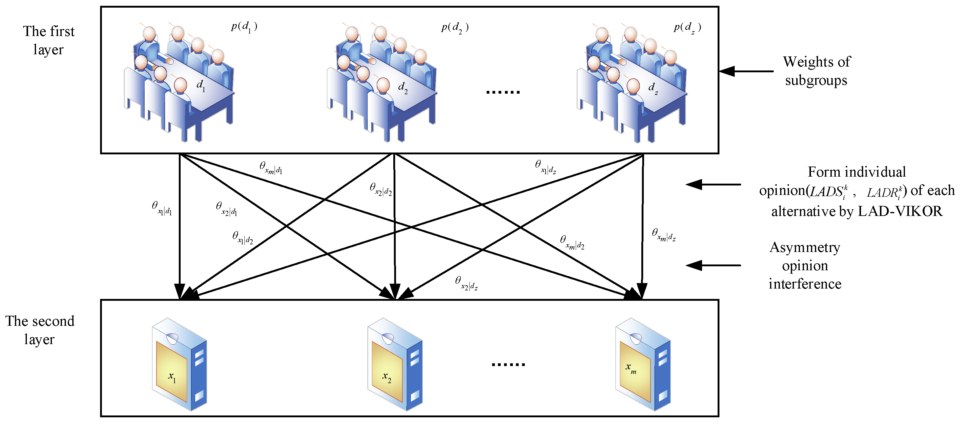
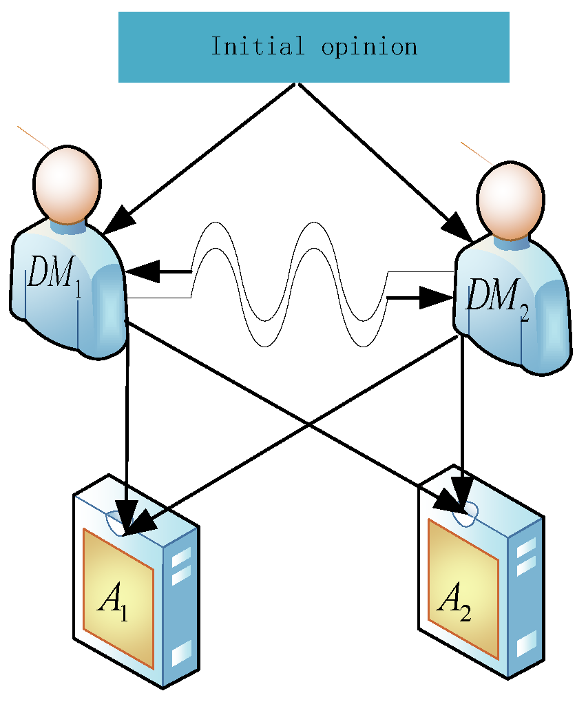
4.2.3. Aggregate Opinions of All Subgroups in Quantum Decision Framework

After deriving the evaluation result ($LDA{S}_i^k$ and $LDA{R}_i^k$) of each subgroup based on the LDAs–VIKOR method, we need to integrate the evaluation results of all subgroups by an effective information integration technology to derive the group’s $LDA{S}_i$ and $LDA{R}_i$ to compute the final closeness coefficient $LDA{Q}_i$ to the ideal solution of each alternative. Now, let us explore the asymmetric opinions interference among subgroups in a quantum-based aggregation mode first.

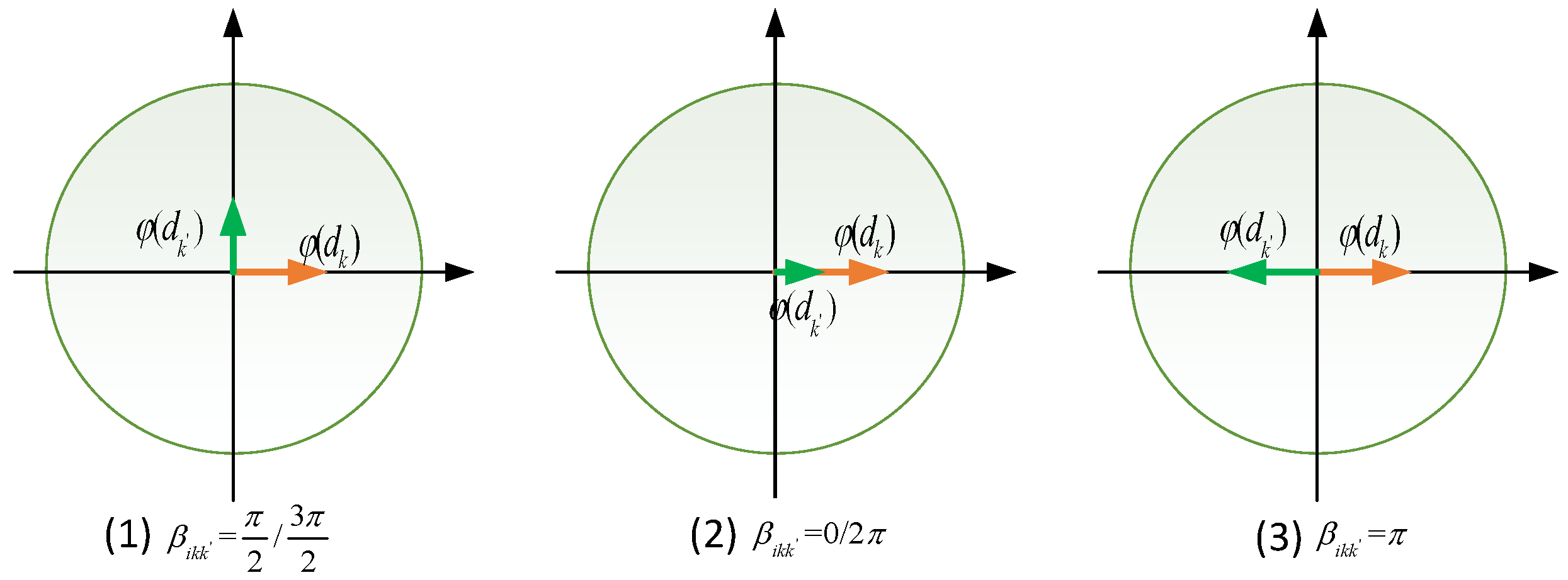
• Asymmetric opinion interference among any two subgroups in a quantum decision framework.

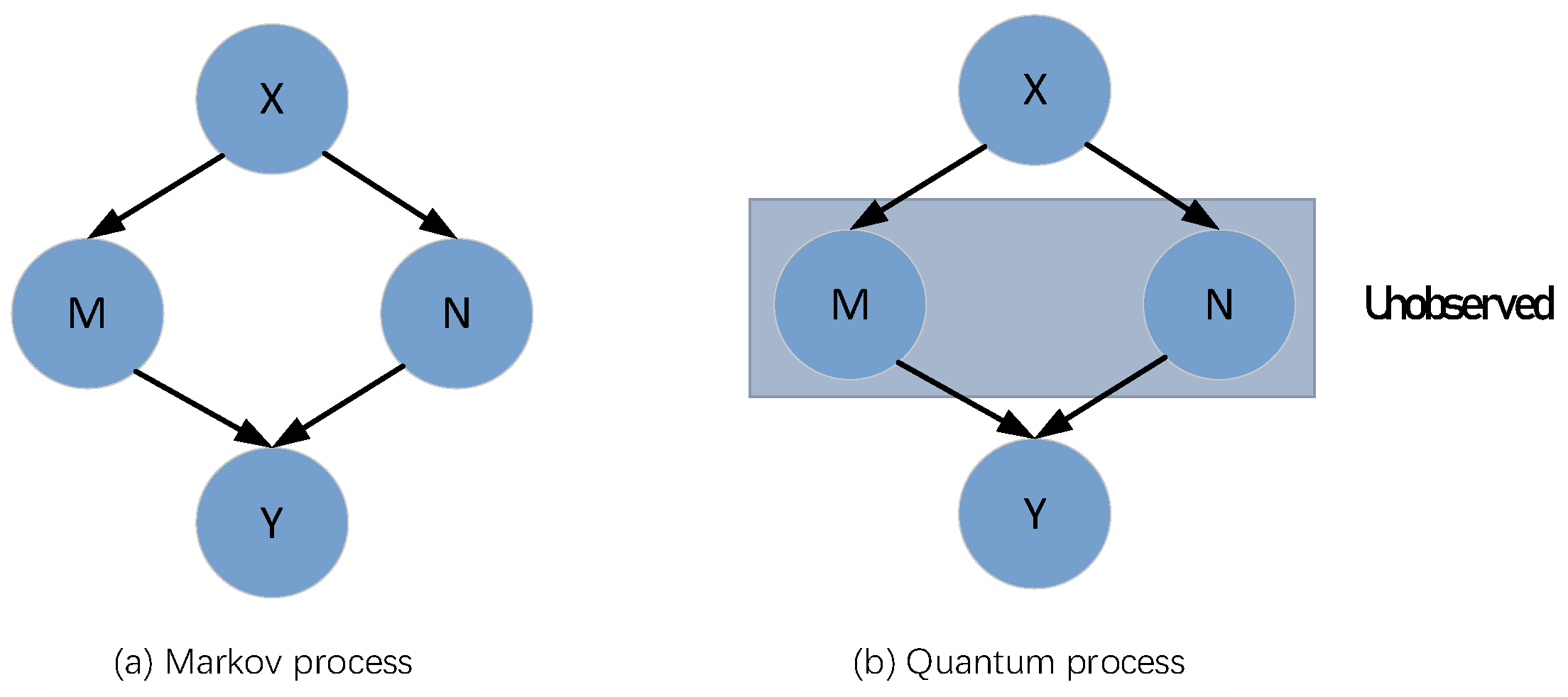
The classical total probability law can be written as Equation (18). It is also depicted as the classical “Bayes network” (BN).

$$P\left(x_i\right)={{\displaystyle \sum }}_{k=1}^{z}P\left(d_k\right)P\left(x_i|d_k\right),i=1,2\dots ,m, k=1,2,\dots ,z$$

(18)

where ${{\displaystyle \sum }}_{k=1}^{z}P\left(d_k\right)=1$. In this way, we can derive $LDA{S}_i$ and $LDA{R}_i$ of $x_i$ in the form of probability, respectively,

$${LDA{S}_i}^{\prime }={{\displaystyle \sum }}_{k=1}^{z}P\left(d_k\right)P\left(LDA{S}_i|d_k\right)$$

(19)

$${LDA{R}_i}^{\prime }={{\displaystyle \sum }}_{k=1}^{z}P\left(d_k\right)P\left(LDA{R}_i|d_k\right)$$

(20)

where $P\left(LDA{S}_i|d_k\right)$ = $LDA{S}_i^k$/${\displaystyle \sum }_{i=1}^{m}LDA{S}_i^k$, $P\left(LDA{R}_i|d_k\right)$ = $LDA{R}_i^k$/${\displaystyle \sum }_{i=1}^{m}LDA{R}_i^k$. $P\left(d_k\right)$ is the weight of subgroup $d_k$.

In QPT, the subjective belief state is a superposition of several specific states. In this situation, one can extend the classical BN to a quantum-based BN (see Figure 7) based on [29]. The belief state in the first layer can be written by $|D⟩$, and the decision state in the second layer by $|X⟩$, respectively.

$$|D⟩={{\displaystyle \sum }}_{k=1}^z\phi \left(d_k\right)|d_k⟩$$

(21)

$$|X⟩={{\displaystyle \sum }}_{i=1}^m\phi \left(x_i\right)|x_i⟩$$

(22)

Figure 7. A quantum-based BN of a MAGCD problem.

For example, we assume that there is a belief state $|d_1⟩$ in Hilbert space, then the corresponding amplitude probability is $\phi \left(d_1\right)$. An intermediate state can be represented by $|X|D⟩$, which joints the belief state and decision state. The state $|X|D⟩$ can be written as:

$$|X|D⟩={{\displaystyle \sum }}_{k=1}^z{{\displaystyle \sum }}_{i=1}^m\phi \left(x_i|d_k\right)|x_i|d_k⟩$$

(23)

State $|X⟩$ can be determined through $z\times m$ possible paths:

$$|X⟩=|D⟩\times |X|D⟩={{\displaystyle \sum }}_{k=1}^z{{\displaystyle \sum }}_{i=1}^m\phi \left(d_k\right)\phi \left(x_i|d_k\right)|x_i⟩|x_i|d_k⟩$$

(24)

During the process of decision-making, subgroups’ opinions are often integrated simultaneously by the final decision-maker (director) instead of one-by-one. Therefore, the paths are naturally indistinguishable, and the decision state’s probability can be represented by the square of the summation of the amplitude probabilities of all possible paths. The probability of $x_i$ can be easily obtained by Equation (25) according to the total probability quantum interference law [50]:

$$P\left(x_i\right)={\left|{{\displaystyle \sum }}_{k=1}^z{e}^{{\theta }_{d_k}}\psi \left(d_k\right)e^{{\theta }_{x_i|d_k}}\psi \left(x_i|d_k\right)\right|}^2$$

(25)

He et al. [29] let the phase angles belonging to any possible paths that point to the identical alternative to be the same, i.e., ${\theta }_{x_i|d_1}={\theta }_{x_i|d_2}=\dots ={\theta }_{x_i|d_z}$, then the interference term is $cos\left({\theta }_k-{\theta }_{k^{\prime }}\right)$. However, as mentioned in Section 3, ${\theta }_{x_i|d_1}={\theta }_{x_i|d_2}=\dots ={\theta }_{x_i|d_z}$ is just a special case, i.e., the symmetric interference effects. The more common situation is the asymmetric interference. i.e., ${\theta }_{x_i|d_1}\ne {\theta }_{x_i|d_2}\ne \dots \ne {\theta }_{x_i|d_z}$, or some are equal and some are not equal, then the expansion of Equation (25) can be written as:

$$\begin{array}{ll}P\left(x_i\right)=& [{\displaystyle \sum }_{k=1}^{z}P\left(d_k\right)P\left(x_i|d_k\right)+\\ & 2{\displaystyle \sum }_{k=1}^{z-1}{\displaystyle \sum }_{k^{\prime }=k+1}^z\sqrt{P\left(d_k\right)}\sqrt{P\left(x_i|d_k\right)}\\ & \sqrt{P\left(d_{k^{\prime }}\right)}\sqrt{P\left(x_i|d_{k^{\prime }}\right)}\cos \left({\theta }_{ik}-{\theta }_{i{k}^{\prime }}\right)]/\eta \end{array}$$

(26)

$\eta$ is a normalization operator, $\eta ={\displaystyle \sum }_{i=1}^m{\left|{\displaystyle \sum }_{k=1}^z{e}^{{\theta }_{d_k}}\psi \left(d_k\right)e^{{\theta }_{x_i|d_k}}\psi \left(x_i|d_k\right)\right|}^2$.

Now, the $LDA{S}_i$ and $LDA{R}_i$ of $x_i$ can be rewritten as:

$$\begin{array}{ll}LDA{S}_i& =\&[LDA{S}_i^{\prime }+2{\displaystyle \sum }_{k=1}^{z-1}{\displaystyle \sum }_{k^{\prime }=k+1}^z\sqrt{P\left(d_k\right)}\sqrt{P\left(LDA{S}_i|d_k\right)}\\ & \sqrt{P\left(d_{k^{\prime }}\right)}\sqrt{P\left(LDA{S}_i|d_{k^{\prime }}\right)}\cos \left({\theta }_{ik}-{\theta }_{i{k}^{\prime }}\right)]/{\eta }_1\end{array}$$

(27)

$$\begin{array}{ll}LDA{R}_i=& [LDA{R}_i^{\prime }+2{\displaystyle \sum }_{k=1}^{z-1}{\displaystyle \sum }_{k^{\prime }=k+1}^z\sqrt{P\left(d_k\right)}\sqrt{P\left(LDA{R}_i|d_k\right)}\\ & \sqrt{P\left(d_{k^{\prime }}\right)}\sqrt{P\left(LDA{R}_i|d_{k^{\prime }}\right)}\cos \left({\theta }_{ik}-{\theta }_{i{k}^{\prime }}\right)]/{\eta }_2\end{array}$$

(28)

where $k \mathrm{and} k^{\prime }$ represents different subgroup that interact with each other. Let ${\beta }_{ik{k}^{\prime }}={\theta }_{ik}-{\theta }_{i{k}^{\prime }}, {\beta }_{ik{k}^{\prime }}\in \left[0,2\pi \right]$, which can be regarded as the subjective psychological feeling of the director towards subgroups’ different opinions; it can also can be interpreted as the director’s subjective beliefs. Three typical ${\beta }_{ik{k}^{\prime }}$ values are shown in Figure 8, corresponding to:

Figure 8. Different phases of the two subgroups of alternative $x_i$.

• When ${\beta }_{ik{k}^{\prime }}=\pi /2$, and ${\beta }_{ik{k}^{\prime }}=3\pi /2$, there is no interference among subgroups. Each subgroup is considered completely independent to others. Then the proposed model degenerates into the classical Bayesian network.
• When ${\beta }_{ik{k}^{\prime }}\in \left[0,\pi /2\right)$ and $(3\pi /2, 2\pi ]$, there exists positive interference among two subgroups. If ${\beta }_{ik{k}^{\prime }}=0$ and $2\pi$, their opinions are completely affected positively. The subgroups are regarded as complete positive-related.
• When ${\beta }_{ik{k}^{\prime }}\in \left(\pi /2,3\pi /2\right)$, there exists negative interference among two subgroups, if ${\beta }_{ik{k}^{\prime }}=\pi$, their opinions are completely affected negatively. The subgroups are regarded as complete negative-related.

2.

Determine the value of the interference terms by belief entropy.

From Equation (26), one can find that the parameters’ (${\beta }_{ik{k}^{\prime }}$) number will expand massively as the number of subgroups increases. The determination of ${\beta }_{ik{k}^{\prime }}$ is very important for using quantum probability theory, but there is no authoritative method yet. One method of determining the interference terms is similarity heuristic [53]; the other is based on belief entropy [54,55]. Since the similarity heuristic is highly subjective, we choose to adopt belief entropy to determine the value of asymmetric interference terms. The expression of belief entropy is defined by [56]:

$$D_b=-E_b={{\displaystyle \sum }}_{L\subseteq X}{M}_{L}lo{g}_2{M}_L/\left(2^{\left|L\right|}-1\right)$$

(29)

where $X$ is the set of options or events, $L$ is a subset of $X$, the evidence’s support degree on $X$ is represented by mass function $M_L$, $\left|L\right|$ is the cardinality of $L$, which represents the number of the final choices or answers to a query. In our MAGDM problem, $\left|L\right|$ either represents the subgroups’ number in the first layer or the choice under each subgroup in the second layer. The key of obtaining the belief entropy is to determine $M_L$. Here, we substitute belief distance [54] to $M_L$. The similarities of two of the decision vectors can be measured by belief distance. The belief distance is closely related to the connection vector [55], which is denoted by the combination of any two subgroups with respect to the same alternative. One can write it as: $\stackrel{\rightharpoonup }{\xi }=\left[\begin{array}{c}{\mu }_{iq}\\ {\vartheta }_{iq}\end{array}\right]$, $i=1,\dots ,m, q=1,\dots ,z\left(z-1\right)/2$. The function of belief distance is defined as follows:

$$B_{iq}=\left|{\mu }_{iq}+\left(\left|{\mu }_{iq}-\delta \right|-\left|{\vartheta }_{iq}-\delta \right|\right)/\left(\left|{\mu }_{iq}-\delta \right|+\left|{\vartheta }_{iq}-\delta \right|\right)\right|$$

(30)

If $\left|{\mu }_{iq}-\delta \right|\le \left|{\vartheta }_{iq}-\delta \right|$, then we should switch the position of ${\mu }_{iq}$ and ${\vartheta }_{iq}$. $\delta =1/z$ represents the average probability of each subgroup. The deviation degree of ${\mu }_{iq}$ and ${\vartheta }_{iq}$ from the average probability is represented by $\left|{\mu }_{iq}-\delta \right|$ and $\left|{\vartheta }_{iq}-\delta \right|$, and $M_L$ in Equation (29) can be substituted with $B_{iq}$. The belief entropy can be modified as:

$$D_{iq}=B_{iq}lo{g}_2{B}_{iq}/\left(2^L-1\right)$$

(31)

It is easy to find that the Equation (31) has some differences compared with Equation (29). The summation of the Equation (31) is canceled, and $L$ is fixed to 2. The reason for these modifications is because this paper considers the interaction between any two subgroups instead of the whole group. We can use Equation (32) to normalize ${D^{\prime }}_{iq}$ to ensure that ${D^{\prime }}_{iq}$ is in $\left[-1,1\right]$:

$${D^{\prime }}_{iq}=2\left[\left(D_{iq}-min{D}_b\right)/\left(max{D}_b-min{D}_b\right)\right]-1$$

(32)

where $max{D}_b=0$, $min{D}_b=\left(2-\delta \right)/lo{g}_2\left(2-\delta \right)/\left(2^{z\left(z-1\right)/2}-1\right)$. For the detailed derivation process of the $max{D}_b$ and $min{D}_b$, please refer to [55].

According to [54], $cos{\beta }_{ik{k}^{\prime }}$ can be replaced by ${D^{\prime }}_{iq}$, i.e., ${D^{\prime }}_{iq}=cos{\beta }_{ik{k}^{\prime }}$, and we can calculate the exact value of $LDA{S}_i$, $LDA{R}_i$. The value of the general LDAs–VIKOR index $LDA{Q}_i$ can also be computed by Equation (14).

5. Case Study

In this section, we apply the proposed model to evaluate internet finance service (IFS), which is adopted from [57]. An enterprise hopes to select an internet financial platform to promote capital flow and ensure its security. After preliminary screening, four alternative platforms need to be finally evaluated; $A_1$: Alipay, $A_2$: YeePay, $A_3$: JD Finance, $A_4$: ShengPay. The internet finance platform evaluation includes five attributes; $c_1$: Cultural Environment, $c_2$: Technical Innovation, $c_3$: Policy Support, $c_4$: Industrial Competitiveness, $c{r}_5$: International Influence. The director forms three subgroups $d_1, d_2, d_3$ to participate in the evaluation problem, their weighting vector $\lambda =\left\{0.4,0.3,0.3\right\}$ is pre-given, and the weights of five attributes are also pre-given by subgroups, respectively (see Table 1, Table 2 and Table 3). A set of LTs are given as: $LTs=\left\{l{t}_0:very bad, l{t}_1:bad,l{t}_2:moderate,l{t}_3: good,l{t}_4:very good\right\}$. Each team member in a subgroup can choose an element in the set of LTs to evaluate alternatives to form LDAs. For example, let 16 team members give evaluation to the $c_j$ of $A_i$, where 8 of them think it is $very good$, 6 of them think it is $good$, 2 of them think it is $moderate$, and none of them think it is $bad$ or $very bad$. Then, the LDA can be written as: $\left\{\left(l{t}_0,0/16\right),\left(l{t}_1,0/16\right),\left(l{t}_2,2/16\right),\left(l{t}_3,6/16\right),\left(l{t}_4,8/16\right)|N=16\right\}$. The number $0/16$ represents the probability distribution of $l{t}_0$ when the sample capacity is 16.

Table 1. LDAs decision matrix of $d_1$.

	${\mathit{c}}_1 \left(0.2\right)$	${\mathit{c}}_2 \left(0.3\right)$	${\mathit{c}}_3 \left(0.1\right)$	${\mathit{c}}_4 \left(0.2\right)$	${\mathit{c}}_5 \left(0.2\right)$
$A_1$	$\left\{\begin{array}{c}\left(l{t}_0,0/16\right),\left(l{t}_1,0/16\right),\\ \left(l{t}_2,0/16\right),\left(l{t}_3,8/16\right),\\ \left(l{t}_4,8/16\right)|N_{11}^1=16\end{array}\right\}$	$\left\{\begin{array}{c}\left(l{t}_0,0/20\right),\left(l{t}_1,0/20\right),\\ \left(l{t}_2,0/20\right),\left(l{t}_3,10/20\right),\\ \left(l{t}_4,10/20\right)|N_{12}^1=20\end{array}\right\}$	$\left\{\begin{array}{c}\left(l{t}_0,0/16\right),\left(l{t}_1,0/16\right),\\ \left(l{t}_2,4/16\right),\left(l{t}_3,4/16\right),\\ \left(l{t}_4,8/16\right)|N_{13}^1=16\end{array}\right\}$	$\left\{\begin{array}{c}\left(l{t}_0,0/20\right),\left(l{t}_1,0/20\right),\\ \left(l{t}_2,2/20\right),\left(l{t}_3,4/20\right),\\ \left(l{t}_4,14/20\right)|N_{14}^1=20\end{array}\right\}$	$\left\{\begin{array}{c}\left(l{t}_0,0/20\right),\left(l{t}_1,0/20\right),\\ \left(l{t}_2,2/20\right),\left(l{t}_3,6/20\right),\\ \left(l{t}_4,12/20\right)|N_{15}^1=20\end{array}\right\}$
$A_2$	$\left\{\begin{array}{c}\left(l{t}_0,0/16\right),\left(l{t}_1,0/16\right),\\ \left(l{t}_2,,2/16\right),\left(l{t}_3,8/16\right),\\ \left(l{t}_4,6/16\right)|N_{21}^1=16\end{array}\right\}$	$\left\{\begin{array}{c}\left(l{t}_0,0/20\right),\left(l{t}_1,0/20\right),\\ \left(l{t}_2,6/20\right),\left(l{t}_3,10/20\right),\\ \left(l{t}_4,4/20\right)|N_{22}^1=20\end{array}\right\}$	$\left\{\begin{array}{c}\left(l{t}_0,0/16\right),\left(l{t}_1,0/16\right),\\ \left(l{t}_2,4/16\right),\left(l{t}_3,6/16\right),\\ \left(l{t}_4,6/16\right)|N_{23}^1=16\end{array}\right\}$	$\left\{\begin{array}{c}\left(l{t}_0,0/20\right),\left(l{t}_1,0/20\right),\\ \left(l{t}_2,7/20\right),\left(l{t}_3,9/20\right),\\ \left(l{t}_4,4/20\right)|N_{24}^1=20\end{array}\right\}$	$\left\{\begin{array}{c}\left(l{t}_0,0/20\right),\left(l{t}_1,0/20\right),\\ \left(l{t}_2,6/20\right),\left(l{t}_3,8/20\right),\\ \left(l{t}_4,6/20\right)|N_{25}^1=20\end{array}\right\}$
$A_3$	$\left\{\begin{array}{c}\left(l{t}_0,0/16\right),\left(l{t}_1,0/16\right),\\ \left(l{t}_2,,0/16\right),\left(l{t}_3,6/16\right),\\ \left(l_4,10/16\right)|N_{31}^1=16\end{array}\right\}$	$\left\{\begin{array}{c}\left(l{t}_0,0/20\right),\left(l{t}_1,0/20\right),\\ \left(l{t}_2,,0/20\right),\left(l{t}_3,6/20\right),\\ \left(l{t}_4,14/20\right)|N_{32}^1=20\end{array}\right\}$	$\left\{\begin{array}{c}\left(l{t}_0,0/16\right),\left(l{t}_1,0/16\right),\\ \left(l{t}_2,4/16\right),\left(l{t}_3,2/16\right),\\ \left(l{t}_4,10/16\right)|N_{33}^1=16\end{array}\right\}$	$\left\{\begin{array}{c}\left(l{t}_0,0/20\right),\left(l{t}_1,0/20\right),\\ \left(l{t}_2,2/20\right),\left(l{t}_3,6/20\right),\\ \left(l{t}_4,12/20\right)|N_{34}^1=20\end{array}\right\}$	$\left\{\begin{array}{c}\left(l{t}_0,0/20\right),\left(l{t}_1,0/20\right),\\ \left(l{t}_2,4/20\right),\left(l{t}_3,4/20\right),\\ \left(l{t}_4,12/20\right)|N_{35}^1=20\end{array}\right\}$
$A_4$	$\left\{\begin{array}{c}\left(l{t}_0,0/16\right),\left(l{t}_1,0/16\right),\\ \left(l{t}_2,,6/16\right),\left(l{t}_3,6/16\right),\\ \left(l{t}_4,4/16\right)|N_{41}^1=16\end{array}\right\}$	$\left\{\begin{array}{c}\left(l{t}_0,0/20\right),\left(l{t}_1,0/20\right),\\ \left(l{t}_2,,6/20\right),\left(l{t}_3,8/20\right),\\ \left(l{t}_4,6/20\right)|N_{42}^1=20\end{array}\right\}$	$\left\{\begin{array}{c}\left(l{t}_0,0/16\right),\left(l{t}_1,0/16\right),\\ \left(l{t}_2,6/16\right),\left(l{t}_3,6/16\right),\\ \left(l{t}_4,4/16\right)|N_{43}^1=16\end{array}\right\}$	$\left\{\begin{array}{c}\left(l{t}_0,0/20\right),\left(l{t}_1,0/20\right),\\ \left(l{t}_2,3/20\right),\left(l{t}_3,9/20\right),\\ \left(l{t}_4,8/20\right)|N_{44}^1=20\end{array}\right\}$	$\left\{\begin{array}{c}\left(l{t}_0,0/20\right),\left(l{t}_1,0/20\right),\\ \left(l{t}_2,6/20\right),\left(l{t}_3,10/20\right),\\ \left(l{t}_4,4/20\right)|N_{45}^1=20\end{array}\right\}$

Table 2. LDAs decision matrix of $d_2$.

	${\mathit{c}}_1 \left(0.2\right)$	${\mathit{c}}_2 \left(0.2\right)$	${\mathit{c}}_3 \left(0.3\right)$	${\mathit{c}}_4 \left(0.1\right)$	${\mathit{c}}_5 \left(0.2\right)$
$A_1$	$\left\{\begin{array}{c}\left(l{t}_0,0/10\right),\left(l{t}_1,0/10\right),\\ \left(l{t}_2,0/10\right),\left(l{t}_3,4/10\right),\\ \left(l{t}_4,6/10\right)|N_{11}^2=10\end{array}\right\}$	$\left\{\begin{array}{c}\left(l{t}_0,0/15\right),\left(l{t}_1,0/15\right),\\ \left(l{t}_2,0/15\right),\left(l{t}_3,6/15\right),\\ \left(l{t}_4,9/15\right)|N_{12}^2=15\end{array}\right\}$	$\left\{\begin{array}{c}\left(l{t}_0,0/15\right),\left(l{t}_1,0/15\right),\\ \left(l{t}_2,2/15\right),\left(l{t}_3,4/15\right),\\ \left(l{t}_4,9/15\right)|N_{13}^2=15\end{array}\right\}$	$\left\{\begin{array}{c}\left(l{t}_0,0/15\right),\left(l{t}_1,0/15\right),\\ \left(l{t}_2,3/15\right),\left(l{t}_3,6/15\right),\\ \left(l{t}_4,6/15\right)|N_{14}^2=15\end{array}\right\}$	$\left\{\begin{array}{c}\left(l{t}_0,0/15\right),\left(l{t}_1,0/15\right),\\ \left(l{t}_2,2/15\right),\left(l{t}_3,3/15\right),\\ \left(l{t}_4,10/15\right)|N_{15}^2=15\end{array}\right\}$
$A_2$	$\left\{\begin{array}{c}\left(l{t}_0,0/10\right),\left(l{t}_1,0/10\right),\\ \left(l{t}_2,0/10\right),\left(l{t}_3,6/10\right),\\ \left(l{t}_4,4/10\right)|N_{21}^2=10\end{array}\right\}$	$\left\{\begin{array}{c}\left(l{t}_0,0/15\right),\left(l{t}_1,0/15\right),\\ \left(l{t}_2,3/15\right),\left(l{t}_3,6/15\right),\\ \left(l{t}_4,6/15\right)|N_{22}^2=15\end{array}\right\}$	$\left\{\begin{array}{c}\left(l{t}_0,0/15\right),\left(l{t}_1,0/15\right),\\ \left(l{t}_2,3/15\right),\left(l{t}_3,3/15\right),\\ \left(l{t}_4,9/15\right)|N_{23}^2=15\end{array}\right\}$	$\left\{\begin{array}{c}\left(l{t}_0,0/15\right),\left(l{t}_1,0/15\right),\\ \left(l{t}_2,3/15\right),\left(l{t}_3,4/15\right),\\ \left(l{t}_4,8/15\right)|N_{24}^2=15\end{array}\right\}$	$\left\{\begin{array}{c}\left(l{t}_0,0/15\right),\left(l{t}_1,0/15\right),\\ \left(l{t}_2,4/15\right),\left(l{t}_3,3/15\right),\\ \left(l{t}_4,8/15\right)|N_{25}^2=15\end{array}\right\}$
$A_3$	$\left\{\begin{array}{c}\left(l{t}_0,0/10\right),\left(l{t}_1,0/10\right),\\ \left(l{t}_2,0/10\right),\left(l{t}_3,8/10\right),\\ \left(l{t}_4,2/10\right)|N_{31}^2=10\end{array}\right\}$	$\left\{\begin{array}{c}\left(l{t}_0,0/15\right),\left(l{t}_1,0/15\right),\\ \left(l{t}_2,0/15\right),\left(l{t}_3,9/15\right),\\ \left(l{t}_4,6/15\right)|N_{32}^2=15\end{array}\right\}$	$\left\{\begin{array}{c}\left(l{t}_0,0/15\right),\left(l{t}_1,0/15\right),\\ \left(l{t}_2,1/15\right),\left(l{t}_3,2/15\right),\\ \left(l{t}_4,12/15\right)|N_{33}^2=15\end{array}\right\}$	$\left\{\begin{array}{c}\left(l{t}_0,0/15\right),\left(l{t}_1,0/15\right),\\ \left(l{t}_2,1/15\right),\left(l{t}_3,7/15\right),\\ \left(l{t}_4,7/15\right)|N_{34}^2=15\end{array}\right\}$	$\left\{\begin{array}{c}\left(l{t}_0,0/15\right),\left(l{t}_1,0/15\right),\\ \left(l{t}_2,3/15\right),\left(l{t}_3,3/15\right),\\ \left(l{t}_4,9/15\right)|N_{35}^2=15\end{array}\right\}$
$A_4$	$\left\{\begin{array}{c}\left(l{t}_0,0/10\right),\left(l{t}_1,0/10\right),\\ \left(l{t}_2,4/10\right),\left(l{t}_3,4/10\right),\\ \left(l{t}_4,2/10\right)|N_{41}^2=10\end{array}\right\}$	$\left\{\begin{array}{c}\left(l{t}_0,0/15\right),\left(l{t}_1,0/15\right),\\ \left(l{t}_2,4/15\right),\left(l{t}_3,8/15\right),\\ \left(l{t}_4,3/15\right)|N_{42}^2=15\end{array}\right\}$	$\left\{\begin{array}{c}\left(l{t}_0,0/15\right),\left(l{t}_1,0/15\right),\\ \left(l{t}_2,6/15\right),\left(l{t}_3,7/15\right),\\ \left(l{t}_4,2/15\right)|N_{43}^2=15\end{array}\right\}$	$\left\{\begin{array}{c}\left(l{t}_0,0/15\right),\left(l{t}_1,0/15\right),\\ \left(l{t}_2,2/15\right),\left(l{t}_3,8/15\right),\\ \left(l{t}_4,5/15\right)|N_{44}^2=15\end{array}\right\}$	$\left\{\begin{array}{c}\left(l{t}_0,0/15\right),\left(l{t}_1,0/15\right),\\ \left(l{t}_2,3/15\right),\left(l{t}_3,10/15\right),\\ \left(l{t}_4,2/15\right)|N_{45}^2=15\end{array}\right\}$

Table 3. LDAs decision matrix of $d_3$.

	${\mathit{c}}_1 \left(0.2\right)$	${\mathit{c}}_2 \left(0.2\right)$	${\mathit{c}}_3 \left(0.2\right)$	${\mathit{c}}_4 \left(0.2\right)$	${\mathit{c}}_5 \left(0.2\right)$
$A_1$	$\left\{\begin{array}{c}\left(l{t}_0,0/25\right),\left(l{t}_1,0/25\right),\\ \left(l{t}_2,5/25\right),\left(l{t}_3,13/25\right),\\ \left(l{t}_4,7/25\right)|N_{11}^3=25\end{array}\right\}$	$\left\{\begin{array}{c}\left(l{t}_0,0/30\right),\left(l{t}_1,0/30\right),\\ \left(l{t}_2,4/30\right),\left(l{t}_3,6/30\right),\\ \left(l{t}_4,20/30\right)|N_{12}^3=30\end{array}\right\}$	$\left\{\begin{array}{c}\left(l{t}_0,0/28\right),\left(l{t}_1,0/28\right),\\ \left(l{t}_2,8/28\right),\left(l{t}_3,10/28\right),\\ \left(l{t}_4,10/28\right)|N_{13}^3=28\end{array}\right\}$	$\left\{\begin{array}{c}\left(l{t}_0,0/30\right),\left(l{t}_1,0/30\right),\\ \left(l{t}_2,5/30\right),\left(l{t}_3,5/30\right),\\ \left(l{t}_4,20/30\right)|N_{14}^3=30\end{array}\right\}$	$\left\{\begin{array}{c}\left(l{t}_0,0/30\right),\left(l{t}_1,0/30\right),\\ \left(l{t}_2,3/30\right),\left(l{t}_3,5/30\right),\\ \left(l{t}_4,22/30\right)|N_{15}^3=30\end{array}\right\}$
$A_2$	$\left\{\begin{array}{c}\left(l{t}_0,0/25\right),\left(l{t}_1,0/25\right),\\ \left(l{t}_2,3/25\right),\left(l{t}_3,14/25\right),\\ \left(l{t}_4,8/25\right)|N_{21}^3=25\end{array}\right\}$	$\left\{\begin{array}{c}\left(l{t}_0,0/30\right),\left(l{t}_1,0/30\right),\\ \left(l{t}_2,6/30\right),\left(l{t}_3,8/30\right),\\ \left(l{t}_4,16/30\right)|N_{22}^3=30\end{array}\right\}$	$\left\{\begin{array}{c}\left(l{t}_0,0/28\right),\left(l{t}_1,0/28\right),\\ \left(l{t}_2,7/28\right),\left(l{t}_3,3/28\right),\\ \left(l{t}_4,18/28\right)|N_{23}^3=28\end{array}\right\}$	$\left\{\begin{array}{c}\left(l{t}_0,0/30\right),\left(l{t}_1,0/30\right),\\ \left(l{t}_2,6/30\right),\left(l{t}_3,18/30\right),\\ \left(l{t}_4,6/30\right)|N_{24}^3=30\end{array}\right\}$	$\left\{\begin{array}{c}\left(l{t}_0,0/30\right),\left(l{t}_1,0/30\right),\\ \left(l{t}_2,8/30\right),\left(l{t}_3,12/30\right),\\ \left(l{t}_4,10/30\right)|N_{25}^3=30\end{array}\right\}$
$A_3$	$\left\{\begin{array}{c}\left(l{t}_0,0/25\right),\left(l{t}_1,0/25\right),\\ \left(l{t}_2,0/25\right),\left(l{t}_3,7/25\right),\\ \left(l{t}_4,18/25\right)|N_{21}^3=25\end{array}\right\}$	$\left\{\begin{array}{c}\left(l{t}_0,0/30\right),\left(l{t}_1,0/30\right),\\ \left(l{t}_2,0/30\right),\left(l{t}_3,8/30\right),\\ \left(l{t}_4,22/30\right)|N_{32}^3=30\end{array}\right\}$	$\left\{\begin{array}{c}\left(l{t}_0,0/28\right),\left(l{t}_1,0/28\right),\\ \left(l{t}_2,12/28\right),\left(l{t}_3,8/28\right),\\ \left(l{t}_4,8/28\right)|N_{33}^3=28\end{array}\right\}$	$\left\{\begin{array}{c}\left(l{t}_0,0/30\right),\left(l{t}_1,0/30\right),\\ \left(l{t}_2,3/30\right),\left(l{t}_3,12/30\right),\\ \left(l{t}_4,15/30\right)|N_{34}^3=30\end{array}\right\}$	$\left\{\begin{array}{c}\left(l{t}_0,0/30\right),\left(l{t}_1,0/30\right),\\ \left(l{t}_2,5/30\right),\left(l{t}_3,10/30\right),\\ \left(l{t}_4,15/30\right)|N_{35}^3=30\end{array}\right\}$
$A_4$	$\left\{\begin{array}{c}\left(l{t}_0,0/25\right),\left(l{t}_1,0/25\right),\\ \left(l{t}_2,9/25\right),\left(l{t}_3,10/25\right),\\ \left(l{t}_4,6/25\right)|N_{41}^3=25\end{array}\right\}$	$\left\{\begin{array}{c}\left(l{t}_0,0/30\right),\left(l{t}_1,0/30\right),\\ \left(l{t}_2,10/30\right),\left(l{t}_3,14/30\right),\\ \left(l{t}_4,6/30\right)|N_{42}^3=30\end{array}\right\}$	$\left\{\begin{array}{c}\left(l{t}_0,0/28\right),\left(l{t}_1,0/28\right),\\ \left(l{t}_2,10/28\right),\left(l{t}_3,8/28\right),\\ \left(l{t}_4,10/28\right)|N_{43}^3=28\end{array}\right\}$	$\left\{\begin{array}{c}\left(l{t}_0,0/30\right),\left(l{t}_1,0/30\right),\\ \left(l{t}_2,6/30\right),\left(l{t}_3,20/30\right),\\ \left(l{t}_4,4/30\right)|N_{44}^3=30\end{array}\right\}$	$\left\{\begin{array}{c}\left(l{t}_0,0/30\right),\left(l{t}_1,0/30\right),\\ \left(l{t}_2,8/30\right),\left(l{t}_3,16/30\right),\\ \left(l{t}_4,6/30\right)|N_{45}^3=30\end{array}\right\}$

5.1. The Evaluation Steps

The overall decision-making procedure includes five steps.

Step 1: Form LDAs matrix by Linguistic Evaluations.

The analyst collects the evaluation information given by LTs, summarizes them into LDAs, and then forms three decision matrices. The corresponding LDAs decision matrices of the three subgroups are given in Table 1, Table 2 and Table 3.

Step 2: Form opinion of each subgroup based on LDAs–VIKOR.

First, according to the Equation (1), we can identify the best $T_j^{*k}$ and the worst $T_j^{-k}$ of subgroup $d_k$. Second, calculate the overall utility $LDA{S}_i^k$ and individual regret $LDA{R}_i^k$ of $d_k$ by Equations (16) and (17). Third, turn them into conditional probabilities ($P\left(LDA{S}_i|d_k\right)$, $P\left(LDA{R}_i|d_k\right)$) (see Table 4 and Table 5) to represent subgroup’s opinion.

Table 4. The value of conditional probabilities of overall utility of $d_k$.

$\mathit{P}\left(\mathit{L}\mathit{D}\mathit{A}{\mathit{S}}_{\mathit{i}}|{\mathit{d}}_{\mathit{k}}\right)$	${\mathit{d}}_1$	${\mathit{d}}_2$	${\mathit{d}}_3$
$A_1$	0.133	0.069	0.173
$A_2$	0.402	0.236	0.250
$A_3$	0.034	0.185	0.158
$A_4$	0.430	0.510	0.419

Table 5. The value of conditional probabilities of individual regret of $d_k$.

$\mathit{P}\left(\mathit{L}\mathit{D}\mathit{A}{\mathit{R}}_{\mathit{i}}|{\mathit{d}}_{\mathit{k}}\right)$	${\mathit{d}}_1$	${\mathit{d}}_2$	${\mathit{d}}_3$
$A_1$	0.060	0.110	0.245
$A_2$	0.485	0.177	0.230
$A_3$	0.066	0.305	0.262
$A_4$	0.388	0.408	0.262

Step 3: Aggregate all subgroups’ opinions in a quantum decision framework.

Aggregate each subgroup’s result of $LDA{S}_i^k$ and $LDA{R}_i^k$. The weighting vector $\lambda =\left\{0.4,0.3,0.3\right\}$ of $d_1, d_2, d_3$ can be written as $P\left(d_1\right)=0.4,P\left(d_2\right)=P\left(d_3\right)=0.3.$ According to (19) and (20), we can calculate the value of $LDA{S}_i^{\prime }$ and $LDA{R}_i^{\prime }$. Let $LDA{S}_{ik}^{″}=$ $\sqrt{P\left(d_k\right)}\sqrt{P\left(LDA{S}_i|d_k\right)}$ and $LDA{R}_{ik}^{″}=\sqrt{P\left(d_k\right)}\sqrt{P\left(LDA{R}_i|d_k\right)}$, the value of $LDA{S}_{ik}^{″}$ and $\sqrt{P\left(d_k\right)}\sqrt{P\left(LDA{R}_i|d_k\right)}$ are show in Table 6 and Table 7.

Table 6. The value of $LDA{S}_{ik}^{″}$.

$\mathit{L}\mathit{D}\mathit{A}{\mathit{S}}_{\mathit{i}}^{″}$	${\mathit{d}}_1$	${\mathit{d}}_2$	${\mathit{d}}_3$
$A_1$	0.231	0.144	0.228
$A_2$	0.401	0.266	0.274
$A_3$	0.117	0.235	0.218
$A_4$	0.415	0.391	0.355

Table 7. The value of $LDA{R}_{ik}^{″}$.

$\mathit{L}\mathit{D}\mathit{A}{\mathit{R}}_{\mathit{i}}^{″}$	${\mathit{d}}_1$	${\mathit{d}}_2$	${\mathit{d}}_3$
$A_1$	0.155	0.182	0.271
$A_2$	0.441	0.230	0.262
$A_3$	0.163	0.302	0.281
$A_4$	0.394	0.350	0.281

To determine the value of interference terms, we need to calculate the value ${D^{\prime }}_{iq}$ to substitute the cosine value. First, the connection vectors $\stackrel{\rightharpoonup }{\xi }$ of $LDA{S}_i^{\prime }$ are as follows:

$$\begin{array}{c}{\stackrel{\rightharpoonup }{\xi }}_1^{LDA{S}_i^{\prime }}=\left[\begin{array}{ccc}0.231& 0.231& 0.144\\ 0.144& 0.228& 0.228\end{array}\right], {\stackrel{\rightharpoonup }{\xi }}_2^{LDA{S}_i^{\prime }}=\left[\begin{array}{ccc}0.401& 0.401& 0.266\\ 0.266& 0.274& 0.274\end{array}\right],\\ {\stackrel{\rightharpoonup }{\xi }}_3^{LDA{S}_i^{\prime }}=\left[\begin{array}{ccc}0.117& 0.117& 0.235\\ 0.235& 0.235& 0.218\end{array}\right], {\stackrel{\rightharpoonup }{\xi }}_4^{LDA{S}_i^{\prime }}=\left[\begin{array}{ccc}0.415& 0.415& 0.391\\ 0.391& 0.355& 0.355\end{array}\right].\end{array}$$

and the connection vectors $\stackrel{\rightharpoonup }{\xi }$ of $LDA{R}_i^{\prime }$ are as follows:

$$\begin{array}{c}{\stackrel{\rightharpoonup }{\xi }}_1^{LDA{R}_i^{\prime }}=\left[\begin{array}{ccc}0.155& 0.155& 0.182\\ 0.182& 0.271& 0.271\end{array}\right], {\stackrel{\rightharpoonup }{\xi }}_2^{LDA{R}_i^{\prime }}=\left[\begin{array}{ccc}0.441& 0.441& 0.230\\ 0.230& 0.262& 0.262\end{array}\right],\\ {\stackrel{\rightharpoonup }{\xi }}_3^{LDA{R}_i^{\prime }}=\left[\begin{array}{ccc}0.163& 0.163& 0.302\\ 0.302& 0.281& 0.281\end{array}\right], {\stackrel{\rightharpoonup }{\xi }}_4^{LDA{R}_i^{\prime }}=\left[\begin{array}{ccc}0.394& 0.394& 0.350\\ 0.350& 0.281& 0.281\end{array}\right].\end{array}$$

Set $\delta =1/3$, and then compute the $D_{iq}$ consequently (see Table 8 and Table 9).

Table 8. The value of $D_{iq}$ with respect to $LDA{S}_i$.

${\mathit{D}}_{\mathit{i}\mathit{q}}$	${\mathit{d}}_{12}$	${\mathit{d}}_{13}$	${\mathit{d}}_{23}$
$A_1$	−0.381	−0.226	−0.417
$A_2$	−0.061	−0.161	−0.800
$A_3$	−1.573	−0.319	−0.527
$A_4$	−0.495	−0.530	−0.197

Table 9. The value of $D_{iq}$ with respect to $LDA{R}_i$.

${\mathit{D}}_{\mathit{i}\mathit{q}}$	${\mathit{d}}_{12}$	${\mathit{d}}_{13}$	${\mathit{d}}_{23}$
$A_1$	−0.482	−1.404	−1.295
$A_2$	−1.522	−1.552	−0.807
$A_3$	−0.773	−1.231	−0.856
$A_4$	−0.423	−1.409	−1.293

Then, combined with Equation (31), we get $max{D}_b=0$, $min{D}_b=-3.5$. For the interference terms of each alternative over each couple of subgroups, see Table 10 and Table 11.

Table 10. The value of interference terms of $LDA{S}_i$.

Interference Terms	${\mathit{d}}_{12}$	${\mathit{d}}_{13}$	${\mathit{d}}_{23}$
$A_1$	0.782	0.871	0.762
$A_2$	0.965	0.908	0.543
$A_3$	0.101	0.818	0.699
$A_4$	0.717	0.697	0.887

Table 11. The value of interference terms of $LDA{R}_i$.

Interference Terms	${\mathit{d}}_{12}$	${\mathit{d}}_{13}$	${\mathit{d}}_{23}$
$A_1$	0.725	0.198	0.260
$A_2$	0.130	0.113	0.539
$A_3$	0.558	0.297	0.511
$A_4$	0.758	0.195	0.261

Finally, the value of $LDA{S}_i$, and $LDA{R}_i$ can be calculated by Equations (27) and (28):

$$\begin{array}{c}LDA{S}_1=0.13, LDA{S}_2=0.32, LDA{S}_3=0.09, LDA{S}_4=0.46;\\ LDA{R}_1=0.13,LDA{R}_2=0.26,LDA{R}_3=0.22,LDA{R}_4=0.39.\end{array}$$

Step 4: calculate the value of $LDA{Q}_i$.

Combine the above results and set $\gamma =0.5$, the value of $LDA{Q}_i$ can be computed by Equation (14): $LDA{Q}_1=0.05$, $LDA{Q}_2=0.56$, $LDA{Q}_3=0.17$, $LDA{Q}_4=1$.

Step 5: Rank the alternatives based on VIKOR ranking rules.

According to $LDA{S}_i$, the ranking is $A_3\succ A_1\succ A_2\succ A_4$.

According to $LDA{R}_i$, the ranking is $A_1\succ A_3 \succ A_2\succ$ $A_4$.

According to $LDA{Q}_i$, the ranking is $A_1\succ A_3 \succ A_2\succ$ $A_4$.

We can see that the ranking results of $LDA{R}_i$ and $LDA{Q}_i$ are the same and meet the condition Con1 (acceptable advantage), and $LDAQ\left(A_3\right)-LDAQ\left(A_1\right)=0.12<1/3$, $LDAQ\left(A_2\right)-LDAQ\left(A_1\right)=0.51>1/3$. According to the ranking rules of VIKOR, we can conclude that the orders of the alternatives are $A_1\succ A_3 \succ A_2\succ$ $A_4$, and the compromise solutions are $A_1$ and $A_3$.

5.2. Sensitivity Analysis

We can find that the different values of $\gamma$ may lead to different ranks and compromise solutions (see Table 12).

Table 12. Ranks and compromise solution with different $v$.

$\mathit{\gamma }$	${\mathit{A}}_1$	${\mathit{A}}_2$	${\mathit{A}}_3$	${\mathit{A}}_4$	Ranks of Alternatives	Compromise Solution
0	0.00	0.49	0.34	1.00	$A_1\succ A_3 \succ A_2\succ$ $A_4$	$A_1$
0.1	0.01	0.51	0.31	1.00	$A_1\succ A_3 \succ A_2\succ$ $A_4$	$A_1$, $A_3$
0.2	0.02	0.52	0.27	1.00	$A_1\succ A_3 \succ A_2\succ$ $A_4$	$A_1$, $A_3$
0.3	0.03	0.53	0.24	1.00	$A_1\succ A_3 \succ A_2\succ$ $A_4$	$A_1$, $A_3$
0.4	0.04	0.54	0.20	1.00	$A_1\succ A_3 \succ A_2\succ$ $A_4$	$A_1$, $A_3$
0.5	0.05	0.56	0.17	1.00	$A_1\succ A_3 \succ A_2\succ$ $A_4$	$A_1$, $A_3$
0.6	0.06	0.57	0.14	1.00	$A_1\succ A_3 \succ A_2\succ$ $A_4$	$A_1$, $A_3$
0.7	0.07	0.58	0.10	1.00	$A_1\succ A_3 \succ A_2\succ$ $A_4$	$A_1$, $A_3$
0.8	0.08	0.59	0.07	1.00	$A_3\succ A_1 \succ A_2\succ$ $A_4$	$A_1$, $A_3$
0.9	0.08	0.61	0.03	1.00	$A_3\succ A_1 \succ A_2\succ$ $A_4$	$A_1$, $A_3$
1	0.09	0.62	0.00	1.00	$A_3\succ A_1 \succ A_2\succ$ $A_4$	$A_1$, $A_3$

• When $\gamma =0$, the rank list is $A_1\succ A_3 \succ A_2\succ$ $A_4$, the alternative $A_1$ is the best; when $0<\gamma \le 0.7$, the rank list is still $A_1\succ A_3 \succ A_2\succ$ $A_4$, but the compromise solutions are $A_1$ and $A_3$, indicating that $A_1$ and $A_3$ are the best candidates;
• When $0.7<\gamma \le 1$, the rank list is still $A_3\succ A_1\succ A_2\succ A_4$, and the compromise solutions are $A_1$ and $A_3$. It can be found from the above analysis that in most cases, the rank list of alternatives is $A_1\succ A_3 \succ A_2\succ$ $A_4$, and the compromise solutions are $A_1$ and $A_3$.

5.3. Discussion

To verify the validity of our model, we conducted a comparative analysis with some existing LDAs decision models and quantum decision models. Yu et al. [14] applied LDAs combine with VIKOR method to rank hotels on a travel website. They defined a distance measure and comparison method for LDAs. Huang et al. [58] adopt LDAs to express risk evaluation information, and determine the failure modes’ risk priority using an extended TODIM. Table 13 shows the final calculation results and rank lists derived from comparison with the three methods. In the process of method comparison, we use the same evaluation problem to calculate. The main difference between our method and theirs lies in the following aspects:

Table 13. The comparation with other methods.

Methods	Ranking Value	Ranking Order
LD-VIKOR method [14]	$LD{Q}_1=0.22,LD{Q}_2=0.54,$ $LD{Q}_3=0.14,LD{Q}_4=0.6$.	$A_3 \succ A_1\succ A_2\succ$$A_4$
LD-TODIM method [58]	$LD{T}_1=0.87,LD{T}_2=0.46,$ $LD{T}_3=1,LD{T}_4=0$.	$A_3 \succ A_1\succ A_2\succ$$A_4$
Quantum-based LDAs method [57]	$LDA{P}_1=0.28,LDA{P}_2=0.23,$ $LDA{P}_3=0.29,LDA{P}_4=0.2$.	$A_3 \succ A_1\succ A_2\succ$$A_4$
The proposed method	$LDA{Q}_1=0.05,LDA{Q}_2=0.56,$ $LDA{Q}_3=0.17,LDA{Q}_4=1$.	$A_1\succ A_3 \succ A_2\succ$$A_4$

• Yu et al. [14] proposed LDAs for group evaluation first, but they ignored the sample capacity information; the proposed LDAs distance measure using max or min operator would result in loss of information. Our paper proposes a new LDAs distance measure based on [57] that can effectively avoid this problem.
• In the process of information fusion, Yu et al. [14] and Huang et al. [58] assumed that decision-makers are independent. The proposed model explores the dependence of subgroups (corresponding to the concept of decision-makers) in the quantum decision-making framework to reflect the opinion interference and superposition effects.
• Wu et al. [57] also integrated the opinions of subgroups in the quantum decision framework, but they assumed that the interference effects are symmetric, and the value of interference term is unsolved. In this paper, the interference effects are divided into symmetric interference and asymmetric interference ones. The belief entropy method is used to determine the value of the interference terms to obtain the alternatives’ ranking results. In addition, the LDAs–VIKOR method combined with quantum probability may provide compromise solutions for alternatives with conflicting attributes.

Therefore, the proposed model is more rational and realistic than the aggregation model, which considers only the symmetric interference effects or assumes complete independence. Using LDAs with sample capacity information makes our model more robust and flexible when dealing with linguistic information probability distributions. Moreover, in previous MAGDM models, the director’s subjectivity is mainly reflected in the revision of the subgroups’ weights. In our paper, the exploitation of the QPT can simulate the superposition effects of the subjective cognization of the director.

6. Conclusions

The interference effects among decision-makers are interesting social phenomena and are attracting more and more attention. Hence, it is worthful to find a scientific method to solve MAGDM problems. Quantum probability model has greater flexibility and randomness. It also has the advantage of describing people’s uncertain belief states, which is more conducive to explaining people’s judgment and decision-making. Our paper proposes an LDAs–VIKOR method in a quantum decision framework that can comprehensively and effectively handle decision-maker’s compromise preference. The advantages of the proposed model are as follows:

• LADs with sample capacity information are used to deal with the linguistic terms of group linguistic evaluations statistically, which is more reasonable in a MAGDM problem. Meanwhile, we proposed a new distance measurement method that can effectively avoid information loss and make the results more accurate.
• Quantum probability theory can well model interference effects and superposition effects of decision-makers in MAGDM. When modeling interference effects in the quantum decision-making framework, an LDAs–VIKOR method is used to obtain a compromise solution, which makes the results more realistic.
• The main novelty of this paper is to divide interference effects into symmetric and asymmetric ones when solving MAGDM problems. The existence of asymmetric interference is also proved by formula derivation theoretically. In addition, we adopt the belief entropy method to quantify the interference terms.

The method proposed in this paper can provide decision support for electronic platforms and other related application fields. However, it also has the following limitations:

• The weights of attributes and subgroups in this paper are set subjectively. Different weight-setting methods may lead to different decision results. How to determine a more objective weight requires further research.
• As the number of decision-makers and alternatives increases, the quantum decision model considering asymmetric interference effects is more complex than the general quantum decision model, and the number of interference terms increases rapidly. It may cause some difficulties in practice.
• We start by deriving the interference term for two decision-makers for simplicity, and generalize interference effects for $N$ decision-makers by deriving one of the two decision-makers. However, this simplification may lead to distortion of information. After all, people’s psychological behavior is very complex. At present, there are no experimental results to prove that the interaction of more than three people will not have new effects.

Thus, significant opportunities exist for future research. First, the decision-maker’s personality parameter can be an important factor that will influence the interference effects between decision-makers. Therefore, a scientific method for determining the personality parameters of experts is needed. In addition, determining the most suitable interference value for different decision-making environments requires further discussion. Scholars can also determine the potential applications of QPT method for other GDM processes. Furthermore, if the case of attribute dependence is considered, the Choquet integral also can be used to deal with the interaction among attributes.

References

1. Liang, W.; Goh, M.; Wang, Y.-M. Multi-attribute group decision making method based on prospect theory under hesitant probabilistic fuzzy environment. Comput. Ind. Eng. 2020, 149, 106804. [Google Scholar] [CrossRef]
2. Porro, O.; Agell, N.; Sánchez, M.; Ruiz, F.J. A multi-attribute group decision model based on unbalanced and multi-granular linguistic information: An application to assess entrepreneurial competencies in secondary schools. Appl. Soft Comput. 2021, 111, 107662. [Google Scholar] [CrossRef]
3. Rao, C.; Gao, M.; Wen, J.; Goh, M. Multi-attribute group decision making method with dual comprehensive clouds under information environment of dual uncertain Z-numbers. Inf. Sci. 2022, 602, 106–127. [Google Scholar] [CrossRef]
4. Liang, W.; Wang, Y. Interval-Valued Hesitant Fuzzy Stochastic Decision-Making Method Based on Regret Theory. Int. J. Fuzzy Syst. 2020, 22, 1091–1103. [Google Scholar] [CrossRef]
5. Guha, D.; Dutta, B. Health-System Evaluation: A Multi-attribute Decision Making Approach. Adv. Intell. Syst. Comput. 2015, 340, 359–367. [Google Scholar]
6. Gao, H.; Ran, L.; Wei, G.; Wei, C.; Wu, J. VIKOR Method for MAGDM Based on Q-Rung Interval-Valued Orthopair Fuzzy Information and Its Application to Supplier Selection of Medical Consumption Products. Int. J. Environ. Res. Public Health 2020, 17, 525. [Google Scholar] [CrossRef] [Green Version]
7. Qin, J.; Liu, X.; Pedrycz, W. An extended TODIM multi-criteria group decision making method for green supplier selection in interval type-2 fuzzy environment. Eur. J. Oper. Res. 2017, 258, 626–638. [Google Scholar] [CrossRef]
8. Xu, Z. A method based on linguistic aggregation operators for group decision making with linguistic preference relations. Inf. Sci. 2004, 166, 19–30. [Google Scholar] [CrossRef]
9. Pang, Q.; Wang, H.; Xu, Z. Probabilistic linguistic term sets in multi-attribute group decision making. Inf. Sci. 2016, 369, 128–143. [Google Scholar] [CrossRef]
10. Herrera, F.; Martinez, L. A 2-tuple fuzzy linguistic representation model for computing with words. IEEE Trans. Fuzzy Syst. 2000, 8, 746–752. [Google Scholar]
11. Rodriguez, R.M.; Martinez, L.; Herrera, F. Hesitant Fuzzy Linguistic Term Sets for Decision Making. IEEE Trans. Fuzzy Syst. 2012, 20, 109–119. [Google Scholar] [CrossRef]
12. Zhang, G.; Dong, Y.; Xu, Y. Consistency and consensus measures for linguistic preference relations based on distribution assessments. Inf. Fusion 2014, 17, 46–55. [Google Scholar] [CrossRef]
13. Liang, H.; Chen, X.; Li, C.-C.; Zhang, H. Linguistic stochastic dominance to support consensus reaching in group decision making with linguistic distribution assessments. Inf. Fusion 2021, 76, 107–121. [Google Scholar] [CrossRef]
14. Yu, S.-m.; Wang, J.; Wang, J.-Q.; Li, L. A multi-criteria decision-making model for hotel selection with linguistic distribution assessments. Appl. Soft Comput. 2018, 67, 741–755. [Google Scholar] [CrossRef]
15. Wu, Q.; Liu, X.; Qin, J.; Wang, W.; Zhou, L. A linguistic distribution behavioral multi-criteria group decision making model integrating extended generalized TODIM and quantum decision theory. Appl. Soft Comput. 2021, 98, 106757. [Google Scholar] [CrossRef]
16. Hafezalkotob, A.; Hafezalkotob, A.; Liao, H.; Herrera, F. An overview of Multimoora for multi-criteria decision-making: Theory, developments, applications, and challenges. Inf. Fusion 2019, 51, 145–177. [Google Scholar] [CrossRef]
17. Wang, P.; Zhu, Z.; Wang, Y. A novel hybrid MCDM model combining the SAW, TOPSIS and GRA methods based on experimental design. Inf. Sci. 2016, 345, 27–45. [Google Scholar] [CrossRef]
18. Stojić, G.; Stević, Ž.; Antuchevičienė, J.; Pamučar, D.; Vasiljević, M. A Novel Rough WASPAS Approach for Supplier Selection in a Company Manufacturing PVC Carpentry Products. Information 2018, 9, 121. [Google Scholar] [CrossRef] [Green Version]
19. Zahid, K.; Akram, M.; Kahraman, C. A new ELECTRE-based method for group decision-making with complex spherical fuzzy information. Knowl. -Based Syst. 2022, 243, 108525. [Google Scholar] [CrossRef]
20. Sang, X.; Yu, X.; Chang, C.-T.; Liu, X. Electric bus charging station site selection based on the combined DEMATEL and PROMETHEE-PT framework. Comput. Ind. Eng. 2022, 168, 108116. [Google Scholar] [CrossRef]
21. Han, Q.; Li, W.; Xu, Q.; Song, Y.; Fan, C.; Zhao, M. Novel measures for linguistic hesitant Pythagorean fuzzy sets and improved TOPSIS method with application to contributions of system-of-systems. Expert Syst. Appl. 2022, 199, 117088. [Google Scholar] [CrossRef]
22. Wu, Q.; Zhou, L.; Chen, Y.; Chen, H. An integrated approach to green supplier selection based on the interval type-2 fuzzy best-worst and extended VIKOR methods. Inf. Sci. 2019, 502, 394–417. [Google Scholar] [CrossRef]
23. Opricovic, S. Multicriteria Optimization of Civil Engineering Systems. Fac. Civ. Eng. 1998, 2, 5–21. [Google Scholar]
24. Opricovic, S.; Tzeng, G.-H. Compromise solution by MCDM methods: A comparative analysis of VIKOR and TOPSIS. Eur. J. Oper. Res. 2004, 156, 445–455. [Google Scholar] [CrossRef]
25. Opricovic, S.; Tzeng, G.-H. Extended VIKOR method in comparison with outranking methods. Eur. J. Oper. Res. 2007, 178, 514–529. [Google Scholar] [CrossRef]
26. Liao, H.; Xu, Z. A VIKOR-based method for hesitant fuzzy multi-criteria decision making. Fuzzy Optim. Decis. Mak. 2013, 12, 373–392. [Google Scholar] [CrossRef]
27. Ren, Z.; Xu, Z.; Wang, H. Dual hesitant fuzzy VIKOR method for multi-criteria group decision making based on fuzzy measure and new comparison method. Inf. Sci. 2017, 388, 1–16. [Google Scholar] [CrossRef]
28. Liao, H.; Xu, Z.; Zeng, X.-J. Hesitant Fuzzy Linguistic VIKOR Method and Its Application in Qualitative Multiple Criteria Decision Making. IEEE Trans. Fuzzy Syst. 2015, 23, 1343–1355. [Google Scholar] [CrossRef]
29. He, Z.; Chan, F.T.S.; Jiang, W. A quantum framework for modelling subjectivity in multi-attribute group decision making. Comput. Ind. Eng. 2018, 124, 560–572. [Google Scholar] [CrossRef]
30. Busemeyer, J.; Wang, Z. Data fusion using Hilbert space multi-dimensional models. Theor. Comput. Sci. 2018, 752, 41–55. [Google Scholar] [CrossRef]
31. Pothos, E.M.; Busemeyer, J.R. Can quantum probability provide a new direction for cognitive modeling? Behav. Brain Sci. 2013, 36, 255–274. [Google Scholar] [CrossRef] [PubMed] [Green Version]
32. Pothos, E.M.; Busemeyer, J.R.; Shiffrin, R.M.; Yearsley, J.M. The rational status of quantum cognition. J. Exp. Psychol. Gen. 2017, 146, 968–987. [Google Scholar] [CrossRef]
33. Busemeyer, J.R.; Wang, Z. What Is Quantum Cognition, and How Is It Applied to Psychology? Curr. Dir. Psychol. Sci. 2015, 24, 163–169. [Google Scholar] [CrossRef]
34. Yu, J.G.; Jayakrishnan, R. A quantum cognition model for bridging stated and revealed preference. Transp. Res. Part B Methodol. 2018, 118, 263–280. [Google Scholar] [CrossRef]
35. Bruza, P.D.; Wang, Z.; Busemeyer, J.R. Quantum cognition: A new theoretical approach to psychology. Trends Cogn. Sci. 2015, 19, 383–393. [Google Scholar] [CrossRef] [PubMed] [Green Version]
36. Yukalov, V.I.; Sornette, D. Quantitative Predictions in Quantum Decision Theory. IEEE Trans. Syst. Man Cybern. Syst. 2018, 48, 366–381. [Google Scholar] [CrossRef] [Green Version]
37. Basieva, I.; Khrennikova, P.; Pothos, E.M.; Asano, M.; Khrennikov, A. Quantum-like model of subjective expected utility. J. Math. Econ. 2018, 78, 150–162. [Google Scholar] [CrossRef] [Green Version]
38. Yukalov, V.I.; Sornette, D. Manipulating Decision Making of Typical Agents. IEEE Trans. Syst. Man Cybern. Syst. 2014, 44, 1155–1168. [Google Scholar] [CrossRef] [Green Version]
39. Eichberger, J.; Pirner, H.J. Decision theory with a state of mind represented by an element of a Hilbert space: The Ellsberg paradox. J. Math. Econ. 2018, 78, 131–141. [Google Scholar] [CrossRef]
40. He, Z.; Jiang, W. An evidential dynamical model to predict the interference effect of categorization on decision making results. Knowl. -Based Syst. 2018, 150, 139–149. [Google Scholar] [CrossRef]
41. He, Z.; Jiang, W. An evidential Markov decision making model. Inf. Sci. 2018, 467, 357–372. [Google Scholar] [CrossRef] [Green Version]
42. Trueblood, J.S.; Busemeyer, J.R. A quantum probability model of causal reasoning. Front. Psychol. 2012, 3, 138. [Google Scholar] [CrossRef] [PubMed] [Green Version]
43. Wang, Z.; Busemeyer, J.R.; Atmanspacher, H.; Pothos, E.M. The potential of using quantum theory to build models of cognition. Top. Cogn. Sci. 2013, 5, 672–688. [Google Scholar] [CrossRef] [PubMed]
44. Busemeyer, J.R.; Wang, Z.; Townsend, J.T. Quantum dynamics of human decision-making. J. Math. Psychol. 2006, 50, 220–241. [Google Scholar] [CrossRef]
45. Asano, M.; Basieva, I.; Khrennikov, A.; Ohya, M.; Tanaka, Y. Quantum-like generalization of the Bayesian updating scheme for objective and subjective mental uncertainties. J. Math. Psychol. 2012, 56, 166–175. [Google Scholar] [CrossRef]
46. Pothos, E.M.; Busemeyer, J.R.; Trueblood, J.S. A Quantum Geometric Model of Similarity. Psychol. Rev. 2013, 120, 679–696. [Google Scholar] [CrossRef]
47. Born, M. Zur Quantenmechanik der Stoßprozesse (Vorläufige Mitteilung). Z. Phys. 1926, 37, 863–867. [Google Scholar] [CrossRef]
48. Lipovetsky, S. Quantum paradigm of probability amplitude and complex utility in entangled discrete choice modeling. J. Choice Model. 2018, 27, 62–73. [Google Scholar] [CrossRef]
49. Busemeyer, J.R.; Wang, Z.; Lambert-Mogiliansky, A. Empirical comparison of Markov and quantum models of decision making. J. Math. Psychol. 2009, 53, 423–433. [Google Scholar] [CrossRef]
50. Moreira, C.; Wichert, A. Interference effects in quantum belief networks. Appl. Soft Comput. 2014, 25, 64–85. [Google Scholar] [CrossRef] [Green Version]
51. Yager, R.R. Concept representation and database structures in fuzzy social relational networks. IEEE Trans. Syst. Man Cybern. Part A Syst. Hum. 2010, 40, 413–419. [Google Scholar] [CrossRef]
52. Peng, S.; Zhou, Y.; Cao, L.; Yu, S.; Niu, J.; Jia, W. Influence analysis in social networks: A survey. J. Netw. Comput. Appl. 2018, 106, 17–32. [Google Scholar] [CrossRef]
53. Moreira, C.; Wichert, A. Are quantum-like Bayesian networks more powerful than classical Bayesian networks? J. Math. Psychol. 2018, 82, 73–83. [Google Scholar] [CrossRef]
54. Huang, Z.; Yang, L.; Jiang, W. Uncertainty measurement with belief entropy on the interference effect in the quantum-like Bayesian Networks. Appl. Math. Comput. 2019, 347, 417–428. [Google Scholar] [CrossRef] [Green Version]
55. She, L.; Han, S.; Liu, X. Application of quantum-like Bayesian network and belief entropy for interference effect in multi-attribute decision making problem. Comput. Ind. Eng. 2021, 157, 107307. [Google Scholar] [CrossRef]
56. Deng, Y. Deng entropy. Chaos Solitons Fractals 2016, 91, 549–553. [Google Scholar] [CrossRef]
57. Wu, Q.; Liu, X.; Zhou, L.; Tao, Z.; Qin, J. A Quantum Framework for Modeling Interference Effects in Linguistic Distribution Multiple Criteria Group Decision Making. IEEE Trans. Syst. Man Cybern. Syst. 2021, 52, 3492–3507. [Google Scholar] [CrossRef]
58. Huang, J.; Li, Z.; Liu, H.-C. New approach for failure mode and effect analysis using linguistic distribution assessments and TODIM method. Reliab. Eng. Syst. Saf. 2017, 167, 302–309. [Google Scholar] [CrossRef]