A Comprehensive Approach for an Approximative Integration of Nonlinear-Bivariate Functions in Mixed-Integer Linear Programming Models

Abstract

As decentralized energy supply units, microgrids can make a decisive contribution to achieving climate targets. In this context, it is particularly important to determine the optimal size of the energy components contained in the microgrids and their optimal operating schedule. Hence, mathematical optimization methods are often used in association with such tasks. In particular, mixed-integer linear programming (MILP) has proven to be a useful tool. Due to the versatility of the different energetic components (e.g., storages, solar modules) and their special technical characteristics, linear relationships can often only inadequately describe the real processes. In order to take advantage of linear solution techniques but at the same time better represent these real-world processes, accurate and efficient approximation techniques need to be applied in system modeling. In particular, nonlinear-bivariate functions represent a major challenge, which is why this paper derives and implements a method that addresses this issue. The advantage of this method is that any bivariate mixed-integer nonlinear programming (MINLP) formulation can be transformed into a MILP formulation using this comprehensive method. For a performance comparison, a mixed-integer quadratic constrained programming (MIQCP) model—as an MINLP special case—is applied and transformed into a MILP, and the solution of the transformed problem is compared with the one of the MIQCP. Since there are good off-the-shelf solvers for MIQCP problems available, the comparison is conservative. The results for an exemplary microgrid sizing task show that the method delivers a strong performance, both in terms of approximation error (0.08%) and computation time. The method and its implementation can serve as a general user-tool but also as a basis for further methodological developments and research.

1. Introduction

In times of climate change and the associated challenges for environmentally friendly energy supply, so-called microgrids (MGs) have gained more and more attention. MGs are interconnected sources of distributed energy resources (e.g., solar and wind power), energy storage, and electrical loads that can operate either independently or connected to a surrounding public electricity grid [1]. In addition to determining optimal operating strategies for MGs (scheduling), the optimal dimensioning (sizing) of the components integrated into the MG can be crucial. However, both problems are strongly interrelated. The optimal operation of the MG strongly depends on the selected size of the system components, while the determination of the optimal component size for a given system topology is based on optimal operation. There is a vast number of articles in the relevant literature dealing with scheduling and sizing problems for MGs.

Abel et al. [2] optimize the operation of an MG that has a fuel cell as a supply unit in addition to the storage and consumption elements. They use a mixed-integer linear mathematical model structure to minimize the costs of operation. Kotzur et al. [3] use a fuel cell to supply energy to a residential building. In this context, the cost-optimal technology configuration is to be determined using a MILP. In the article by Jaramillo and Weidlich [4], the authors minimize the operating costs and emissions within the framework of a MILP model for an MG. Both a PV system and a fuel-cell-electrolyzer system serve as generation units. In their work, Jochem et al. [5] optimize the operation of an MG that uses a combined heat and power plant based on a fuel cell as the generating unit. The aim is to realize the cost-optimal charging strategy for the electric vehicles of a household. In this context, the authors use a MILP approach and a greedy algorithm and then compare the results. They come to a variation of the operating costs of 3% for the resulting operating strategies, whereby the greedy algorithm tends to be more advantageous in terms of solver performance. These studies, which however do not represent an exhaustive set, show that MILP is a prominent tool in energy system optimization. Therefore, it can be stated that for the modeling and optimization of MGs, MILP is the approach most frequently used in the scientific literature [6]. This is due to the advantages of the approach, which are especially useful for the modeling of MGs. In particular, the possibility of simple problem formulation even for complex energy systems as well as the fast solution finding compared to other approaches are to be mentioned [7,8].

The term “mathematical optimization” is generally used to describe the process of finding the minimum or maximum of an objective function. The value of the objective function depends on various variables which jointly represent the degrees of freedom of the problem to be optimized. In the course of executing the optimization algorithm, these variables are assigned, which in a certain combination leads to the optimal objective function value. Thereby, all the constraints contained in the problem must be satisfied. In the context of linear problems, all functional relationships, both in the objective function and in the constraints, are linear. Mixed-integer optimization deals more precisely with optimization problems in which the variables can take on integer values in some cases and continuous values in others. Integers are mainly used in the form of binary or state variables, which are used, for example, to represent simple yes-or-no or on-or-off decisions. These are the two fundamental mathematical requirements for MILP-based models. However, mathematical functions in technical applications, such as the characteristic efficiencies of diesel generators or the c-ratios of certain battery technologies, are often nonlinear. This is why a simple integration of these properties into MILP models is not possible. Problems with these properties are called mixed-integer nonlinear problems. It is possible to solve these problems directly using solvers that can handle nonlinear formulations, such as Ipopt [9], SCIP [10], BARON [11], Gurobi [12], and many more (a state-of-the-art overview and categorization can be found on https://www.gams.com/latest/docs/S_MAIN.html#SOLVERS_MODEL_TYPES, accessed on 15 May 2022). Nowadays, even highly non-convex MINLPs can be solved by state-of-the-art solvers [13], which are able to determine global optima. These are, for example, ANTIGONE [14], BARON, LINDOGlobal [15], Octeract Engine [16], and SCIP. Depending on the choice of the initial variable values, different local solutions result. When choosing the initial values, care should be taken that they are not initialized with the value zero, since this usually leads to numerical problems. Once a good local solution has been found, it should be saved and used for initializing further calculations [17]. The main advantage of this direct solution approach with the mentioned solvers is that the solution is exact, as long as the problems are solvable. The solvers usually exploit specific properties of the problem such as linearity, convexity, or differentiability [18]. In [19,20], for example, the authors solve a non-convex MINLP scheduling problem for an energy system. Due to the inherent nonlinearity and exhaustive search space, the formulations become computationally extensive and sometimes fail to converge to the optimal solution [19]. In [21], the authors size combined heat and power units within a district heating network which results in a non-convex MINLP. The solution of this problem requires different approaches since general purpose MINLP solvers cannot even solve the scheduling subproblem. Considering that, the operation’s research state-of-the-art approach consists in linearizing the initial MINLP problem to obtain a MILP which can be tackled more easily. This approach leads to two advantages [21]:

• There are convergence guarantees on the solution since the returned solution is globally optimal, without the risk of being locally trapped;
• MILPs can be tackled by extremely fast and effective commercially available MILP solvers.

On the other hand, the advantage of exact solutions by direct solving is eliminated.

In [22], Taccari et al. analyze these two different approaches (direct MINLP solving versus prior linearization). The authors compare the quality of the solution and the computing time for a set of realistic test cases in operational planning of energy systems and their components. They conclude that for the considered instances, the resulting approximate MILP models can generally be solved way more efficiently than their MINLP counterparts, and they appear to be already fairly accurate with a few linear pieces (Section 2.2).

Nonlinear relationships become even more complicated if the function value depends on multiple variables (multivariate). This is why efficient and application-oriented linearization techniques for the approximation of these nonlinear relationships play a major role in mathematical optimization.

In addition to general numerical mathematics, there is already work in the literature that suggests possible ways to integrate nonlinear-bivariate functions in the MILP context. An overview is given by D’Ambrosio et al. [23], where three different methods are presented. The first one builds on the piecewise-linear approximation in the univariate case (1D-method), which can be found, for example, in Kelley et al. [24]. The second is the triangular method, where discrete triangles are created in the surfaces. It is widely used in the literature [22,25,26]. Finally, the authors present an alternative method, the rectangular method, where the idea is to improve the one-dimensional method through a correction term. In most cases, these existing contributions in the literature are either generic and not application-oriented [23,27], or they are formulated in an application-specific way [28,29,30,31].

In this work, this gap shall be closed and a complete method—or algorithm—is derived, which has as the input the nonlinear-bivariate function(s) and as the output the constraints to be integrated into the MILP, regardless of the specific function or use-case. By providing the implemented code in the Supplementary Materials for the method presented in this paper, this content can be used both as a foundation for further methodological improvement and as an easy-to-use tool for applicators. The results for a real use-case show that the objective value of the nonlinear problem deviates by only a few percentage points from the approximated value, depending on the parameterization.

The paper is structured as follows: Section 2 presents the method both in theory and in its practical implementation. Subsequently, the method is embedded in a sizing-problem context for a defined system topology of an MG (Section 3). The article concludes with a summary and an outlook.

2. Method

The methodical part is divided into three subsections: the overall software architectonic design, the approximation (meshing), and the integration into the MILP environment.

2.1. Architectonic Design

The architecture consists of three modules: Master, Approximation, and Optimization (MILP). In the Master module, both the nonlinear-bivariate functions are defined and the input data for the optimization module are managed. It should be mentioned that univariate functions can also be defined in addition to the bivariate functions, but this should not be considered further (data flows are analogous). The functions are passed from the Master module to the Approximation module, where the functions are transformed from a continuous surface to a piecewise-constant-linear mesh (Section 2.2). In the next step, the meshes are passed back to the Master module and stored in the input data. The complete input data—one-dimensional and multi-dimensional parameters—are transferred to the optimization program. In the MILP, the constraints for the meshes are stored in addition to the application-specific constraints. The constraints for the meshes are independent of the specific, initially defined function. These predefined constraints only require the meshes as parameters, which are automatically created by the Approximation module and stored in the dataset. It should be noted that this is not to be confused with the approximation parameters that determine the structure (e.g., resolution) of the mesh, which will be discussed in the next section. Further information and the implemented source code can be found in the Supplementary Materials.

Regarding Figure 1, the following two subsections will deal with the meshing (Section 2.2) and the mesh constraints integrated in the optimization program (Section 2.3). It should be considered that the structure-determining parameters for the meshes are defined within the submodule “Define functions” and the whole package—structure-determining parameters and function(s)—is passed to the Approximation module. The implementation source code of the following mathematical explanations within the two submodules is provided in the Supplementary Materials.

2.2. Meshing

The simulation results of D’Ambrosio et al. [23] have shown that the two established approaches (1D and triangulation) have different advantages and disadvantages. For example, MILPs associated with the triangle method are hard to solve—due to the size of the problems—and sometimes no solution is found at all in an appropriate time limit. However, the solutions of the triangle method are closer to the solution of the nonlinear problem than those of the 1D-method. This is reflected in the percentage errors between the nonlinear and the approximated objective value, which are larger for the 1D-method. However, it has to be considered that the deviation between the two methods is a maximum of 1.2 percentage points (pp) and becomes smaller with increasing mesh resolution. For high mesh resolutions, if a solution is found in an appropriate time limit with the triangle method, the deviation amounts to approximately 0.3 pp. Therefore, the decision of which method to use strongly depends on the use-case and on the tradeoff between the quality of the approximation and the computational effort one is ready to spend. Due to practical usefulness and the small deviations with high mesh resolutions, this work relates to the 1D-concept; although, it should be mentioned that the actual mathematical formulation significantly differs from the original one. Among other deviations in the formulations, no continuous variable—which can take values between 0 and 1—is introduced for the determination of the approximative function value.

2.2.1. Breakpoint Vectors and Function Value Matrix

As already mentioned, besides the function(s), the Master module is passing a couple of function related parameters to the Approximation module. The following list represents a package for one exemplary bivariate function $z$:

• $z=f \left(x, y\right), D_f=\left\{\left(x, y\right)\in \left[x^{min}, x^{max}\right]\ast \left[y^{min}, y^{max}\right] \right\}$
• Lower and upper bound for variable $x: \left[x^{min}, x^{max}\right]$
• Lower and upper bound for variable $y: \left[y^{min}, y^{max}\right]$
• Number of sampling coordinates (breakpoints) for variable $x: n^x\in \mathbb{N}\backslash \left\{1\right\}$
• Number of breakpoints for variable $y: n^y\in \mathbb{N}\backslash \left\{1\right\}$

Based on this information, the breakpoint vectors $x$ and $y$ are created and the entries are assigned to the respective real function values. With $i=1, \dots , n^x$ for $x$ applies:

$$x_i=\{\begin{array}{c} x^{min} , i=1\\ x^{max} , i=n^x\\ \frac{x^{max}-x^{min}}{n^x-1}\left(i-1+x^{min}\right), 1<i<n^x \end{array}$$

(1)

with $j=1, \dots , n^y$ analogously for $y$:

$$y_j=\{\begin{array}{c} y^{min} , j=1\\ y^{max} , j=n^y\\ \frac{y^{max}-y^{min}}{n^y-1}\left(j-1+y^{min}\right), 1<j<n^y \end{array}$$

(2)

This formulation shows that the breakpoints are equally distributed over the value range of the respective variables. However, for certain use-cases and functions it can be useful to distribute the breakpoints unequally or manually, to increase the resolution partially for certain areas. In conclusion, the two vectors $x$ and $y$ can be obtained as follows:

$$x=\left(\begin{array}{c}\begin{array}{c}\begin{array}{c}{x}_1\\ ⋮\end{array}\\ x_i\end{array}\\ ⋮\\ x_{n^x}\end{array}\right), y=\left(\begin{array}{c}\begin{array}{c}\begin{array}{c}{y}_1\\ ⋮\end{array}\\ y_j\end{array}\\ ⋮\\ y_{n^y }\end{array}\right)$$

(3)

where, as can be seen in (1) and (2), $x_1=x^{min}, y_1=y^{min}, x_{n^x}=x^{max}$, and $y_{n^y}=y^{max}$. With (3), the real values of the bivariate function for different breakpoint combinations can be derived, shown in the following matrix:

$$Z=\left(\begin{array}{ccc}{f}_1\left(x_1,y_1\right) & \cdots & f_{i\ast n^y}\left(x_1,y_{n^y}\right)\\ ⋮& f_{\left(\left(i-1\right)\ast n^y\right)+j}\left(x_i,y_j\right)& ⋮\\ f_{\left(\left(n^x-1\right)\ast n^y\right)+1}\left(x_{n^x},y_1\right)& \cdots & f_{n^x\ast n^y}\left(x_{n^x},y_{n^y}\right)\end{array}\right)$$

(4)

The matrix $Z$ can be interpreted as the meshed surface of the bivariate function as seen from the z-direction in the three-dimensional coordinate system (The function values are actually just single indexed, where the index is composed of $i$ and $j$. However, for the sake of overview, the values are listed in a matrix, rather than in a vector. Alternatively, the function values could also be double indexed, i.e., $f_{\left(\left(i-1\right)\ast n^y\right)+j}\left(x_i,y_j\right)=f_{i, j}\left(x_i,y_j\right)$). The entries are indexed function values, corresponding to the combinations of the breakpoints. Figure 2 shows:

2.2.2. Combination of Piecewise-Constant and Piecewise-Linear Approximation

Up to this point, the function values are only defined for the case that the variable values—which the optimizer determines—match the breakpoints. In fact, variables can also take on values that lie between the breakpoints. In the univariate case, function values between breakpoints are mostly approximated piecewise-constant (PWC) or piecewise-linear (PWL). The second option is usually more accurate, whereas the first is easier to implement. For the PWC approximation (step functions), note that two function values are potentially assigned to one breakpoint, if “less/greater than or equal to” relationships ($\le ;\ge$) are used instead of “less than and greater than” relationships ($<;>$), as it is the case in MILP environments. This can be avoided by a tolerance measure $\mathsf{\Theta }$ which results in the function not being defined in narrow bands. The determination of this measure depends on the application and the variable value scales.

As can be seen from Figure 3, the PWL approximation requires that the slope between two adjacent breakpoints is constant (linearity requirement). The PWC approximation, on the other hand, requires that the function value between two adjacent breakpoints is constant (constancy requirement). In Figure 3, it is assumed that for the PWC approximation, each variable value between two adjacent breakpoints is assigned the function value of the previous breakpoint. Further possibilities are, for example, the mean value or the value of the following breakpoint.

One could now assume to approximate the function $z=f \left(x, y\right)$ in the $x$ and $y$ domain PWL. However, this would lead to the situation that the slope in the direction of one variable depends on the value of the other variable, i.e.,:

$$\frac{\partial f \left(x, y\right)}{\partial y}=f\left(x\right) \wedge \frac{ \partial f \left(x, y\right)}{\partial x}=f\left(y\right)$$

(5)

That means in the PWL case in Figure 3 the difference of the $z$-values would depend on $x$-values and is no longer constant for a certain area, hence:

$$z_{\left(\left(i-1\right)\ast n^y\right)+l+1}-z_{\left(\left(i-1\right)\ast n^y\right)+l}=f\left(x\right)$$

(6)

This violates the linearity requirement and would make the approximation obsolete, since it would be nonlinear again (Section 2.3.1). Therefore, it is necessary to connect the breakpoints in one variable domain in a PWC manner and continue from there in the domain of the other variable in a PWL manner. In this work,$x$ is declared to be the variable for PWC and $y$ for PWL approximation. The two underlying assumptions: first, setting $x$ the variable for PWC approximation; and second, assigning to all values in $x\in$ $[x_k, x_{k+1}-\mathsf{\Theta }]$ the function value of the left end breakpoint in the $x$ domain $z_{\left(\left(k-1\right)\ast n^y\right)+j}$, lead to the fact, that the $n^x$-th row in (4) can be cancelled. In Figure 2, for example, this would apply to the function values $f \in [f_{21}, f_{25}].$ Therefore, we can derive:

$$Z^{\ast }=\left(\begin{array}{ccc}{f}_1\left(x_1,y_1\right) & \cdots & f_{i\ast n^y}\left(x_1,y_{n^y}\right)\\ ⋮& f_{\left(\left(i-1\right)\ast n^y\right)+j}\left(x_i,y_j\right)& ⋮\\ f_{\left(\left(n^x-2\right)\ast n^y\right)+1}\left(x_{n^x-1},y_1\right)& \cdots & f_{(n^x-1)\ast n^y}\left(x_{n^x-1},y_{n^y}\right)\end{array}\right)$$

(7)

Parameters (3) and (7) including the number of breakpoints $n^x$ and $n^y$ are passed back to the Master module and from there are integrated into the MILP as parameters. Geometrically, parameters (3) and (7) can be interpreted as a meshed surface.

Figure 4 combines the two univariate approaches from Figure 3 with the PWC approximation in the $x$ domain and the PWL approximation in the $y$ domain. Up to this point, it does not matter which of the two variables is PWC and which is PWL. However, it is important for the variable declaration in the MILP, because depending on the property of the variable in the MILP model, a requirement is placed on the variable from the approximation. This point will be addressed in the end of the next section.

2.3. MILP Integration and Mesh Constraints

As already mentioned in the introduction, the solution variables are assigned which in a certain combination lead to the optimal objective function value, and thereby fulfill all the constraints contained in the problem. One of these constraints contained in the optimization model is the nonlinear-bivariate constraint $z=f\left(x,y\right)$ with the optimization variables $z, x$, and $y$. The optimizer is assigning values to these variables to maximize/minimize the objective function. One can see that the differentiation into dependent and independent variables—or exogenous and endogenous variables—is abolished in this context and all three variables become dependent variables. For this reason, the term “function” is avoided in this section and substituted by “constraint”, whereby the notation remains unchanged.

2.3.1. Functional Relationships from the Micro Perspective

As derived in the previous section, the relationship of variables in a given area $k,l$ with $k=1, \dots , (n^x-1)$ and $l=1, \dots , (n^y-1)$ and $\left(x, y\right)\in \left[x_k, x_{k+1}-\mathsf{\Theta }\right] \ast \left[y_l, y_{l+1}\right]$ is constant in the $x$ domain and linear in the $y$ domain.

Figure 5 emphasizes the issue, mentioned in (5) and (6), where the slope would not be constant if the relationships would be PWL in both domains. Hence, we can write:

$${\left(\frac{\partial f \left(x, y\right)}{\partial y}\right)}_{k,l}=c_{k,l} \wedge {\left(\frac{\partial f \left(x, y\right)}{\partial x}\right)}_{k,l}=0, \forall k \wedge \forall l$$

(8)

where:

$$c_{k,l}=\frac{z_{\left(\left(k-1\right)\ast n^y\right)+l+1}-z_{\left(\left(k-1\right)\ast n^y\right)+l}}{y_{l+1}-y_l}$$

(9)

And since equally distributed breakpoints in (2):

$$\frac{z_{\left(\left(k-1\right)\ast n^y\right)+l+1}-z_{\left(\left(k-1\right)\ast n^y\right)+l}}{y_{l+1}-y_l}=\frac{\left(z_{\left(\left(k-1\right)\ast n^y\right)+l+1}-z_{\left(\left(k-1\right)\ast n^y\right)+l}\right)\ast \left(n^y-1\right)}{y^{max}-y^{min}}$$

(10)

Consequently, the slope in the different areas depends only on the difference in z-values, which is constant for each area. We can abbreviate:

$$z_{\left(\left(k-1\right)\ast n^y\right)+l+1}-z_{\left(\left(k-1\right)\ast n^y\right)+l}=\Delta z_{k,l}$$

(11)

From the input list at the beginning of Section 2.2.1, it is clear that at least one area is needed for the approximation, which requires at least two breakpoints each in the $x$ and $y$ domain. However, a 2 × 2 resolution (resulting in $k=1$ and $l=1$) would lead to a very poor approximation accuracy with just one slope. It can be said that the higher the resolution—more and smaller areas compared to less and bigger areas—and consequently the number of different slopes, the closer one is to the nonlinear continuous relationship. However, this is confronted with the computational effort that always accompanies a higher resolution.

2.3.2. MILP Constraints

In order for the optimizer to determine the optimal values for $z, x$, and $y$, the optimizer has to choose first the area where this combination could lie. Decision processes are usually represented by binary variables that can only take the values 0 or 1. Therefore, the number of binary variables corresponds to the number of possible decisions, which in turn corresponds to the number of areas. Each area is therefore assigned a binary variable that takes the value 1 when the area is selected and 0 when another area is selected. This leads to:

$$S=\left(\begin{array}{ccc}{s}_{1,1}& \cdots & s_{1,\left(n^y-1\right)}\\ ⋮& s_{k, l}& ⋮\\ s_{(n^x-1),1}& \cdots & s_{(n^x-1),\left(n^y-1\right)}\end{array}\right), s_{k, l}\in \left\{0, 1\right\} \forall k \wedge \forall l$$

(12)

Since just one area can be selected (exclusivity principle), the following constraint must be maintained:

$${\displaystyle \sum }_{l=1}^{(n^y-1)}{\displaystyle \sum }_{k=1}^{(n^x-1)}{s}_{k, l}=1$$

(13)

If an area is chosen by the optimizer, the upper and lower boundaries of the area in the $x$ and $y$ domain must be maintained $\forall k \wedge \forall l$:

$$x+s_{k, l}\ast M\le x_{k+1}-\mathsf{\Theta }+M$$

(14)

$$x_k+s_{k, l}\ast M\le x+M$$

(15)

$$y+s_{k, l}\ast M\le y_{l+1}+M$$

(16)

$$y_l+s_{k, l}\ast M\le y+M$$

(17)

$M$ is a very large value, “big-M”, and secures that the constraints are maintained independently from the optimizer’s decision. For example (14), if $s_{k, l}=1$ than $x\le x_{k+1}-\mathsf{\Theta }$ is applied; otherwise, if $s_{k, l}=0$ than $x\le x_{k+1}-\mathsf{\Theta }+M$ which will be always maintained since $M$ is large. Furthermore, it shows why $\mathsf{\Theta }$ is introduced in Section 2.2.2. Without the tolerance measure, $x$ can potentially lie in area $s_{k, l}$ and $s_{k+1, l}$ which is wrong for PWC approximation.

For a certain area, $k, l$, a $z$-value $\overline{z}$ must be assigned to the variable values $\overline{x}$ and $\overline{y}$. This leads to the two constraints:

$$z+s_{k, l}\ast M\le \frac{\mathsf{\Delta }{z}_{k,l} \ast \left(n^y-1\right)}{y^{max}-y^{min}}\ast \left(y-y_l\right)+z_{\left(\left(k-1\right)\ast n^y\right)+l}+M$$

(18)

$$\frac{\mathsf{\Delta }{z}_{k,l} \ast \left(n^y-1\right)}{y^{max}-y^{min}}\ast \left(y-y_l\right)+z_{\left(\left(k-1\right)\ast n^y\right)+l}+s_{k, l}\ast M\le z+M$$

(19)

Constraints (18) and (19) substitute one equality constraint, which is necessary since an equality constraint cannot be maintained for both $s_{k, l}=0$ and $s_{k, l}=1$. The seven constraints (13)–(19) are integrated in the MILP model and indexed over $k=1, \dots , (n^x-1)$ and $l=1, \dots , (n^y-1)$. Figure 6 visualizes the decision:

As mentioned in the introduction, the method always has to be evaluated against the background of its application in the MG context. Accordingly, there is (e.g., in scheduling) not only one decision to be made but several decisions over a discrete optimization horizon $t=1, \dots , T$. The number of decisions in the time horizon depends on the temporal resolution $\mathsf{\Delta }t$ of the problem. For example, if the operation of an energy system is to be optimized over one day at a 15 min resolution, the decision process takes place 96 times at the same time. Therefore:

$${\displaystyle \sum }_{t=1}^T{\displaystyle \sum }_{l=1}^{(n^y-1)}{\displaystyle \sum }_{k=1}^{(n^x-1)}{s}_{t,k, l}=T$$

(20)

Whether the decisions in the different timesteps influence each other depends largely on the application. For example, decisions in $t$ that relate to storages can influence the set of possible decisions in $t+1$ (e.g., charging or discharging in $t$ influences the initial state of charge of the storage in $t+1$).

Looking at the relations (13)–(19) in isolation, time indexing means that the optimizer can potentially choose a different area of the $(n^x-1)\ast (n^y-1)$ areas at each timestep. To give this possibility, we need to index the variables in (13)–(19) with $t$ obtaining $z_t, x_t$,$y_t$, and $s_{t,k, l}$. Hence, the set of constraints (13)–(19) are present $T$ times in the MILP model.

In Figure 7, it is assumed that both $x$ and $y$ can vary with the timestep. However, in some applications, such as the use-case in Section 3, it may be that only one of the variables is variable in $t$. This means that the potential decisions are not distributed over the entire mesh for each timestep as in Figure 7, but are located in only one row or column (see Figure 8), depending on which variable value can be chosen anew at each timestep, and which has to be chosen “globally” over the entire optimization horizon:

The choice of which variable should be selected as the global variable and which variable should be time indexed is initially up to the modeler and is independent of the meshing in Section 2.2. However, the decision has significant implications for the solvability of the problem. For example, if one decides to model the variable $x$—if it is PWC—in the MILP indexed by $t$, after the global choice of $y$ there are $n_x-1$ $z$-values left to choose from in every timestep. This is because, as can be seen in (8), the slope in the $x$ domain is zero in every area $k,l.$ On the other hand, if one chose the other way around and the PWL variable is indexed by $t$, there is potentially an infinite number of combinations of $z_t=f_a\left(x,y_t\right)$ in every timestep $t$ due to the PWL characteristic (Note: this is not meant to give the false impression of a sequential decision-making process, as all possible solutions of the problem are considered and then the best one is selected if a solution exists). This implies that the variable whose optimal value is to be determined over the entire time horizon in the MILP module should match the PWC variable in the Approximation module and the PWL variable as the indexed variable.

3. Use-Case and Evaluation

In this section, the method presented in the previous section is evaluated for a specific task in the context of a predefined system topology for an MG. The content focuses on the solver performance and the comparison of the results, rather than on the system itself. Hence, the system is concisely introduced in Section 3.1, and in Section 3.2 the optimization results of the linearized problem and the nonlinear problem are compared.

3.1. Microgrid Topology

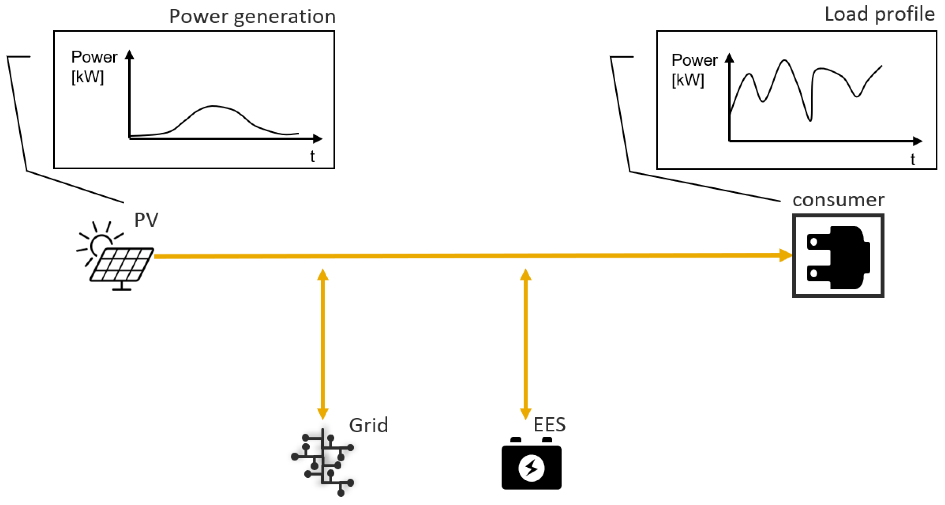
The system works as follows: consumers are supplied with electrical energy by the overall system, whereby the energy can potentially come from the photovoltaic modules (PV), the public electricity grid (PEG), or the battery (EES). Given exogenous PV production and load profiles (e.g., generated by historical or forecast data), the solver determines the cost-optimal size of the EES while deriving—and therefore also presuming—the optimal operating strategy for the overall system shown in Figure 9.

The bidirectional arrows mean that energy can be fed into as well as out of the component block, but not at the same timestep $t$. This is considered, for example, via exclusivity conditions in the constraints of the MILP formulations. The PV generation and demand data are historic data from a real industrial use-case for supplying electrical energy to a supermarket, which can vary over time, especially based on the season. The MG operator, in addition to selling the electrical energy to the supermarket, has certain cost and revenue blocks that must be weighed when operating the overall system and sizing the battery. Feeding PV energy into the PEG generates additional revenue, whereas demand from the PEG generates costs. These costs, in turn, consist of an energy (€/kWh) and a power price (€/kW_max); the second values the maximum demanded power in a timeframe with a cost factor. The feed-in tariff and the demand price in turn depend on the tariff structure and can fluctuate, for example, according to the region and the time of the day. These volatilities, both monetary and on the producer and consumer side, drive the advantageousness of a battery usage in such a system.

The question that arises is how big should the battery be that is chosen ($E^{max})$ to minimize the total cost (or maximize the profits). The decision is significantly influenced by the investment costs for the battery, the useful lifetime, and which technology—and accordingly which performance—the battery is based on. In parallel with charging and discharging efficiencies (%), performance is assessed primarily by the c-rate ($C$ in 1/h), which is defined as the ratio between maximum charging or discharging power and capacity. For lithium-ion batteries, 1C is usually used as a basis, which means that the battery can be fully charged in one hour. i.e., a linear relationship between state of charge $(SOC$ in %) and time. Therefore:

$$\frac{\partial C}{\partial SOC}=0, \forall SOC\in \left[0, 1\right]$$

(21)

For other technologies, the relationship (21) is not applicable anymore. Due to chemical processes in salt-nickel batteries, for example, (21) is no longer fulfilled. Furthermore, for these batteries the functional relationship $C=f\left(SOC\right)$ is nonlinear and not continuously differentiable [32]. At first glance, this seems unproblematic, since the univariate approximation methods in Section 2.2.2 can be used to approximately integrate these functional relationships into the MILP. However, since (21) is no longer fulfilled—independent of the other properties of the function—this has immediate consequences for the optimization program, since $C$ is no longer to be considered only as a parameter but as a variable.

The solver determines the cost-optimal values of the operational variables (e.g., optimal maximal (If (21) would be fulfilled, the maximal charging/discharge power could not vary by time) charging/discharge power $P_t^{max}$ and $SO{C}_t$ of the EES at each timestep) and the global variables (e.g., optimal size $E^{max}$ of the EES over the entire optimization horizon). By general definition for storage systems:

$$C_t=\frac{P_t^{max}}{E^{max}}, D_C=\{\left(P_t^{max}, E^{max}\right)\in {({ℝ}_0^{+})}^2 | E^{max}>0 \}$$

(22)

$$SO{C}_t=\frac{E_t}{E^{max}}, D_{SOC}=\{\left(E_t, E^{max}\right)\in {({ℝ}_0^{+})}^2 | E^{max}>0 \}$$

(23)

Since (22) and (23) each represent relationships between three variables, a quadratic-bivariate relationship exists. Although some solvers can handle quadratic nonlinearities, the linearization method used in this work can be applied to this situation in accordance with the relationship $z_t=f_a\left(x,y_t\right)$ from Section 2.3.2, where the indexed variables correspond to $y_t$. This allows a direct comparison between the solution of the nonlinear and the linearized problem and an evaluation of the presented method (Section 3.2). The resulting MIQCP problem can be solved with Gurobi, a commercially available standard solver. The solver uses the specific type of nonlinearity—quadratic in this case—to solve the problem exactly. This makes the computation much more efficient than using a general MINLP solver, setting a computationally efficient benchmark for the method being evaluated.

Both models—MIQCP and MILP—are implemented in Python (PyCharm Community Edition 2020.3.3) in the optimization environment Pyomo (Version 6.0.1) and solved by the Gurobi (Version 9.5.0) solver for $T=288$ and $\mathsf{\Delta }t=5 \left[\min \right]$.

3.2. Results and Evaluation

The relations (22) and (23) are integrated into the system from Section 3.1 using the method from Section 2. Solutions for different resolutions $n^x\ast n^y$ are compared with the MIQCP solution to evaluate the approximation quality, where the evaluation determinants are the optimal battery size $E_{max}$, computation time, and the relative error with respect to the objective value. For the meshing the following applies:

• $P_t^{max} \in \left[0, 1000\right]$ in kW;
• $E_t \in \left[0, 1000\right]$ in kWh;
• $E^{max} \in \left[1, 1000\right]$ in kWh.

Therefore, 1000 kWh is the predefined upper limit of the battery set by the person in charge, which should not be exceeded in any case, and the lower limit is 1 kWh, to avoid division by 0. The upper limits for $P_t^{max}$ and $E_t$ can be derived from this, since on the one hand the storage level can never be greater than the maximum capacity, and on the other hand, the maximum charging power is limited via the relationship $C=f\left(SOC\right)$ (Here, it is assumed that $C$ can have a maximum of 1/h. In this special case, the actual limit is even smaller and is considered through $C=f\left(SOC\right)$ in the system constraints). For different resolutions, we get different sizes for the overall model.

Table 1. Comparison of model size.

Case	# Variables	# Constraints
MIQCP	8.355 (4.611 C + 3.744 B) *	19,010
2 × 2	8.931 (4.611 C + 4.320 B)	22,466
3 × 3	10.659 (4.611 C + 6.048 B)	34,562
4 × 4	13.539 (4.611 C + 8.928 B)	54,722
5 × 5	17.571 (4.611 C + 12.960 B)	82,946
10 × 10	55.011 (4.611 C + 50.400 B)	345,026
15 × 15	121.251 (4.611 C + 116.640 B)	808,706
20 × 20	216.291 (4.611 C + 211.680 B)	1,473,986

* C = Continuous; B = Binary.

shows the model sizes with different resolutions and compares them with the MIQCP model without approximation constraints.

It can be seen that as the resolution increases, the model size increases significantly, which will be accompanied by increased computation time. Most notably, the number of binary variables also increases, which is related to the fact that as the resolution increases, the number of potential decision areas increases.

To solve the problems, two solver parameters have been manually adjusted in advance: the MIP gap is set to 0% and the maximum computation time to 2000 s. Furthermore, all solver parameters remain unchanged (“untuned”), whereby the default values of Gurobi are set automatically. This also includes the absence of manually set initial values for the optimization variables.

The benchmark is set by the MIQCP’s solution, with the optimal variable value for $E_{max}$, the relative error, and the computation time in

Table 2. Comparison of solving performance for Windows 10 × 64 with 8 GB RAM and Intel(R) Core (TM) i5-10210U CPU @ 1.60 GHz, 2112 MHz, 4 cores, and 8 logical processors.

Case	Emax [kWh]	Error * [%]	Time [s]	Gap [%]
MIQCP	741.6989	0	36.74	0
2 × 2	infeasible	-	-	-
3 × 3	720.16	0.58	4.66	0
4 × 4	724.15	0.22	2.56	0
5 × 5	750.25	0.08	40.16	0
10 × 10	724.3	0.18	149.99	0
15 × 15	721.84	0.08	610.79	0
20 × 20	723.24	0.17	terminated	0.29

* Relative error defined as $\frac{\left|{\mathrm{F}}^{\mathrm{MIQCP}}-{\mathrm{F}}^{\mathrm{A}}\right|}{{\mathrm{F}}^{\mathrm{MIQCP}}}$.

. The approximation quality is measured by the relative error, which measures the deviation between the “true” optimal objective value $F^{\mathrm{MIQCP}}$ and the approximated optimal objective value $F^A$. Computation time, on the other hand, is the efficiency measure. As a trend, it can be observed that as the resolution increases, the error decreases, but at the expense of computation time. This is not surprising, and the user has to find the best compromise for the individual case. It is noticeable that the model is not solvable for a 2 × 2 resolution (geometrically a surface with only one area; Figure 5). This is because of the too strong restriction of the solution space, since the optimizer has only one area available and is forced into it. With the 3 × 3 resolution, there are already four areas available in each timestep for the solver to choose from, making the solution space larger and the model feasible. However, the error is large compared to the higher resolution cases. With the 5 × 5 resolution, the computation time of the approximation exceeds the one of the MIQCP formulation for the first time. However, the error of 0.08% is comparatively small and does not tend to decrease at higher resolutions. With the 20 × 20 resolution, the second termination criterion—besides the MIP gap—comes into effect, and the computation is terminated after 2000 s, with a remaining MIP gap of 0.29%. Considering the results for the resolutions presented here, the 5 × 5 resolution is the best performing one based on accuracy and efficiency. It should be mentioned at this point that the results should only be interpreted in the context of the specific use-case and any numerical errors should be considered.

What also strikes us is that $E_{max}$ (the variable of interest) deviates in the order of 10¹ from the value assigned to the variable in the MIQCP case. This means that although the object value is approximated fairly accurately and the approximation quality can be increased with increasing resolution, the solution path, i.e., the assignment of values to the individual variables to achieve the object value, can deviate significantly. From this, one can deduce that the battery size can only be determined in the context of the underlying approximation case and is not useful for comparison. This is mainly due to the fact that the other variables—which will not be discussed further in this context—also take different values depending on the respective case. Therefore, the optimal value for the battery is only optimal in combination with the other values of the variables. This once again illustrates the dependency of sizing and scheduling as mentioned in the introduction.

In the previous section, it is mentioned what the objective function—which is a cost function—is composed of. If, hypothetically, only the battery size $E_{max}$ would be a variable in the objective function, the size would differ only by the relative error from case to case, since that would be the only variable affecting the objective function value.

The results suggest good performance also for other MINLPs—and not only MIQCPs as a special case—since the approximation itself does not depend on the type of nonlinearity.

4. Conclusions and Outlook

In this work, a detailed approach has been developed to integrate nonlinear-bivariate functions in MILP environments. On the one hand, the methodological, theoretical framework is created and formulated in detail. On the other hand, the performance is evaluated on the basis of a real use-case. This closes the research gap between generic approximation approaches and problem-specific formulations by means of a general-practical approach, whereby the concrete implementation is provided via a source code in the Supplementary Materials. The results in Table 2 show that the method provides satisfactory results in terms of both accuracy (error 0.08%) and efficiency (9% longer computation time), even for a conservative comparison with efficient off-the-shelf MIQCP solvers like Gurobi. However, it is important to keep in mind that these results should always be interpreted in the context of the specific use-case. In this paper, this is the MIQCP approximation for a defined MG or battery sizing problem. Accordingly, other nonlinear formulations or systems and problems may lead to different results, but this requires further research. However, the results suggest that a similar performance can be achieved for other MINLPs, since the type of nonlinearity does not matter for the approximation.

In addition to other use-cases, both in terms of system topology and problem as well as the nature of the bivariate nonlinearity, this work can also serve as a starting point for further research and methodological extensions. In Section 2.2.1, equally distributed breakpoints are introduced. As mentioned earlier, in some cases it may make sense to distribute breakpoints unequally, whether manually or algorithmically. One algorithmic possibility is, for example, to discretize the function with a high resolution and to determine the slopes between the points. Then, one can sort the slopes by magnitude and distribute a defined number of breakpoints around the points with the largest slopes. However, for a reasonable distribution, the shape—especially the directional changes—of the function must also be considered. In addition to the position, the adequate number of breakpoints can also be determined algorithmically rather than a priori; further content can, for example, be found in Lin et al. [33] and Asghari et al. [34].

Another extension could be to remove the assumption of constancy (11) for each area which leads to (18) and (19) being linear. This is achieved by approximating PWL in one variable domain and PWC in the other. However, as we see, Gurobi is capable of solving MIQCPs very efficiently. It would therefore be possible to transform (18) and (19) from a linear to a quadratic expression, potentially increasing the accuracy of the approximation of general nonlinear problems (not just MIQCP). Thus, the slope depends on the position within an area and is no longer constant for the respective area. Of course, this assumes that the slope is a linear function of the variables, which can be achieved, for example, by a PWL approximation for both domains.

References

1. Eto, J.; Lasseter, R.; Klapp, D.; Khalsa, A.; Schenkman, B.; Illindala, M.; Baktiono, S. The CERTS Microgrid Concept, as Demonstrated at the CERTS/AEP Microgrid Test Bed; Ernest Orlando Lawrence Berkeley National Laboratory: Berkeley, CA, USA, 2018.
2. Abel, D.; Neisen, V.; Baader, F. Supervisory Model-based Control using Mixed Integer Optimization for stationary hybrid fuel cell systems. IFAC-PapersOnLine 2018, 51, 320–325. [Google Scholar] [CrossRef]
3. Kotzur, L.; Markewitz, P.; Robinius, M.; Stolten, D. Kostenoptimale Versorgungssysteme für ein vollautarkes Einfamilienhaus. In 10. Internationale Energiewirtschaftstagung IEWT Wien 2017; Institute of Electrochemical Process Engineering, Forschungszentrum Jülich GmbH: Jülich, Germay, 2016. [Google Scholar]
4. Jaramillo, L.; Weidlich, A. Optimal microgrid scheduling with peak load reduction involving an electrolyzer and flexible loads. Appl. Energy 2016, 169, 857–865. [Google Scholar] [CrossRef]
5. Jochem, P.; Schönfelder, M.; Fichtner, W. An efficient two-stage algorithm for decentralized scheduling of micro-CHP units. Eur. J. Oper. Res. 2015, 245, 862–874. [Google Scholar] [CrossRef] [Green Version]
6. Fontenot, H.; Dong, B. Modeling and control of building-integrated microgrids for optimal energy management—A review. Appl. Energy 2019, 254, 113689. [Google Scholar] [CrossRef]
7. García Vera, Y.; Dufo-López, R.; Bernal-Agustín, J. Energy Management in Microgrids with Renewable Energy Sources: A Literature Review. Appl. Sci. 2019, 9, 3864. [Google Scholar] [CrossRef] [Green Version]
8. Klanšek, U. A comparison between MILP and MINLP approaches to optimal solution of Nonlinear Discrete Transportation Problem. Transport 2015, 30, 135–144. [Google Scholar] [CrossRef] [Green Version]
9. Ipopt Documentation. Available online: https://coin-or.github.io/Ipopt/ (accessed on 7 February 2022).
10. SCIP Solving Constraint Integer Programs. Available online: https://scipopt.org/ (accessed on 7 February 2022).
11. BARON Solver. Available online: https://minlp.com/baron-solver (accessed on 7 February 2022).
12. Gurobi Optimizer. Available online: https://www.gurobi.com/products/gurobi-optimizer/ (accessed on 7 February 2022).
13. Bussieck, M.; Vigerske, S. MINLP Solver Software. In Wiley Encyclopedia of Operations Research and Management Science; Wiley: Hoboken, NJ, USA, 2011. [Google Scholar] [CrossRef]
14. Floudas, C. ANTIGONE. 2013. Available online: https://www.gams.com/latest/docs/S_ANTIGONE.html (accessed on 3 June 2022).
15. Lindo Systems, Inc. LINDOGlobal. Available online: https://www.gams.com/latest/docs/S_LINDO.html (accessed on 3 June 2022).
16. Octeract Optimisation Intelligence. Octeract Engine. Available online: https://www.gams.com/latest/docs/S_OCTERACT.html (accessed on 3 June 2022).
17. Kallrath, J. Gemischt-Ganzzahlige Optimierung: Modellierung in der Praxis. Mit Fallstudien aus Chemie, Energiewirtschaft, Papierindustrie, Metallgewerbe, Produktion und Logistik; Springer: Berlin/Heidelberg, Germany, 2013. [Google Scholar] [CrossRef]
18. Alarie, S.; Audet, C.; Gheribi, A.; Kokkolaras, M.; LeDigab, S. Two decades of blackbox optimization applications. EURO J. Comput. Optim. 2021, 9, 100011. [Google Scholar] [CrossRef]
19. Kaur, S.; Kumbhar, G.; Sharma, J. A MINLP technique for optimal placement of multiple DG units in distribution systems. Electr. Power Energy Syst. 2014, 63, 609–617. [Google Scholar] [CrossRef]
20. Shi, H.; You, F. Energy Optimization of Water Supply System Scheduling: Novel MINLP Model and Efficient Global Optimization Algorithm. AIChE J. 2016, 62, 4277–4296. [Google Scholar] [CrossRef]
21. Elsido, C.; Bischi, A.; Silva, P.; Martelli, E. Two-stage MINLP algorithm for the optimal synthesis and design of networks of CHP units. Energy 2017, 121, 403–426. [Google Scholar] [CrossRef]
22. Taccaria, L.; Amaldia, E.; Martelli, E.; Bischi, A. Short-Term Planning of Cogeneration Power Plants: A Comparison between MINLP and Piecewise-Linear MILP Formulations. Comput. Aided Chem. Eng. 2015, 37, 2429–2434. [Google Scholar] [CrossRef]
23. D’Ambrosio, C.; Lodi, A.; Martello, S. Piecewise linear approximation of functions of two variables in MILP models. Oper. Res. Lett. 2010, 38, 39–46. [Google Scholar] [CrossRef]
24. Kelley, M.; Pattison, R.; Baldick, R.; Baldea, M. An efficient MILP framework for integrating nonlinear process dynamics and control in optimal production scheduling calculations. Comput. Chem. Eng. 2018, 110, 35–52. [Google Scholar] [CrossRef]
25. Rebennack, S.; Kallrath, J. Continuous Piecewise Linear Delta-Approximations for Bivariate and Multivariate Functions. J. Optim. Theory Appl. 2015, 167, 102–117. [Google Scholar] [CrossRef]
26. Fügenschuh, A.; Hayn, C.; Michaelis, D. Mixed-integer linear methods for layout-optimization of screening systems in recovered paper production. Optim. Eng. 2014, 15, 533–573. [Google Scholar] [CrossRef]
27. Adams, W.; Sherali, H. Linearization Strategies for a Class of Zero-One Mixed Integer Programming Problems. Oper. Res. 1990, 38, 217–226. [Google Scholar] [CrossRef]
28. Bischi, A.; Taccari, L.; Martelli, E.; Amaldi, E.; Manzolini, G.; Silva, P.; Campanari, S.; Macchi, E. A detailed MILP optimization model for combined cooling, heat and power system operation planning. Energy 2014, 74, 12–26. [Google Scholar] [CrossRef]
29. Cheng, C.; Wang, J.; Wu, X. Hydro Unit Commitment with a Head-Sensitive Reservoir and Multiple Vibration Zones Using MILP. IEEE Trans. Power Syst. 2016, 31, 4842–4852. [Google Scholar] [CrossRef]
30. Tong, B.; Zhai, Q.; Guan, X. An MILP Based Formulation for Short-Term Hydro Generation Scheduling with Analysis of the Linearization Effects on Solution Feasibility. IEEE Trans. Power Syst. 2013, 28, 3588–3599. [Google Scholar] [CrossRef]
31. Wu, Z.; Ding, J.; Wu, Q.; Jing, Z.; Zheng, J. Reserve constrained dynamic economic dispatch with valve-point effect: A two-stage mixed integer linear programming approach. CSEE J. Power Energy Syst. 2017, 3, 203–211. [Google Scholar] [CrossRef]
32. Technical Questions. Available online: https://www.innov.energy/en/faqs/salt-battery/technique (accessed on 21 February 2022).
33. Lin, M.; Carlsson, J.; Ge, D.; Shi, J.; Tsai, J. A Review of Piecewise Linearization Methods. Math. Probl. Eng. 2013, 2013, 101376. [Google Scholar] [CrossRef] [Green Version]
34. Asghari, M.; Fathollahi-Fard, A.M.; Mirzapour Al-e-hashem, S.M.J.; Dulebenets, M.A. Transformation and Linearization Techniques in Optimization: A State-of-the-Art Survey. Mathematics 2022, 10, 283. [Google Scholar] [CrossRef]
Figure 1. Architectonic design.
Mathematics 10 02226 g001
Figure 2. Top view of the surface on the example of a 5 × 5 resolution for z = f ( x ,   y ) .
Mathematics 10 02226 g002
Figure 3. PWC (z = f(x)) and PWL (z = f(y)) approximation, with k = 1 ,   ,   ( n x 1 ) and l = 1 ,   ,   ( n y 1 ) . The two newly introduced indices k and l index the areas, whereas i and j are used to index the breakpoints and function values (Section 2.2.1). By selecting the area k or l, the upper and lower limits stored in x, y, and z can be accessed (Section 2.3.1).
Mathematics 10 02226 g003
Figure 4. Exemplary approximation mesh of z = f ( x ,   y ) = y log ( x ) with 10 × 10 resolution.
Mathematics 10 02226 g004
Figure 5. Area k , l of the approximation mesh.
Mathematics 10 02226 g005
Figure 6. Exemplary determination of the approximative function value z = f a ( x , y ) with a 5 × 5 resolution.
Mathematics 10 02226 g006
Figure 7. Exemplary determination of the approximative function value z t = f a ( x t , y t ) with a 5 × 5 resolution for multiple timesteps.
Mathematics 10 02226 g007
Figure 8. Exemplary determination of the approximative function value z t = f a ( x , y t ) with a 5 × 5 resolution for multiple timesteps.
Mathematics 10 02226 g008
Figure 9. System topology of the microgrid (the use-case MG resulted from project work, mentioned in the Acknowledgments).
Mathematics 10 02226 g009