Combining Key-Points-Based Transfer Learning and Hybrid Prediction Strategies for Dynamic Multi-Objective Optimization

Abstract

Dynamic multi-objective optimization problems (DMOPs) have been of interest to many researchers. These are problems in which the environment changes during the evolutionary process, such as the Pareto-optimal set (POS) or the Pareto-optimal front (POF). This kind of problem imposes more challenges and difficulties for evolutionary algorithms, mainly because it demands population to track the changing POF efficiently and accurately. In this paper, we propose a new approach combining key-points-based transfer learning and hybrid prediction strategies (KPTHP). In particular, the transfer process combines predictive strategy with obtaining anticipated key points depending on the previous moments to acquire the optimal individuals at the new instance during the evolution. Additionally, center-point-based prediction is used to complement transfer learning to comprehensively generate initial populations. KPTHP and six state-of-the-art algorithms are tested on various test functions for MIGD, DMIGD, MMS, and HVD metrics. KPTHP obtains superior results on most of the tested functions, which shows that our algorithm performs excellently in both convergence and diversity, with more competitiveness in addressing dynamic problems.

1. Introduction

The field of multi-objective optimization has always received a lot of attention from researchers. Multi-objective optimization problems (MOPs) [1,2] are dedicated to optimizing multiple objectives simultaneously to obtain an approximate optimal solution. They have a wide range of applications, including environmental applications [3], biology [4], space robots [5], and energy allocation [6,7]. Multi-objective evolutionary algorithms (MOEAs) [8,9,10,11,12] are considered an efficient choice to deal with MOPs by finding the most plausible individuals in the objective space to compose the POS. The function value of the POS in the objective space is called the POF [13,14].

There are two kinds of multi-objective optimization problems in total, including static multi-objective optimization problems (SMOPs) and dynamic multi-objective optimization problems (DMOPs). Compared with SMOPs, DMOPs have more difficulties and challenges, because their POS or POF shape changes with time and is irregular in many cases. Accordingly, dynamic multi-objective optimization algorithms (DMOAs) are powerful tools for solving DMOPs and are widely employed to solve many real-life problems. Common application areas include scheduling [15,16,17], control [18], chemistry [19], industry [20], and energy design [21]. For example, when solving vehicle routing problems for package delivery, not only do the number of vehicles, path lengths, and other objectives need to be optimized in a static manner, but the time window of customers and the dynamically changing topology of customers should be considered to satisfy the needs of practical scenarios [22]. There are two basic requirements to solve DMOPs. The first is to accurately identify changes and then react to them. Many efficient identification mechanisms [23,24] have now been proposed. The second is a dynamic response mechanism [25,26]. When the environment changes, the algorithm is capable of tracing the POF quickly and precisely according to the type of change. In this paper, we consider the environment to be constantly changing, thus mainly concentrating on dynamic response mechanisms.

According to the description in [27], DMOPs can be classified into four types based on whether the POF or POS varies. The specific classification is as follows. Type I indicates that the POS changes but the POF stays the same. Type II denotes that both POF and POS change. Type III represents that the POF changes and the POS remains unchanged. Type IV means that both POS and POF remain unchanged. For the fourth type, there is not much research significance. According to the above type classification, DMOPs can be divided into two categories: predictable-change and unpredictable-change problems [28]. In predictable-change problems, the POF or POS have a certain similarity and regularity through the continuous environmental changes, and the response can be adjusted or predicted according to the previous POS and POF. However, in unpredictable-change problems, the POF changes irregularly and is likely to change very drastically, which means that strategies such as simple prediction will yield very poor results.

There are numerous algorithms and mechanisms to deal with DMOPs, and the most common strategies are prediction-based methods and diversity-maintenance-based methods. It is well recognized that prediction-based methods can accelerate convergence [29,30,31], but for unpredictable changes, the accuracy and validity of the prediction are dramatically reduced, resulting in the loss of diversity. Therefore, diversity-maintaining-based methods are essential [32]. Nowadays, most of the algorithms’ strategies are limited to simply improve convergence or maintain diversity. Based on the above analysis, a prediction-based approach and an approach based on maintaining diversity can be perfectly integrated so that both rapid convergence and good diversity maintenance can be achieved concurrently. With these thoughts in mind, we propose a new response mechanism that combines key-points-based transfer learning and hybrid prediction strategies (KPTHP).

In this paper, key-points-based transfer learning is adept at coping with unpredictable changes, and it focuses on transferring based on three types of key points: the center point, the polar point, and the boundary point. The transfer process can respond perfectly and quickly to nonlinear changes, and on the contrary, the center-point-based prediction has more advantages in solving linear changes. Consequently, the integration of key-points-based transfer learning and hybrid prediction makes full use of their strengths to make more accurate transfers and predictions and accelerates responding to different types of predictable changes. Experimental results on various test functions demonstrate that KPTHP is very competitive in handling problems with different dynamic characteristics, obtaining better convergence and diversity.

The contributions of this paper are summarized as follows:

(1)

Key-points-based transfer learning exploits the predicted key points to guide the future search process and the evolution of the population, filtering out partial high-quality individuals with better diversity. As a result, it can cope with nonlinear environmental changes with high efficiency, exploring the most promising optimization space in decision space and decreasing the probability of negative transfer caused by drastic environmental changes.

(2)

The center-point-based prediction strategy not only can respond quickly to the same successive environmental changes but also has the flexibility to tackle two environmental changes that are similarly distributed or partially different. It adopts a first-order feed-forward difference linear model to anticipate the positions of the individuals at the next moment, which in turn complements key-points-based transfer learning to attain excellent convergence.

The remainder of the paper is structured as follows. Section 2 presents the background, including some basic concepts and related work. The proposed KPTHP is described in detail in Section 3. Section 4 introduces the configurations, the results, and analysis of the experiments in terms of different test functions. The algorithms are further discussed in Section 5. Finally, conclusions are drawn in Section 6.

2. Background

2.1. Dynamic Multi-Objective Optimization

The intrinsic feature of DMOPs is that the objective value changes over time as the environment changes. A general definition of a dynamic multi-objective problem can be as follows:

$$\begin{array}{c}Minimize F(x,t)=<f_1(x,t),f_2(x,t),\dots ,f_m(x,t)>,\\ s.t. x\in \Omega \end{array}$$

(1)

where x =< x₁, x₂, …, x_n> is the n-dimensional decision variable and $\Omega \subset R^n$ is the decision space. $\Omega =[L_1,U_1]\times [L_2,U_2]\times \cdots \times [L_n,U_n]$. $L_i,U_i\in R^n$ are the lower and upper bounds of the ith decision variable, respectively. $f_1,f_2,\dots ,f_m$ are objective functions, and m is the objective number. t is a time variable representing the dynamic nature of the problem.

Definition 1 (Dynamic Decision Vector Domination).

For any two decision vectors x₁ and x₂ at time t, x₁ dominates x₂, denoted by$x_1{\succ }_t{x}_2$, only when the following conditions are satisfied:

$$\{\begin{array}{ll}{f}_i(x_1,t)\le f_i(x_2,t)& \forall i=1,\dots ,m\\ f_i(x_1,t)<f_i(x_2,t)& \exists i=1,\dots ,m\end{array}$$

(2)

Definition 2 (Dynamic Pareto-Optimal Set (DPOS)).

Both x₁ and x₂ are decision vectors. If a solution x* is not dominated by any of the solutions x in the decision space at moment t, then x* is called a non-dominated solution. All the non-dominated solutions at time t are called POS in the decision space, and the set of dynamic Pareto-optimal solutions is called the DPOS. The representation is as follows:

$$DPOS=\left\{x^{*}\right|\neg \exists x\in \Omega :x{\succ }_t{x}^{*}\}$$

(3)

Definition 3 (Dynamic Pareto-Optimal Front (DPOF)).

DPOF is the corresponding object vector of DPOS at moment t. The mathematical form is defined as:

$$DPOF=\left\{y^{*}\right|y^{*}=F(x^{*},t),x^{*}\in DPOS\}$$

(4)

2.2. Related Works

In recent years, many advances have been accomplished in the field of DMOPs. There are many existing methods, which can be primarily divided into the following categories depending on the behavior of the algorithms: prediction-based, memory-based, and diversity-based methods.

2.2.1. Prediction-Based Methods

Generally speaking, if the dynamics of DMOPs are predictable or regular, prediction-based methods can reuse past information to forecast the location of the optimal solution at the next moment. Therefore, the optimal solution obtained can be quickly converged to the new POF. For example, Hatzakis and Wallace [33] described a forward-looking approach for the solution of time-changing problems (FPS). The prediction model is built using a priori optimal sequences of position, from which the next position can be estimated. Zhou et al. [34] proposed a method for predicting the entire population by considering the attributes of successive dynamic multi-objective problems, called the population prediction strategy (PPS), in which the individuals are predicted by combining the predicted center point and the evaluated manifold. Muruganantham et al. [35] proposed a new dynamic MOEA using Kalman filter predictions (MOEA/D-KF) in decision space, and this prediction method facilitates guiding the search process towards the optimal solution.

Jiang and Yang [36] presented a steady-state and generational evolutionary algorithm (SGEA) for efficiently handling DMOPs, and the main novelty is that it reuses a percentage of out-of-date solutions with good distribution and relocates some solutions close to the new Pareto front on the basis of information collected from the previous environment and the new environment. Wang et al. [37] proposed a predictive method based on grey prediction model (GM-DMOP). The algorithm builds the grey prediction model by using the centroid point of each cluster when detecting the environmental change and then generates the initial population. Zou et al. [30] presented a knee-guided prediction approach (KPEA) to predict population more effectively.

2.2.2. Memory-Based Methods

Memory-based methods usually store the previous optimal solutions and keep them updated [38,39]. When the environment changes mildly or similarly to the previous environment, the optimal solutions in the storage space are reintroduced to improve the performance of the algorithm and accelerate the convergence. Existing research suggests that memory-based mechanisms are generally adopted to deal with environments that change periodically [40]. Goh and Tan [41] proposed a dynamic competitive–cooperative coevolutionary algorithm (dCOEA), which incorporates the features of temporal memory to exploit past information and stochastic competitors to track the changing solution set. Zheng et al. [42] presented a population-diversity-maintaining strategy based on a dynamic environment evolutionary model (DEE-PDMS). This strategy takes advantage of the dynamic environment to store different knowledge and information generated by population before and after environmental change, and correspondingly, the knowledge and information guide the evolution in the new environment.

Zhang et al. [43] proposed a cluster-based clonal selection algorithm for global optimization (CCSA), in which a memory mechanism is presented to deposit the previous searching information and reused for optima tracking. Chen et al. [44] implemented a dynamic two-archive evolutionary algorithm that maintains two co-evolving populations simultaneously (DTAEA). In this algorithm, the two populations are complementary to each other, and one population concerns mainly the convergence, while the other concerns mainly the diversity. Liang et al. [45] proposed a hybrid of memory and prediction strategies (HMPS). In HMPS, if changes are monitored that are similar to previous changes, memory-based methods are used to relocate individuals in the new environment. Hu et al. [46] suggested a novel evolutionary algorithm based on the intensity of environmental change (IEC). In this algorithm, a memory mechanism is introduced that keeps individuals of the current optimization population equal according to the distribution of the vector.

2.2.3. Diversity-Based Methods

The diversity-based approach consists mainly of diversity introduction and diversity maintenance. The former is mainly devoted to enabling previously converged populations to jump out of their current position to explore new regions. The latter aims to maintain the intrinsic diversity of the population in the evolutionary optimization process. Woldesenbet and Yen [47] proposed a new dynamic evolutionary algorithm that uses variable relocation to converge or evolve in the new environmental condition (RVDEA), where relocation radius introduces a certain amount of uncertainty to be applied specifically for each individual to sustain diversity. Kwong et al. [48] designed a dynamic neighborhood multi-objective evolutionary algorithm based on hypervolume indicator (DNMOEA/HI), in which the hypervolume indicator is utilized to guide diversity preservation. Azzouz et al. [49] used reference vectors to ensure the guidance of the search towards the POF and thus maintain diversity.

Gong et al. [50] proposed a framework of dynamic interval multi-objective cooperative co-evolutionary optimization based on the interval similarity (DI-MOPs). They employed a technique based on change intensity and a random mutation strategy to track the changing Pareto front. Wang et al. [51] proposed a prediction method that incorporates the Gaussian Mixture Model (GMM) into the MOEA/D framework (MOEA/D-GMM). They employed a powerful non-linear model to accurately fit various data distributions. Zou et al. [28] proposed a hybrid prediction strategy and a precision-controllable mutation strategy (HPPCM) to solve the DMOPs. In the approach, the precision-controllable mutation strategy can effectively handle unpredictable environmental changes to improve the diversity exploration of the population.

In addition to the three types of methods mentioned above, there are some extraordinary methods based on machine learning and reinforcement learning mechanisms [52,53,54]. Zou et al. [55] proposed a dynamic multi-objective evolutionary algorithm driven by inverse reinforcement learning. This algorithm uses limited data to accomplish a promising evolutionary process and to guide the search for populations. Jiang et al. [56] proposed an algorithmic framework called transfer-learning-based dynamic multi-objective evolutionary algorithm (Tr-DMOEA), which integrates transfer learning and population-based evolutionary algorithms to solve DMOPs. Similarly, there is reducing negative transfer learning via clustering for dynamic multi-objective optimization algorithm (CT-DMOEA) [57] and so on. Cao et al. [58] presented a support vector regression-based prediction algorithm (MOEA/D-SVR) to generate the initial population in the new environment, and the basic idea of this predictor is to map the historical solutions into a high-dimensional feature space via a nonlinear mapping and to perform linear regression in this space.

3. Proposed KPTHP

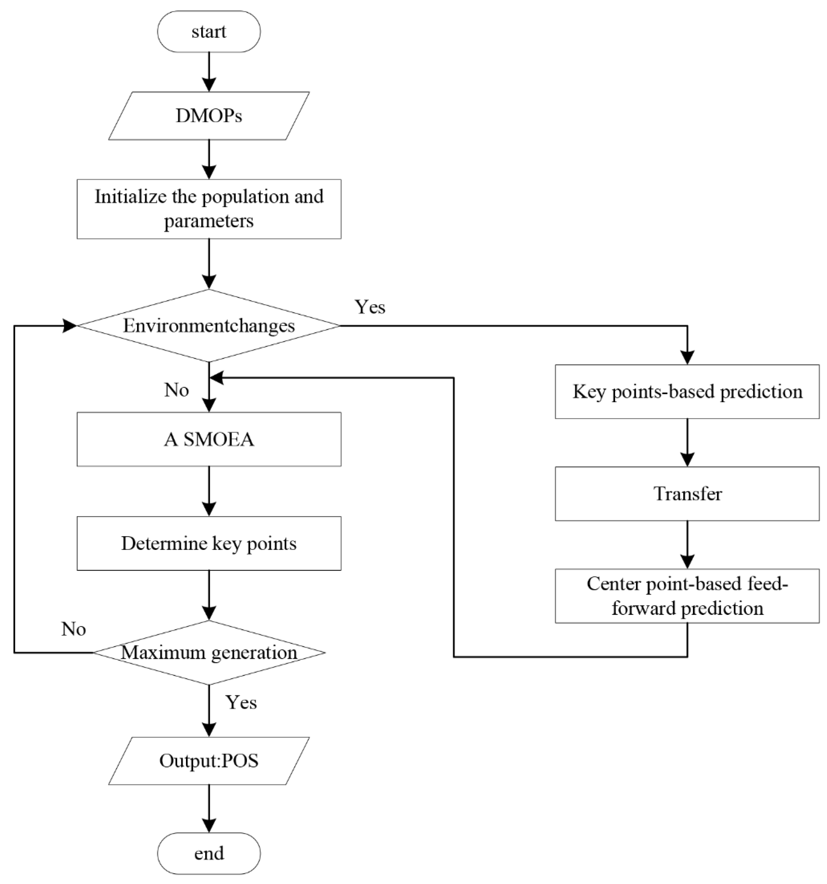
In this section, we introduce the details of the proposed KPTHP. Figure 1 depicts the KPTHP procedure. To be specific, the framework of the proposed algorithm is outlined first. Afterwards, the details of determining key points, key-points-based prediction, transfer, and center-point-based feed-forward prediction in the framework are described. Finally, we analyze the computational complexity of proposed KPTHP.

3.1. Overall Framework

The main framework of the KPTHP is presented in Algorithm 1. When the environment change is detected, during the first two changes, we use a static multi-objective optimization evolutionary algorithm (SMOEA) [59,60,61] to evolve. In the changes that follow, we first determine the key points predicted (Algorithms 2 and 3) for transfer (Algorithm 4) at moment t to obtain portion of high-quality individuals and then derive center-point-based predicted individuals using feed-forward prediction model (Algorithm 5). The transferred individuals and the predicted individuals are merged to form the initial population. Following every evolution, we are required to identify the key points of POS (Algorithm 2).

Algorithm 1: The overall framework of KPTHP

Input: The dynamic problem Ft(x), the size of the population: N, a SMOEA.

Output: The POS of the Ft(x) at the different moments.

Initialize population and related parameters;

while the environment has changed do

if t == 1 || t == 2 then

Initialize randomly the population initPop;

POSt = SMOEA(initPop, Ft(x), N);

KPointst = DKP(POSt, Ft(x), N);

Generate randomly dominated solutions Pt;

Else

PreKPointst = KPP(KPointst−1, KPointst−2);

TransSol = TF(POSt−1, PreKPointst);

FeeforSol = CPFF(POSt−1, KPointst−1, KPointst−2);

POSt = SMOEA(TransSol, FeeforSol, Ft(x), N);

KPointst = DKP(POSt, Ft(x), N);

Generate randomly dominated solutions Pt;

end if

t = t + 1;

return POSt;

end while

3.2. Determine Key Points

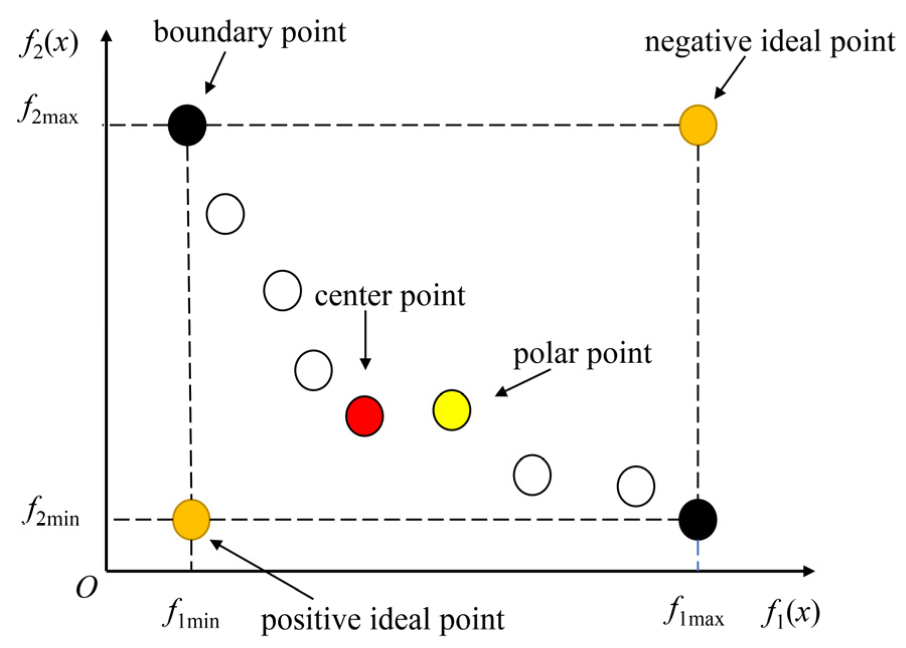
Many researchers have tried to identify special points on the POF that have considerable properties or represent local features of the POF. There are several types of points that have received more attention, including the center point, the boundary point, the ideal point, and the knee point. In this section, we mainly select three types of key points for the subsequent transfer and feed-forward prediction process, which are the center point, the boundary point, and the ideal point. The schematic diagram of the key points is shown in Figure 2. The center point is located at the center of the population, and the ideal point and boundary points can maintain the perimeter and boundary of the population, collectively reflecting the overall situation of the population. The concept and method of deriving the three types of key points are as follows.

Let POS_t = [39] be the Pareto-optimal set at t moment. The center point [62] of POS_t could be estimated by

$$Centers=\frac{1}{\left|PO{S}_t\right|}{\displaystyle \sum _{x_t\in PO{S}_t}{x}_t}$$

(5)

For the minimization problem, the boundary point is the individual with the smallest target value in one dimension of the target space. The number of the boundary point is determined by the dimension of the target space. If the dimension of the target space is 2, then the number of boundary points is 2, and the same is true for higher dimensions.

$$Boundary{s}_d=\min \{PO{F}_{td}^1,PO{F}_{td}^2,\dots ,PO{F}_{td}^p\}$$

(6)

where p is the number of the Pareto-optimal solution at the current moment t. $PO{F}_{td}^n$ denotes the Pareto front value in the d dimension of the target space at moment t.

$$Boundarys=\left\{Boundary{s}_d\right\},\hspace{1em}d\in \{1,2,\dots ,m\}$$

(7)

where m indicates the dimension of the target space. The set of the boundary point Boundarys consists of the boundary points of each dimension.

Ideal points are classified as positive and negative ideal points, and they are defined as follows. The positive point $z^{pi}=(z_1^{pi},z_2^{pi},\dots ,z_m^{pi})$, where $z_i^{pi}$ is the maximum of f_i(x), $x\in PO{S}_t$ for every $i\in \{1,2,\dots ,m\}$. The negative point $z^{ni}=(z_1^{ni},z_2^{ni},\dots ,z_m^{ni})$, where $z_i^{ni}$ is the minimum of f_i(x), $x\in PO{S}_t$ for every $i\in \{1,2,\dots ,m\}$. It is worth noting that the ideal point we use in this paper is the near-ideal point called the polar point. The procedure for solving the polar point is as described below.

Algorithm 2: Determine key points (DKP)

Input: The dynamic problem Ft(x), Pareto-optimal set POSt at the moment t, the size of the population N.

Output: Obtained key points KPointst in POSt.

KPointst = ∅

Calculate the center points Centers in each dimension according to Formula (5);

Obtain POFt of each non-dominated solution in POSt;

Compute the minimum value of each dimension in POFt;

Determine boundary points Boundarys according to Formula (7);

Determine the polar point Ideals by using the TOPSIS method;

KPointst = Centers $\cup$ Boundarys $\cup$ Ideals;

return KPointst;

In this section, we choose TOPSIS method [63,64] to obtain the polar point. First, TOPOSIS calculates the weighted decision matrix and determines the positive ideal solution and negative ideal solution. Afterwards, the grey correlations d⁺ d⁻ between each individual and the positive and negative ideal solution are calculated, respectively. Finally, the grey correlation occupancy DS of each individual was calculated according to Formula (8), and the individual with the largest DS value was selected. Algorithm 2 describes the strategy of determining key points.

$$DS=\frac{d^{+}}{d^{+}+d^{-}}$$

(8)

Algorithm 3: Key-points-based prediction (KPP)

Input: Key points KPointst−1 and KPointst−2 at moment t − 1 and t − 2.

Output: Predicted key points PreKPointst at moment t.

Determine the evolutionary direction between the key points by (9);

Obtain predicted key points PreKPointst at moment t by (10);

Add Gaussian noise with individuals in PreKPointst to PreKPointst;

return PreKPointst;

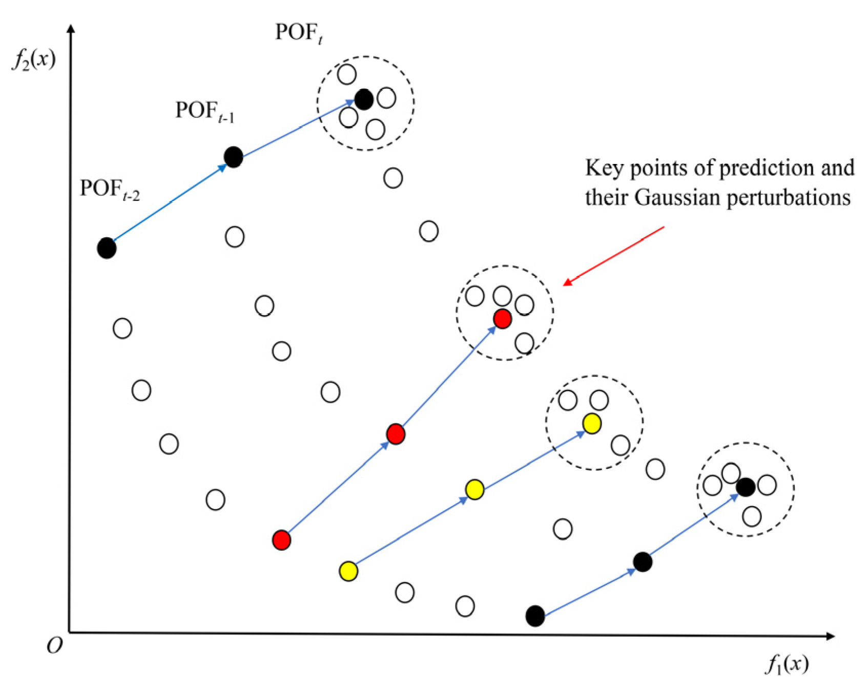
3.3. Key-Points-Based Prediction

For solving DMOPs, many methods based on some special regions or points on the POF have been designed [29,65]. In this section, the key points we consider are the center point, the boundary point, and the polar point. The center point shows the average characteristics of the whole population, and the boundary point and the polar point maintain the diversity of population, which can make the predicted population track POF more precisely and improve the convergence speed toward the POF. Figure 3 shows the process of prediction based on key points.

According to Algorithm 3, once the key points at time t − 1 and t − 2 are determined, they will be used to obtain the key points at time t. The process of solving is given as follows. First of all, we need identify key points KPoints_t−1 and KPoints_t−2 in POS_t−1 and POS_t−2. Thereafter, the distance between the key points is calculated by the following formula, respectively.

$$\Delta k=KPoint{s}_{t-1}-KPoint{s}_{t-2}$$

(9)

With Formula (9), each key point can determine an evolutionary direction for itself. Furthermore, the key points at time t can be predicted by Formula (10):

$$KPoint{s}_t=KPoint{s}_{t-1}+\Delta k$$

(10)

Finally, based on Formula (11), we add Gaussian noise with individuals in KPoints_t:

$$KPoint{s}_t=KPoint{s}_t+Gauss(0,\delta )$$

(11)

where Gauss(0, δ) indicates the Gaussian perturbation with mean 0 and standard deviation δ. Here, δ is defined as:

$$\delta =\frac{\left|\right|KPoint{s}_{t-1}-KPoint{s}_{t-2}\left|\right|}{n}$$

(12)

where $\left|\right|KPoint{s}_{t-1}-KPoint{s}_{t-2}\left|\right|$ is the Euclidean distance between KPoints_t−1 and KPoints_t−2 and n is size of the search space.

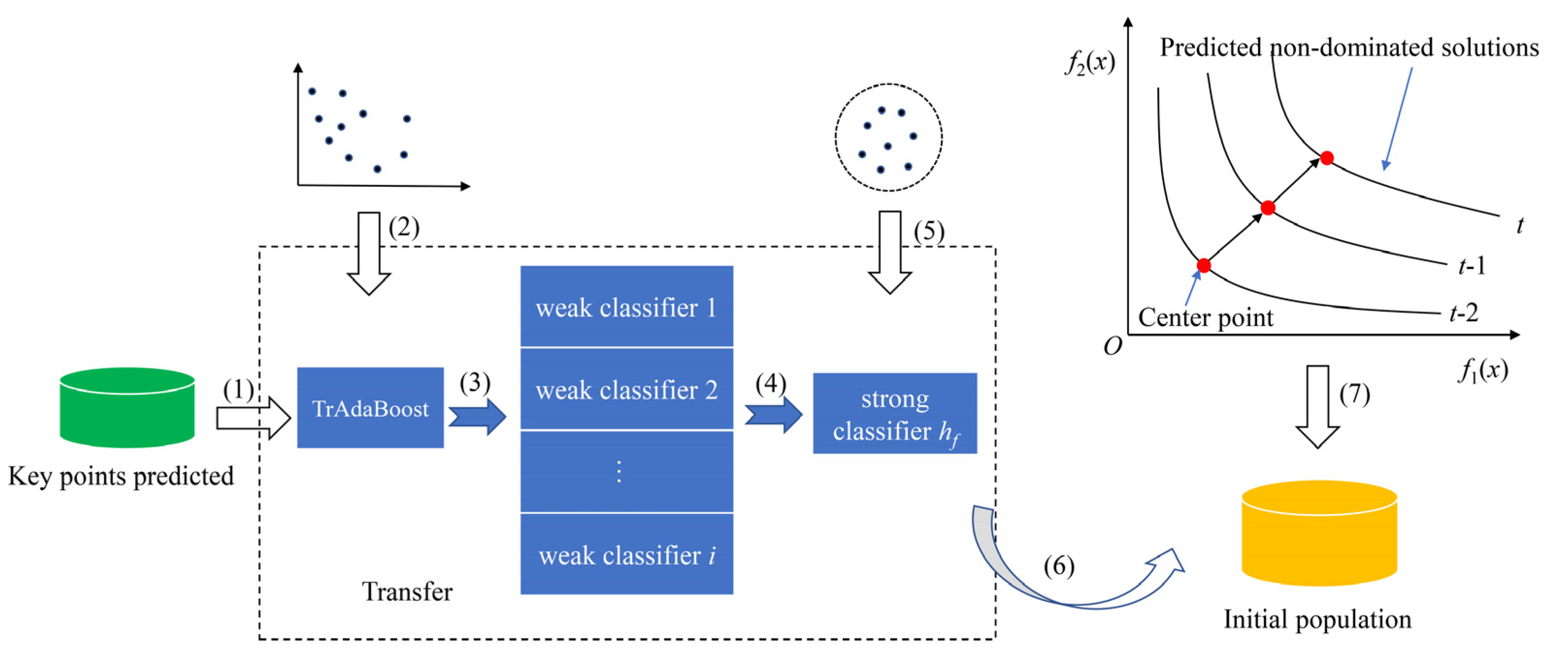
3.4. Transfer

When the key points predicted are generated, the transfer procedure will begin. The main idea of TrAdaBoost is to train a strong classifier h_f by using the obtained key points and the optimal solutions of the previous generation. Once the training process is completed, the classifier h_f can identify the good individuals among the randomly generated individuals as the predicted individuals. During the transfer procedure, the key points obtained above are regarded as the target domain X_ta, and the Pareto-optimal solutions of the previous generation are considered as the source domain X_so.

The basic learning algorithm TrAdaBoost continuously adjusts the weights and parameters of the weak classifiers h_q and then merges the weak classifiers with different weights into strong classifiers. During this period, if an individual in the target domain is misclassified by h_q, its weight value should be increased, indicating that it is critical in the subsequent training. On the other hand, if an individual in the source domain is misclassified by h_q, its weight value should be diminished, suggesting that it is more different from the individuals in the target domain.

Algorithm 4: Transfer (TF)

Input: Pareto-optimal set POSt−1 at the moment t − 1, predicted key points PreKPointst at moment t.

Output: Transferred individuals TransSol.

Xta = PreKPointst;

Xso = POSt−1 $\cup$ Pt−1;

Initialize the weight vector w1(x) = $\frac{1}{\left|X_{so}\right|}$ when x$\in$Xso, w1(x) = $\frac{1}{\left|X_{ta}\right|}$ when x$\in$Xta;

Set a based classifier TrAdaBoost and the number of iterations Qmax;

for i = 1 to Qmax do

Use TrAdaBoost to train a weak classifier $h_q^i$ with data Xso $\cup$ Xta;

Calculate β according to Formula (14);

Calculate βi according to Formula (15);

Update the weights according to Formula (16);

end

Get the strong classifier hf by synthesizing Qmax weak classifiers according to Formula (17);

Randomly generate a large number of solutions xtest;

return TransSol = {x|hf(x)=+1, x$\in$xtest};

The weight update process is as follows. To begin with, we calculate the error rate ε_i of h_q on the target domain X_ta at the ith iteration based on Formula (13).

$${\epsilon }_i={\displaystyle \sum _{x\in X_{ta}}\frac{w_i(x)·|h_q^i(x)-c(x)|}{{\displaystyle {\sum }_{x\in X_{ta}}{w}_i(x)}}}$$

(13)

Then, the coefficients β and β_i of h_q are calculated as:

$$\beta =\frac{1}{2}\ln (\frac{1}{1+\sqrt{2\ln Q_{\max }}})$$

(14)

$${\beta }_i=\frac{1}{2}\ln \frac{1-{\epsilon }_i}{{\epsilon }_i}$$

(15)

Lastly, we update the new weight vectors.

$$w_{i+1}(x)=\{\begin{array}{l}{w}_i(x)·e^{\beta ·|h_q^i(x)-c(x)|},x\in X_{so}\\ w_i(x)·e^{{\beta }_i·|h_q^i(x)-c(x)|},x\in X_{ta}\end{array}$$

(16)

After several iterations, the weight values of individuals that are similar to those in the target domain are increased, and the classification ability of the weak classifier is gradually enhanced. When the iterations are completed, we construct the strong classifier h_f using the following approach.

$$h_f(x)=sign\left({\displaystyle \sum _{i=1}^{Q_{\max }}{\beta }_i{h}_q^i}(x)\right)$$

(17)

Obtaining h_f, we randomly generate many solutions as the training data set x_test, which are put into h_f to classify. Those individuals identified as “good” by h_f will form transferred individuals TransSol. The detailed transfer algorithm procedure can be referred to Algorithm 4.

3.5. Center-Point-Based Feed-Forward Prediction

Diversity maintenance strategies of populations are critical in dynamic evolution. By transferring the excellent individuals of the previous generation, we acquire part of the key points that can be used for evolution while reflecting the overall population status. However, considering the diversity of the whole population, we adopt a feed-forward prediction of the center point to complement the transfer process. Consequently, the initial population is composed of individuals predicted by transfer and individuals generated with the aid of feed-forward prediction model. The specific procedure is shown in Figure 4.

It is well recognized that most people use feed-forward prediction to obtain the entire population, which obviously yields many worthless individuals. Therefore, we only use feed-forward prediction methods to predict non-dominated individuals. We first extract the center points Centers_t−1 and Centers_t−2 from the key points KPoints_t−1 and KPoints_t−2 at moments t − 1 and t − 2, respectively, and then calculate the set of non-dominated solution APOS_t at moment t using the following equation:

$$APO{S}_t=PO{S}_{t-1}+Center{s}_{t-1}-Center{s}_{t-2}+Gauss(0,d)$$

(18)

where Gauss(0, d) refers to a Gaussian noise with mean 0 and standard deviation d.

Algorithm 5: Center-point-based feed-forward prediction (CPFF)

Input: Pareto-optimal set POSt−1 at the moment t − 1, key points KPointst−1 and KPointst−2.

Output: Predicted individuals FeeforSol.

Obtain the center points Centerst−1 and Centerst−2 from KPointst−1 and KPointst−2, respectively;

Calculate predicted individuals APOSt according to Formula (18);

Adjust value of APOSt to the predefined range;

return FeeforSol = APOSt;

3.6. Computational Complexity Analysis

This section analyses the computational complexity of KPTHP at one iteration. The major calculation of KPTHP originates from the following aspects according to Algorithm 1. (1) The complexity of the DKP process mainly lies in finding the polar point using TOPSIS method. Calculating TOPSIS score requires O(N) computation, and determining the positive ideal point and negative ideal point requires O(MN) computation, where N is population size and M is the objective number. (2) The complexity of the KPP is derived from calculation of the predicted key points, and the computational complexity is O(k²), where k is number of key points and k is much smaller than N. (3) The TF of KPTHP follows the computational complexities of weak classifiers. In this paper, we refer to TrAdaBoost as a weak classifier, which requires O(N²n), where n is the dimension of decision variables. (4) The computational complexity of CPFF process is O(d²), where d is the total amount of non-dominated individuals. In summary, the computational complexity of the KPTHP in this work is O(N²n).

The computational complexities of the compared algorithms IT-DMOEA, MMTL-DMOEA, KDMOP, and KT-DMOEA are O(N²nI), O(M³n), O(N²M), and O(N²n) according to the settings of the original papers, and I is the number of iterations for individual’s transfer. It can be clearly seen that the computational complexity of KPTHP is similar to KDMOP and KT-DMOEA but lower than IT-DMOEA and MMTL-DMOEA. The compared algorithms will be presented in detail in Section 4.3.

4. Experimental Configuration and Results Analysis

In this section, we first focus on some configurations of the experiments used to evaluate how well KPTHP performs, including benchmark problems in

Table 1. Overview of benchmark problems.

Type	Benchmark Problems
Type I	DF2, F8, dMOP3, FDA1, FDA4
Type II	DF1, DF3, DF4, DF5, F5, F6, F7, F9, F10, dMOP2, FDA3

, performance metrics, compared algorithms, and parameter configurations. Then, the experimental results of KPTHP and six other state-of-the-art algorithms on the diverse benchmark problems are presented. The statistic results of MIGD, DMIGD, HVD, and MMS values for all test instances are summarized in

Table 2. Mean and SD of MIGD indicator obtained by seven algorithms for (n_t, τ_t) = (5, 20).

Problems	(nt, τt)	IT-DMOEA	GM-DMOP	PPS	MMTL-DMOEA	KDMOP	KT-DMOEA	KPTHP
DF1	(5, 20)	0.0337(3.83E-03)	0.0291(2.06E-03)	0.1461(5.23E-02)	0.0289(1.66E-03)	0.2413(6.02E-02)	0.0438(6.38E-03)	0.0233(2.00E-04)
DF2	(5, 20)	0.0123(7.75E-04)	0.0100(6.22E-04)	0.0820(2.38E-02)	0.0125(1.60E-03)	0.0908(1.97E-02)	0.0364(3.00E-03)	0.0058(4.54E-04)
DF3	(5, 20)	0.2168(1.10E-02)	0.1871(9.16E-03)	0.2811(6.96E-02)	0.2252(5.02E-03)	0.2045(2.35E-03)	0.2626(1.73E-02)	0.1588(2.35E-03)
DF4	(5, 20)	0.8793(2.16E-02)	0.8507(1.43E-03)	0.9115(6.03E-02)	0.8391(4.20E-03)	0.8511(3.05E-03)	0.8239(1.84E-02)	0.8420(8.46E-04)
DF5	(5, 20)	1.8169(2.46E-02)	1.5632(2.95E-03)	1.8064(7.77E-02)	1.6310(1.46E-02)	1.5898(2.04E-02)	1.5581(6.66E-03)	1.5577(5.19E-03)
F5	(5, 20)	0.7526(9.99E-02)	0.5419(9.67E-02)	3.8339(2.11E+00)	0.5180(5.07E-02)	3.0704(1.34E+00)	1.3215(3.06E-01)	0.3016(3.26E-02)
F6	(5, 20)	0.3225(3.37E-02)	0.2489(3.06E-02)	1.4344(3.81E-01)	0.2903(3.39E-02)	1.2310(5.12E-01)	1.3567(2.34E-01)	0.2241(1.65E-02)
F7	(5, 20)	0.3528(2.79E-02)	0.2943(3.54E-02)	1.6073(3.98E-01)	0.3907(3.68E-02)	3.0611(1.33E+00)	1.4547(1.79E+00)	0.2038(1.54E-03)
F8	(5, 20)	0.3940(1.40E-02)	0.1958(7.04E-03)	0.1366(1.43E-02)	0.1504(2.13E-02)	0.0963(3.26E-03)	0.3507(4.51E-02)	0.2241(7.70E-03)
F9	(5, 20)	0.4470(5.47E-02)	0.4781(3.55E-02)	3.2191(1.79E+00)	0.4238(5.46E-02)	4.1997(1.85E+00)	1.6493(8.15E-01)	0.2792(2.62E-02)
F10	(5, 20)	0.4329(4.00E-02)	0.4374(4.66E-02)	3.3580(2.67E+00)	0.4661(4.66E-02)	2.6114(8.05E-01)	1.0969(2.96E-01)	0.2814(2.81E-02)
dMOP2	(5, 20)	0.0320(1.84E-03)	0.0292(1.03E-03)	0.1471(3.17E-02)	0.0299(1.91E-03)	0.2297(5.06E-02)	0.0467(8.95E-03)	0.0232(1.91E-04)
dMOP3	(5, 20)	0.0136(3.89E-03)	0.0086(8.17E-04)	0.0760(1.10E-02)	0.0123(9.06E-04)	0.1331(4.14E-02)	0.0389(6.23E-03)	0.0035(1.36E-04)
FDA1	(5, 20)	0.0797(3.18E-02)	0.0214(1.59E-03)	0.0958(5.75E-02)	0.0310(3.51E-03)	0.1135(1.13E-01)	0.0835(1.25E-02)	0.0058(1.94E-04)
FDA3	(5, 20)	0.1191(6.10E-03)	0.1211(3.43E-03)	0.1524(2.94E-02)	0.1152(2.84E-03)	0.1175(2.52E-02)	0.0897(2.16E-02)	0.1074(1.65E-03)
FDA4	(5, 20)	0.1267(5.21E-03)	0.0887(2.25E-03)	0.0824(2.37E-03)	0.0805(2.29E-03)	0.0773(2.02E-03)	0.1131(2.14E-03)	0.0733(5.35E-04)

,

Table 3. Mean and SD of HVD indicator obtained by seven algorithms for (n_t, τ_t) = (5, 20).

Problems	(nt, τt)	IT-DMOEA	GM-DMOP	PPS	MMTL-DMOEA	KDMOP	KT-DMOEA	KPTHP
DF1	(5, 20)	0.0324(4.17E-03)	0.0297(2.75E-03)	0.1416(4.06E-02)	0.0254(2.13E-03)	0.2048(2.92E-02)	0.0584(5.20E-03)	0.0195(3.68E-03)
DF2	(5, 20)	0.0161(2.42E-03)	0.0153(1.75E-03)	0.0820(2.05E-02)	0.0168(2.85E-03)	0.0954(1.94E-02)	0.0433(3.69E-03)	0.0121(1.78E-03)
DF3	(5, 20)	0.2184(7.13E-03)	0.1860(5.78E-03)	0.2616(4.05E-02)	0.2119(7.54E-03)	0.2142(0.42E-03)	0.2631(6.64E-03)	0.1750(6.26E-03)
DF4	(5, 20)	0.3582(1.12E-02)	0.3311(4.42E-03)	0.3551(1.83E-02)	0.3376(3.61E-03)	0.3371(2.78E-03)	0.3348(8.81E-03)	0.3271(5.02E-03)
DF5	(5, 20)	0.3518(4.00E-03)	0.3337(4.44E-03)	0.3867(3.02E-02)	0.3497(2.83E-03)	0.3609(1.43E-02)	0.3440(4.29E-03)	0.3320(2.90E-03)
F5	(5, 20)	0.5009(3.70E-02)	0.4060(5.43E-02)	0.6242(2.48E-02)	0.4481(3.87E-02)	0.6849(4.81E-02)	0.6409(3.93E-02)	0.2921(2.11E-02)
F6	(5, 20)	0.2715(1.24E-02)	0.2432(2.47E-02)	0.5647(1.58E-02)	0.2794(2.06E-02)	0.5620(2.95E-02)	0.5940(6.14E-02)	0.2308(1.44E-02)
F7	(5, 20)	0.3061(1.77E-02)	0.2657(2.49E-02)	0.4948(1.40E-02)	0.3432(0.79E-02)	0.4947(4.24E-02)	0.5105(4.60E-02)	0.2060(1.11E-02)
F8	(5, 20)	0.3780(1.69E-02)	0.1522(5.69E-03)	0.0856(1.77E-02)	0.1022(2.36E-02)	0.0536(2.96E-03)	0.1960(2.46E-02)	0.1783(8.10E-03)
F9	(5, 20)	0.3571(2.54E-02)	0.4042(2.25E-02)	0.6780(4.07E-02)	0.3848(3.28E-02)	0.7126(3.72E-02)	0.5997(2.20E-02)	0.2584(1.66E-02)
F10	(5, 20)	0.3588(2.06E-02)	0.3740(2.72E-02)	0.6475(3.17E-02)	0.4036(2.12E-02)	0.6717(4.37E-02)	0.5696(2.86E-02)	0.2563(1.78E-02)
dMOP2	(5, 20)	0.0314(3.75E-03)	0.0299(3.69E-03)	0.1483(2.50E-02)	0.0289(3.47E-03)	0.2008(2.30E-02)	0.0590(9.31E-03)	0.0216(4.30E-03)
dMOP3	(5, 20)	0.0199(3.85E-03)	0.0166(1.87E-03)	0.0772(1.07E-02)	0.0198(3.11E-03)	0.1244(3.24E-02)	0.0474(6.59E-03)	0.0131(1.93E-03)
FDA1	(5, 20)	0.0739(2.34E-02)	0.0274(2.88E-03)	0.0908(4.16E-02)	0.0363(7.83E-03)	0.1004(6.74E-02)	0.0890(1.10E-02)	0.0129(2.61E-03)
FDA3	(5, 20)	0.1237(1.72E-02)	0.1400(7.39E-03)	0.1472(1.80E-02)	0.1118(6.59E-03)	0.1162(9.00E-03)	0.0707(1.16E-02)	0.1148(4.34E-03)
FDA4	(5, 20)	0.0957(8.72E-03)	0.0543(4.00E-03)	0.0483(3.59E-03)	0.0475(3.94E-03)	0.0436(4.21E-03)	0.0725(4.96E-03)	0.0387(3.58E-03)

,

Table 4. Mean and SD of MMS indicator obtained by seven algorithms for (n_t, τ_t) = (5, 20).

Problems	(nt, τt)	IT-DMOEA	GM-DMOP	PPS	MMTL-DMOEA	KDMOP	KT-DMOEA	KPTHP
DF1	(5, 20)	0.9752(3.42E-03)	0.9807(4.72E-03)	0.8840(2.45E-02)	0.9871(4.10E-03)	0.8546(2.52E-02)	0.8849(1.31E-02)	0.9948(6.02E-04)
DF2	(5, 20)	0.9886(1.82E-03)	0.9910(9.37E-04)	0.9128(2.56E-02)	0.9920(1.41E-03	0.9243(2.10E-02)	0.8617(1.15E-02)	0.9950(4.43E-04)
DF3	(5, 20)	0.6789(1.85E-02)	0.7229(8.98E-03)	0.6284(3.76E-02)	0.6988(7.77E-03)	0.6426(6.65E-03)	0.5110(1.44E-02)	0.7459(7.02E-03)
DF4	(5, 20)	0.3601(1.21E-02)	0.3461(1.66E-03)	0.3479(1.51E-02)	0.3569(5.19E-03)	0.3007(6.08E-03)	0.2962(1.36E-02)	0.3451(1.35E-03)
DF5	(5, 20)	0.9978(4.47E-03)	1.0000(1.29E-05)	0.9998(1.39E-04)	1.0000(1.27E-06)	1.0000(2.14E-05)	0.8715(1.49E-02)	1.0000(1.48E-05)
F5	(5, 20)	0.7909(2.21E-02)	0.8388(2.05E-02)	0.5709(0.18E-01)	0.8222(7.21E-03)	0.5960(1.03E-01)	0.3705(4.47E-02)	0.8873(1.26E-02)
F6	(5, 20)	0.8978(1.24E-02)	0.9237(6.89E-03)	0.7536(5.06E-02)	0.8873(0.60E-03)	0.7297(3.57E-02)	0.3937(5.72E-02)	0.9144(4.69E-03)
F7	(5, 20)	0.8866(2.00E-02)	0.8959(1.40E-02)	0.7105(6.80E-02)	0.8685(1.35E-02)	0.6955(4.80E-02)	0.3735(0.64E-02)	0.9167(6.34E-03)
F8	(5, 20)	0.9995(1.13E-03)	1.0000(1.74E-05)	1.0000(2.15E-06)	1.0000(8.10E-07)	1.0000(2.37E-06)	0.9362(2.18E-02)	1.0000(4.64E-06)
F9	(5, 20)	0.8745(1.68E-02)	0.8481(1.02E-02)	0.5440(9.17E-02)	0.8662(7.50E-03)	0.6212(6.63E-02)	0.3389(4.85E-02)	0.9011(8.28E-03)
F10	(5, 20)	0.8748(1.61E-02)	0.8624(1.38E-02)	0.6443(0.32E-01)	0.8782(1.09E-02)	0.7309(7.58E-02)	0.3560(6.69E-02)	0.9006(1.05E-02)
dMOP2	(5, 20)	0.9757(2.45E-03)	0.9814(2.40E-03)	0.8764(2.15E-02)	0.9845(3.25E-03)	0.8598(2.32E-02)	0.8897(2.01E-02)	0.9945(6.98E-04)
dMOP3	(5, 20)	0.9870(7.28E-03)	0.9917(7.82E-04)	0.9452(9.47E-03)	0.9919(2.07E-03)	0.9165(2.17E-02)	0.8456(2.72E-02)	0.9967(5.69E-04)
FDA1	(5, 20)	0.7755(3.24E-02)	0.9057(1.42E-02)	0.7094(8.69E-02)	0.8960(2.58E-02)	0.6599(5.07E-02)	0.7234(3.78E-02)	0.9575(5.38E-03)
FDA3	(5, 20)	0.7563(2.59E-02)	0.7917(2.56E-02)	0.5050(6.65E-02)	0.8179(5.28E-02)	0.7132(8.60E-02)	0.7960(5.70E-02)	0.9035(1.32E-02)
FDA4	(5, 20)	0.9996(6.67E-05)	0.9999(2.51E-05)	1.0000 (2.13E-05)	1.0000(2.55E-05)	1.0000(1.37E-05)	0.9965(1.56E-03)	1.0000(1.09E-05)

and

Table 5. DMIGD values obtained by seven algorithms.

Problems	IT-DMOEA	GM-DMOP	PPS	MMTL-DMOEA	KDMOP	KT-DMOEA	KPTHP
DF1	0.1208	0.1001	0.8777	0.1042	0.6352	0.1337	0.0461
DF2	0.0680	0.0679	0.5504	0.0745	0.3599	0.1049	0.0435
DF3	0.3599	0.2840	0.6749	0.3353	0.7743	0.3891	0.2433
DF4	1.2602	1.0558	1.9254	0.9836	1.1612	1.0198	0.9916
DF5	1.7444	1.4376	1.9952	1.5013	1.9323	1.3356	1.3186
F5	2.2424	1.9243	64.5888	2.1040	14.6895	2.4746	1.4258
F6	1.2605	1.0831	5.1151	1.0915	11.1875	2.2036	0.9947
F7	1.3042	1.2183	5.3431	1.3596	15.5639	2.0192	0.9524
F8	0.8473	0.4427	0.4336	0.3495	0.1885	0.3960	0.4709
F9	1.2984	1.4424	18.1299	1.4344	9.0901	1.8461	1.0744
F10	1.5885	1.7056	18.1954	1.7896	6.0834	1.8939	1.5591
dMOP2	0.0855	0.0738	0.6389	0.0979	0.4667	0.0890	0.0440
dMOP3	0.0477	0.0430	0.4178	0.0676	0.3104	0.0759	0.0190
FDA1	0.2684	0.1231	0.8779	0.1849	1.1173	0.1626	0.0814
FDA3	0.2277	0.1681	0.4224	0.1802	0.2239	0.1262	0.1213
FDA4	0.2555	0.1768	0.1966	0.1404	0.1552	0.1352	0.1104

, respectively. In particular, the values with the best results have a darker color. For the sake of fairness, the change frequency τ_t and change severity n_t are fixed to 5 and 20 among all algorithms in this section of the experiment. All experimental procedures are performed under the same hardware configuration, all in MATLAB R2020b.

4.1. Benchmark Problems

To solve DMOPs, the proposed KPTHP is tested on sixteen test problems, including five DF problems [66], six F problems [34], two dMOP problems [27,67], and three FDA problems [27,67,68]. The attributes and characteristics of the benchmark problems are described in Table 1. The POFs of these test functions considered have different characteristics, including linear and nonlinear, continuous and discontinuous, and convex and concave.

In the test suite DF, POF and POS are dynamic, and DF2 has severe diversity loss. The problems F5–F8 have nonlinear correlation between decision variables. In F9, POF jumps from one scope to another scope occasionally, and in F10, the geometric shapes of two consecutive POFs are totally different from each other. In the test suite FDA, the POF and/or POS vary over time, while the number of decision variables, the number of targets, and the boundaries of the search space remain fixed. The dMOP problems are the extensions of FDA problems. Among all the tested functions, F8 and FDA4 refer to three-objective functions, while the remaining functions are two-objective ones. The time instance t is defined as $t=\frac{1}{n_t}\lfloor \frac{\tau }{{\tau }_t}\rfloor$, where n_t, τ, and τ_t represent the severity of change, maximum number of iterations, and the frequency of change, respectively.

4.2. Performance Metrics

Performance metrics play an important role in assessing the performance of algorithms in different aspects. In our experimental study, four metrics were adopted, including modified inverted generational distance (MIGD), DMIGD, modified maximum spread (MMS), and hypervolume difference (HVD).

4.2.1. MIGD

IGD [32,34,69] is a widely adopted metric to evaluate the convergence and diversity of multi-objective evolutionary algorithms. It represents the shortest distance between the true POF and the POF obtained by the evolutionary algorithm. The calculation formula is as follows:

$$IGD(P{F}_t^{*},P{F}_t)=\frac{{\displaystyle \sum _{x\in P{F}_t^{*}}{min}_{x\in P{F}_t}\left|\right|x^{*}-x\left|\right|}}{\left|P{F}_t^{*}\right|}$$

(19)

where $P{F}_t^{*}$ and $P{F}_t$ denote the true Pareto front and the approximate Pareto front obtained by the algorithm at the moment t, respectively, and $\left|P{F}_t^{*}\right|$ indicates the individual number of true POF. The smaller the IGD value, the better the convergence and diversity of the obtained solutions.

On the basis of IGD, we calculate the average IGD value for the whole environment change as MIGD:

$$MIGD=\frac{1}{\left|T\right|}{\displaystyle \sum _{t\in T}IGD(P{F}_t^{*},P{F}_t)}$$

(20)

where T is the number of environment changes in one run and |T| is the cardinality of T.

4.2.2. DMIGD

DMIGD [56] is used to evaluate the overall performance of each benchmark function at different change frequencies and severities, where it is expected that the smaller, the better:

$$DMIGD=\frac{1}{\left|E\right|}{\displaystyle \sum _{c\in E}MIGD(C)}$$

(21)

where C represents different environment configurations and E denotes all the environmental conditions.

4.2.3. MMS

MMS [70,71] is used to measure the mean ability of the acquired solution to cover the true POF. A larger MMS indicates wider coverage of the obtained solutions. MMS is defined as:

$$MMS(P{F}_t^{*},PF)=\frac{1}{\left|T\right|}{\displaystyle \sum _{t\in T}MS(P{F}_t^{*},P{F}_t)}$$

(22)

$$MS(P{F}^{*},PF)=\sqrt{\frac{1}{M}{{\displaystyle \sum _{k=1}^M\left[\frac{min\left[P{F}_k^{*max},P{F}_k^{max}\right]-max\left[P{F}_k^{*min},P{F}_k^{min}\right]}{P{F}_k^{*max}-P{F}_k^{*min}}\right]}}^2}$$

(23)

where $P{F}_k^{*max}$ and $P{F}_k^{*min}$ denote the maximum and minimum of the kth objective in true POF, respectively; $P{F}_k^{max}$ and $P{F}_k^{min}$ denote the maximum and minimum of the kth objective in the obtained POF, respectively.

4.2.4. HVD

HVD [72,73,74] represents the hypervolume difference between $P{F}_t^{*}$ and $P{F}_t$ and is computed as:

$$HVD(P{F}_t^{*},P{F}_t)=HV(P{F}_t^{*})-HV(P{F}_t)$$

(24)

where HV(PF) represents the hypervolume of POF. A smaller HVD indicates better convergence and diversity performance of the algorithm.

4.3. Comparison Algorithms and Parameter Settings

Six state-of-the-art dynamic multi-objective evolutionary algorithms are identified for the purpose of comparison with KPTHP, including PPS, GM-DMOP, MMTL-DMOEA, IT-DMOEA, KT-DMOEA, and KDMOP. Meanwhile, an introduction of each algorithm and the related parameter configuration will be presented as follows.

(1)

PPS [34]: Zhou et al. proposed a dynamic multi-objective evolutionary algorithm based on population prediction strategy (PPS), where a Pareto set is divided into two parts: a center point and a manifold. The individuals of the population at the next moment consist of the predicted center point and estimated manifold together. This method has an excellent performance in dealing with linear or nonlinear correlation between design variables.

(2)

GM-DMOP [37]: Wang et al. introduced a grey prediction model into dynamic multi-objective optimization for the first time. The basic idea of GM-DMOP is that the centroid point at the next moment is predicted by a grey prediction model when detecting the environmental changes. One of the highlights of the algorithm is dividing the population into clusters and predicting the centroid points of each cluster to increase the accuracy of the prediction. It has been proven that the grey prediction method brings excellent population convergence and diversity.

(3)

MMTL-DMOEA [71]: MMTL-DMOEA is a new memory-driven manifold transfer-based evolutionary algorithm for dynamic multi-objective optimization. The initial population is composed of the elite individuals obtained from both experience and future prediction. The approach is capable of improving the computational speed while acquiring a better quality of solutions.

(4)

IT-DMOEA [70]: Jiang et al. designed an individual transfer-based algorithm, where a presearch strategy is used for filtering out some high-quality individuals with better diversity. The merit of IT-DMOEA is that it maintains the advantages of transfer learning methods and reduces the occurrence of negative transfer.

(5)

KT-DMOEA [75]: KT-DMOEA adopted a method based on a trend prediction model and imbalance transfer learning to effectively track the moving POF or POS. It integrates a small number of high-quality individuals with the imbalance transfer learning technique seamlessly, greatly improving the performance of dynamic optimization.

(6)

KDMOP [64]: KDMOP was proposed recently by Yen et al., and it introduces a well-regarded multi-attribute decision-making strategy called TOPSIS. TOPSIS is utilized to obtain the initial population in a new environment, and it is used to select good individuals in mating selection and environmental selection.

The relevant experimental parameters are set as follows. For all algorithms, the population size is set to 100 for bi-objective optimization problems and 200 for tri-objective optimization, and the dimension of decision variables is set according to [66,67,68]. All the problems are run 30 times independently on benchmark problems, and the environmental changes are set to 20 times in each run. For a fair comparison, the specific parameters for PPS, GM-DMOP, MMTL-DMOEA, IT-DMOEA, KT-DMOEA, and KDMOP are set according to their original publications [34,37,64,70,71,75]. For KPTHP, in the transfer stage, most of the parameters in the TrAdaBoost are set by default [76]. The typical static multi-objective optimizers contain RM-MEDA [77], NSGA-II [78], MOEA/D [79], etc. In this paper, we choose RM-MEDA as the SMOEA optimizer.

4.4. Results on DF and F Problems

Table 2 shows the MIGD values obtained by the seven algorithms. KPTHP has the smallest MIGD values for the eleven DF and F test functions, while KDMOP and KT-DMOEA have the smallest MIGD values only in F8 and DF4, respectively. The distribution of the algorithms obtaining the second-best value is more fragmented. KPTHP may be more advantageous while dealing with problems where there is a nonlinear correlation between decision variables. For F9 and F10, their Pareto sets occasionally jump from one area to another, or the geometry of consecutive POFs is completely different, yet KPTHP obviously performs better and more competitively compared with the other algorithms.

The statistical results of the HVD metrics for the seven algorithms are presented in Table 3. We can clearly observe that the distribution of MIGD values and HVD values for the well-performing test functions is almost the same. The only difference is that KPTHP obtains the best HVD value instead of KT-DMOEA in DF4. There are two main explanations. The first is that one of the characteristics of DF4 is its dynamically changing boundary values, and the second is that KPTHP pays more attention to the boundary points in evaluating the performance of the algorithm, while KT-DMOEA mainly focuses on the effect of knee points and pays little attention to boundary points.

Table 4 shows the MS values and standard deviations of the seven algorithms. It is obvious that KPTHP has a better performance than the other six comparison algorithms on many of the tested functions. MMTL-DMOEA performs best on the two test functions, followed by GM-DMOP and IT-DMOEA gaining one best result each. The above experimental results demonstrate that KPTHP can obtain a great many individuals with excellent convergence and diversity. For DF5 and F8, on which the results are not the best, however, KPTHP is remarkably similar in performance to MMTL-DMOEA with the best results.

4.5. Results on FDA and dMOP Problems

The FDA and dMOP test functions are linearly linked between the decision variables. For the MIGD, HVD, and MMS values in Table 2, Table 3, and Table 4, it can be observed that KPTHP has a better performance than the other six algorithms in many of the tested functions, and especially in MMS indicator is completely superior to them. In the remaining six algorithms, PPS utilizes substantial prime points to train the AR model, but in effect, there are simply not enough high-quality prime points to support accurate predictions at this early stage of evolution, rendering performance incompetent. IT-DMOEA, MMTL-DMOEA, and KT-DMOEA are based on transfer learning methods. Although they reduce the occurrence of negative transfer to some extent, the quality of transferred individuals is inferior to KPTHP. KDMOP mainly predicts individuals depending on the direction of point evolution, and consequently, there is not much superiority in the test functions where POF changes frequently. The performance of the algorithms is further analyzed as follows according to the characteristics of the test functions.

The POFs of dMOP2, FDA1, and FDA4 all vary in a sinusoidal pattern with periodic and symmetric variation. It can be inferred that the three test functions have similar variations. The values of MIGD, HVD, and MMS of KPTHP are extremely outstanding compared to other algorithms. Therefore, KPTHP combining key-points-based transfer learning and hybrid prediction strategies can predict more accurately the individuals at the next moment and has a significantly better performance on the three test functions. The POFs of both dMOP3 and FDA4 are constant. According to the three indicators, it can be introduced that KPTHP may be also very effective in solving the test functions that have static POF during the change. It is worth mentioning that FDA4 is a test function of the three objectives. Based on the MMS values, KPTHP can acquire better diversity in solving the triple-objective function.

4.6. Results on DMIGD Metric

In total, we performed experimental comparisons on five pairs of parameters of n_t and τ_t, including (5, 5), (5, 10), (5, 15), (5, 20), and (10, 5). Table 5 shows the DMIGD values for each algorithm on all tested functions. KPTHP obtained the best values on fourteen test functions, followed by MMTL-DMOEA and KDMOP on only one test function each, DF4 and F8, respectively. It can be straightforward to deduce that KPTHP can obtain good convergence performance and maintain great diversity. The excellent assignment of DMIGD values to the test functions is very similar to the MIGD values, which indicates that KPTHP is excellent not only in terms of single parameter configuration but also in terms of overall performance.

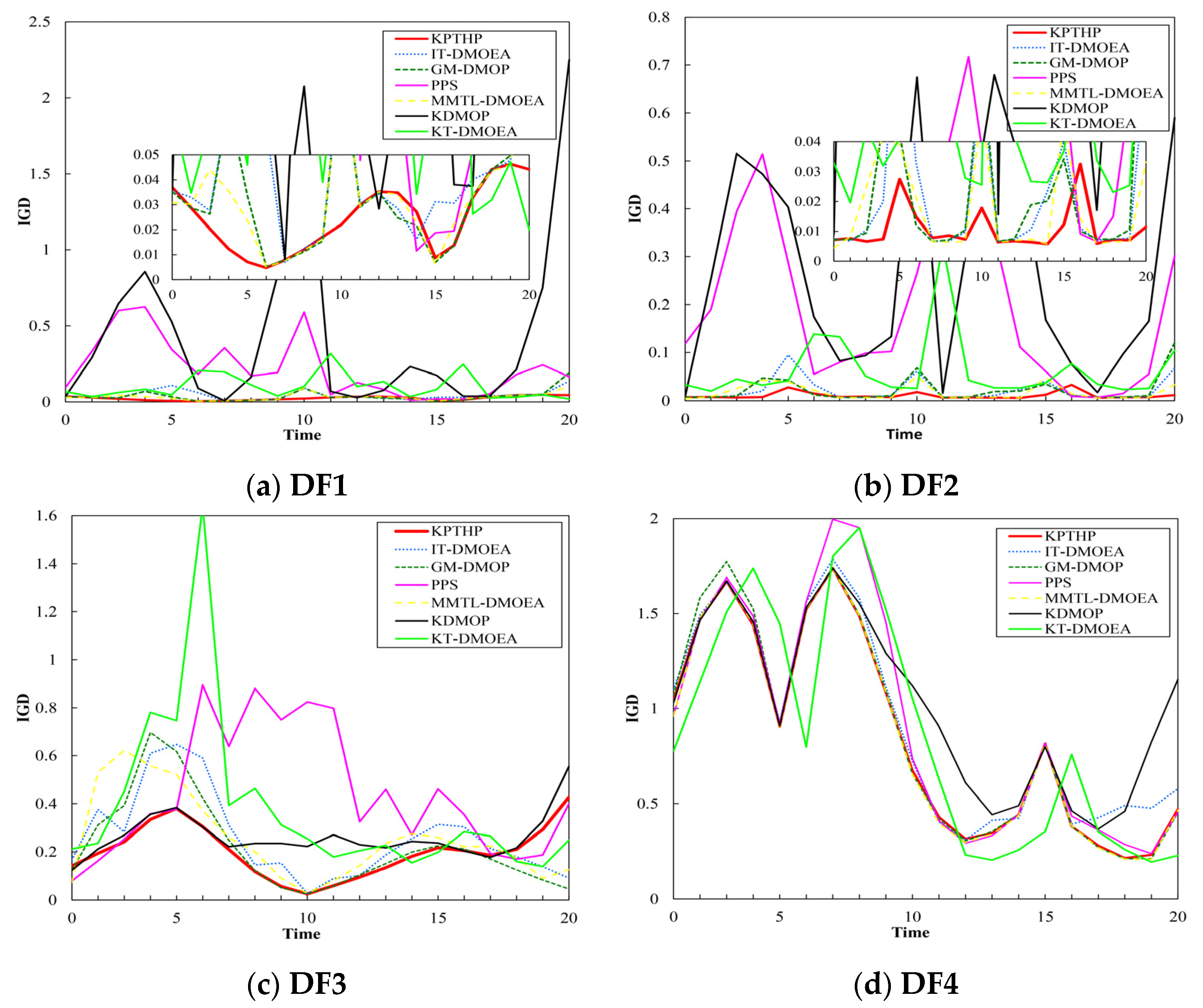
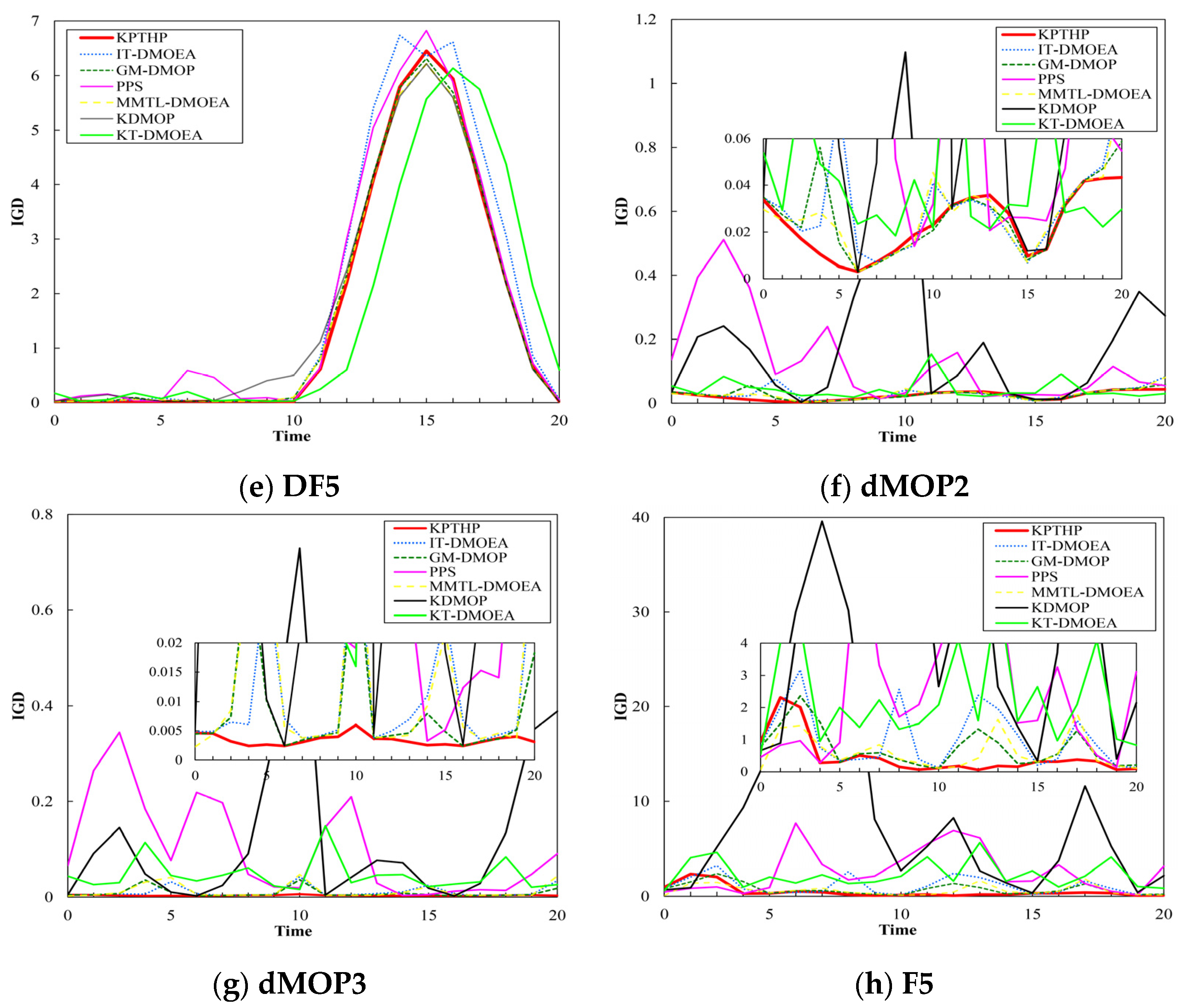
4.7. Analyzing the Evolutionary Processes of the Compared Algorithms

Above, we analyzed the performance of the algorithm running on the test functions under the four metrics. In the following, we present a visualization of the excellent performance of the algorithm, including the IGD evolution curves of the sixteen functions at different moments and the POFs of FDA1, dMOP2, and DF2 obtained by the seven algorithms. The change frequency τ_t and change severity n_t of all the algorithms are fixed to (5, 20).

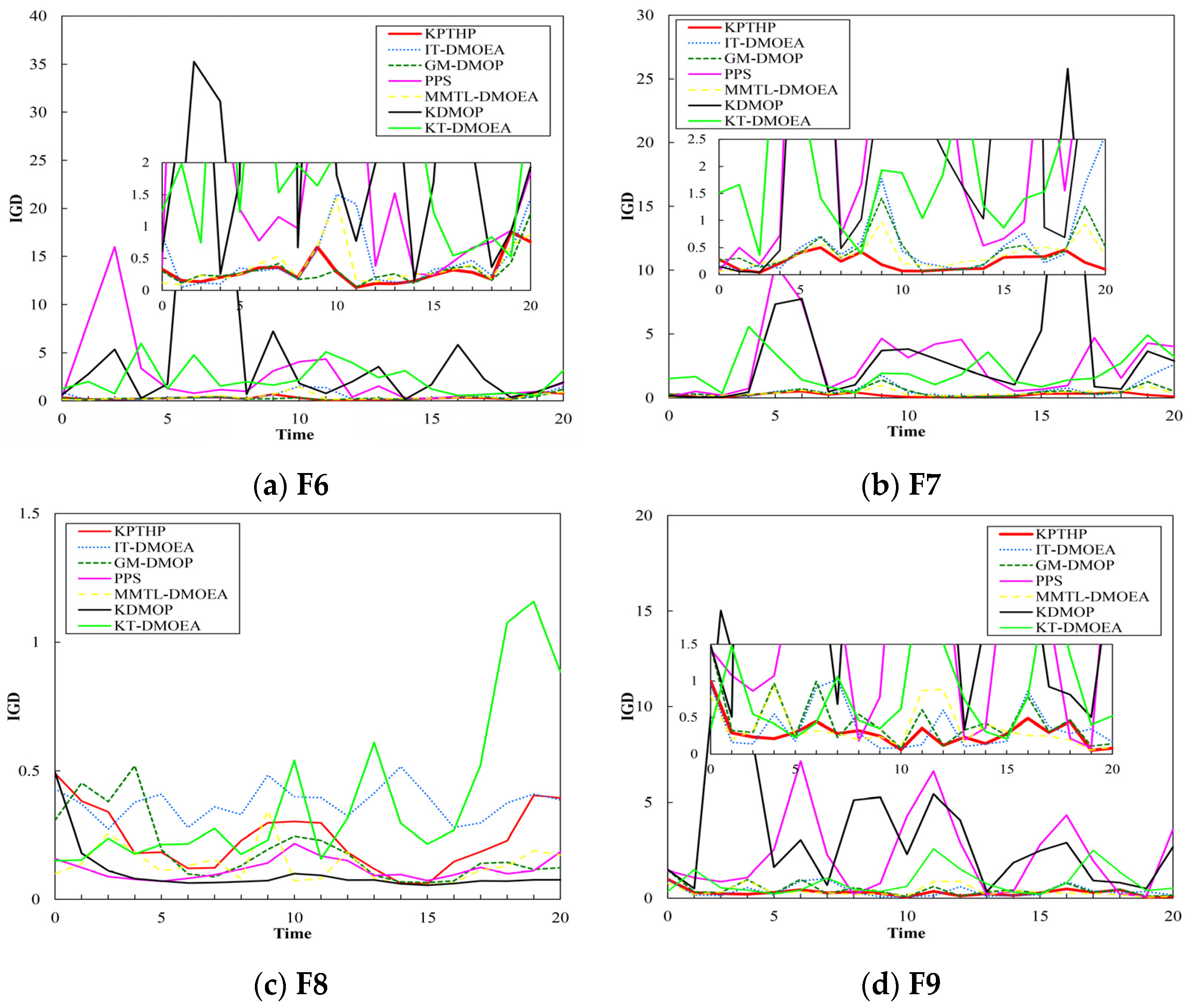
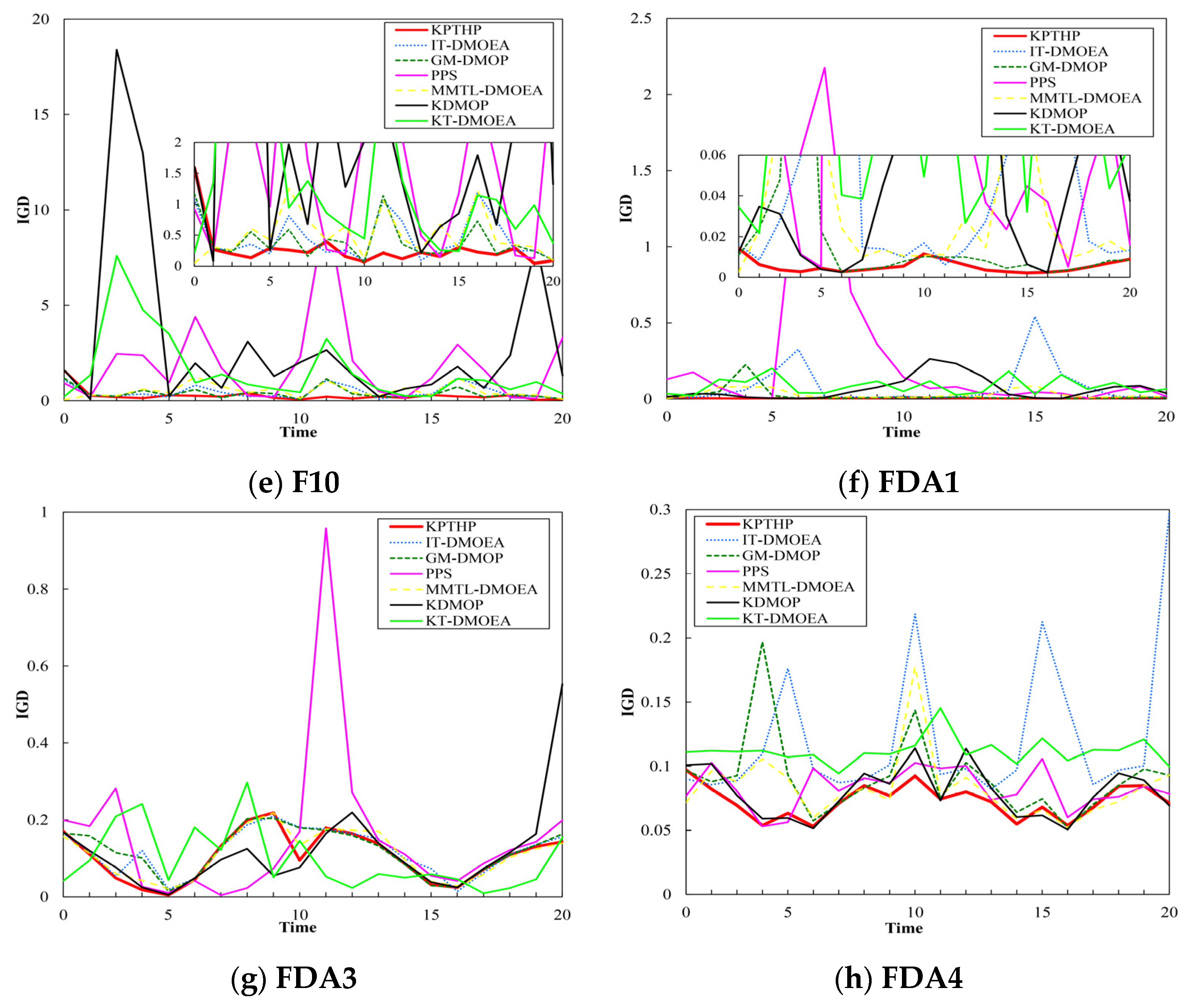
Figure 5 and Figure 6 show the IGD variation curves for all the tested functions. It can be visually observed that KPTHP has outstanding performance in most of the tested functions, which indicates that KPTHP is more able to cope with the effects of environmental changes. From the figures, we can see that KDMOP often has IGD peaks in some test problems, such as dMOP2, dMOP3, F6, and F10, which indicates the instability of this algorithm in the evolutionary process. The possible reasons for this occurrence are the drastic nature of POF change and the nonlinear correlation, which can cause errors in the predicted direction. On FDA4 and F8, IT-DMOEA does not perform satisfactorily, probably because the guided population based on the reference vector does not behave well in three-objective problems.

What can be clearly noticed is that KT-DMOP fluctuates more significantly in most of the tested functions, especially DF3 and F8, which may indicate a lack of predictive accuracy capability of the algorithm in the case of irregular knee points. However, KPTHP maintains stable variation in the vast majority of cases, except for DF4 and DF5. An important reason for this is that the transfer based on key points predicted is able to predict the adequate key points at the next moment with a large degree of accuracy, avoiding large deviations from the true POF. Another essential reason is that the center-point-based feed-forward prediction can directly predict non-dominated solutions at the next moment, which plays an important complementary role to the transfer procedure. Although this method alone is inefficient and has poor accuracy in mixed convexity–concavity or POFs with strong variations, it can provide a partially high-quality prediction of individuals to some extent regardless of whether the POFs vary linearly or non-linearly.

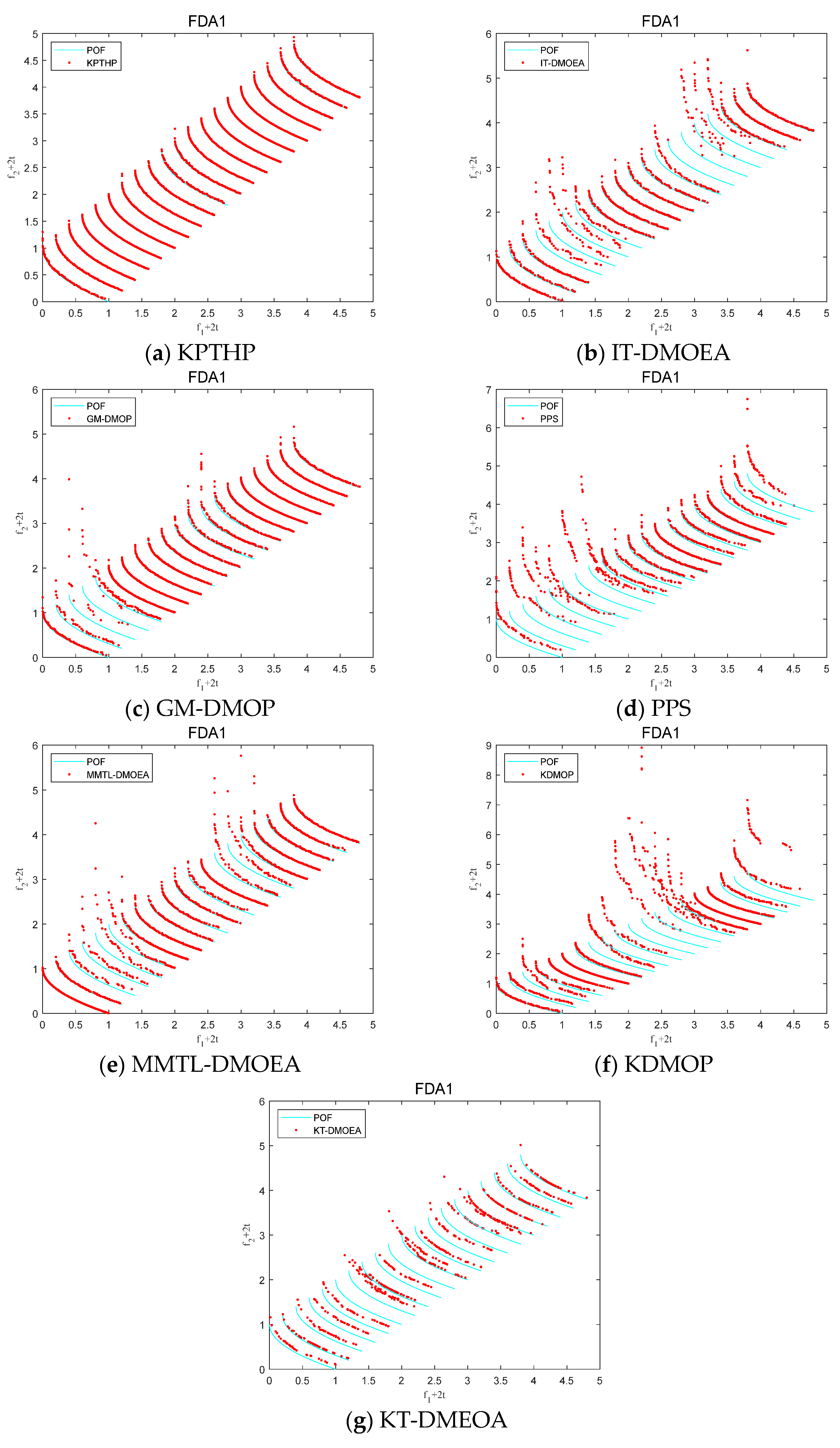
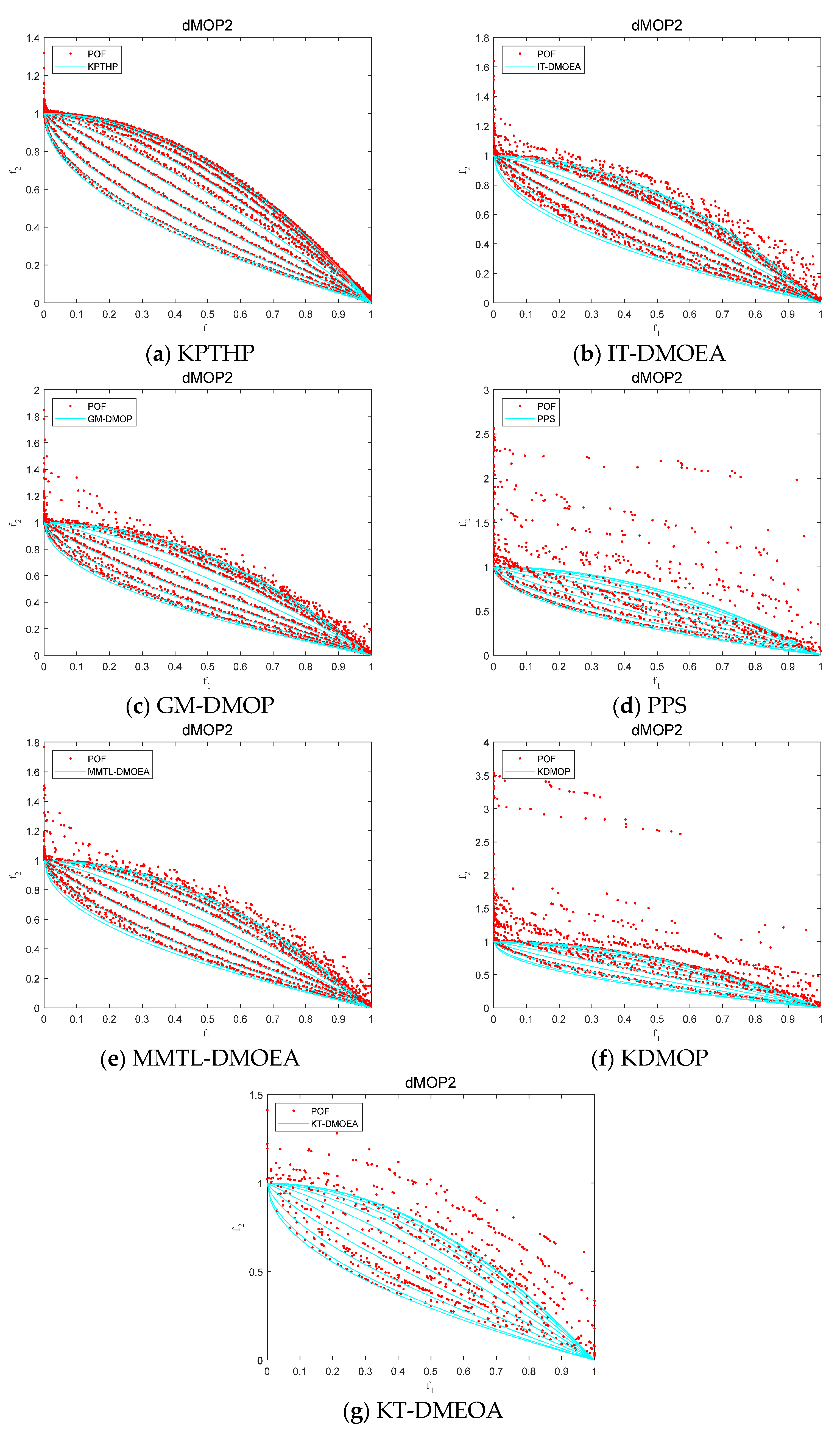
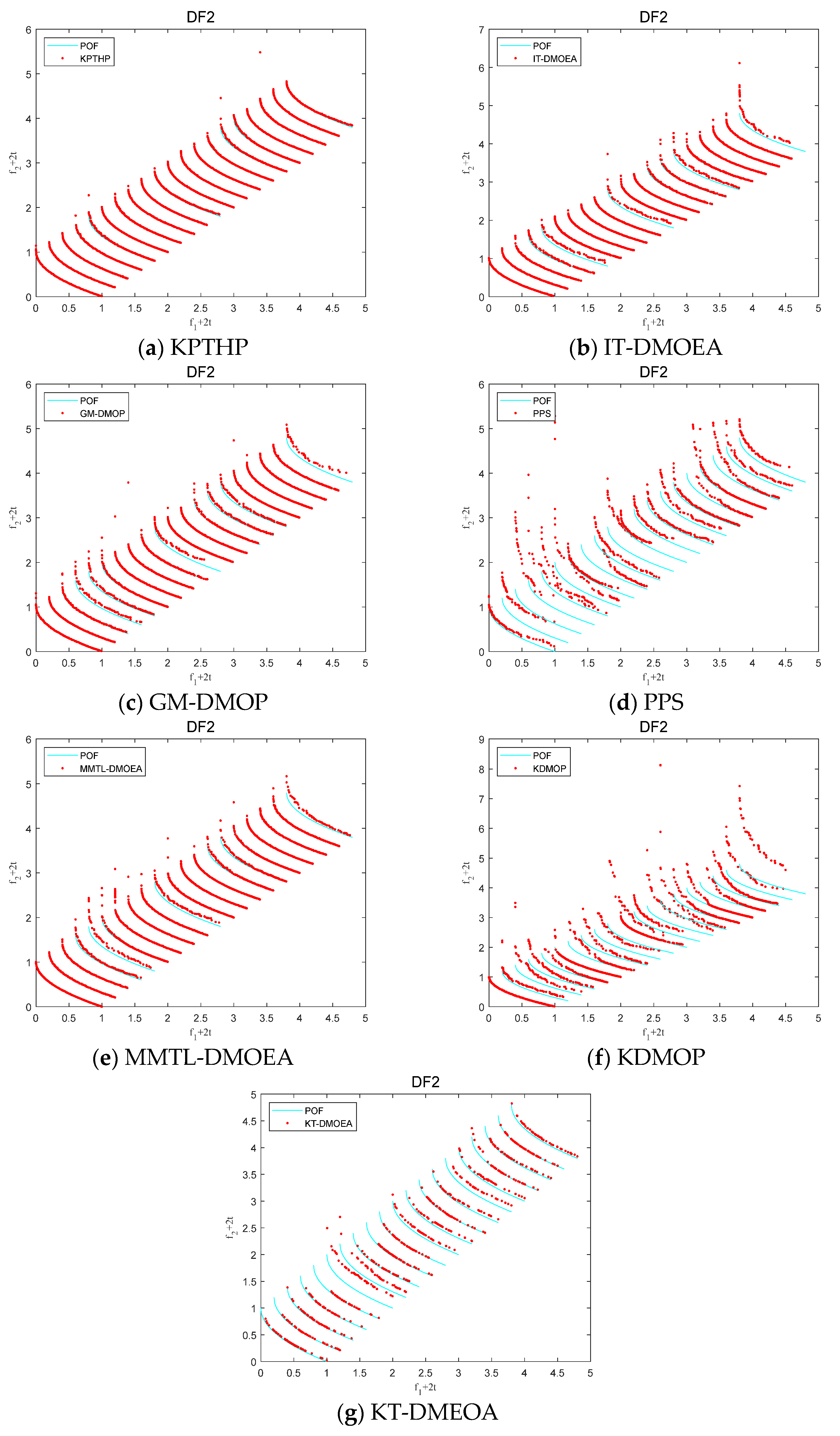
Figure 7, Figure 8 and Figure 9 show the true POF and the actual solution set by FDA, dMOP2, and DF2 at thirty different moments. Meanwhile, the actual solution set is marked with red dots, and the true POF is marked with blue curves. It can be clearly seen that KPTHP maintains good convergence and diversity at different moments. For DFA1 and DF2, the ability of PPS, KDMOP, and KT-DMOEA to track the true POF is very poor most of the time, and the approximate Pareto front acquired deviates from the true POF very seriously. Because the core idea of both PPS and KDMOP is center-point-based prediction solely, the evolutionary direction determined by the center point is not effective when the true POF is unchanged. KT-DMOEA is a knee-points-based prediction method, which is mainly focused on the movement of knee points and has great limitation and instability. For dMOP2, it is obvious that the distribution of population individuals for the six algorithms compared is very uneven.

For IT-DMOEA, because the evolution of the population relies on the role of the reference vector, the capability of generating the guided population decreases in the case of concave and convex changes of POF, while KPTHP can maintain a very good distribution, probably benefiting from two factors. One is that the key points are a microcosm of the true POF, which are small in number. However, we can generate many reliable and similarly distributed individuals through the action of transfer learning. The second is that for the case of relatively regular changes in the true POF, the center-point-based prediction can complement the key-points-based transfer process, thus combining each other’s excellent features perfectly.

5. Further Discussion

5.1. Influence of Change Frequency

This section mainly explores the effect of change frequency on seven different algorithms. The experiments are still performed on DF, F, dMOP, and FDA test functions. Furthermore, n_t is set to 5 fixedly, and τ_t is set to 10, 15, and 20 successively. The experimental performance of different algorithms on MIGD and HVD is shown in

Table 6. Mean and SD of MIGD indicator obtained by seven algorithms for (n_t, τ_t) = (5, 10), (5, 15), and (5, 20).

Problems	(nt, τt)	IT-DMOEA	GM-DMOP	PPS	MMTL-DMOEA	KDMOP	KT-DMOEA	KPTHP
DF1	(5, 10)	0.0742(8.59E-03)	0.0645(3.66E-03)	0.6153(2.55E-01)	0.0861(7.89E-03)	0.5213(5.88E-02)	0.0845(9.50E-03)	0.0294(4.97E-04)
	(5, 15)	0.0616(2.60E-03)	0.0574(3.70E-03)	0.8661(3.27E-01)	0.0473(1.18E-03)	0.5536(3.38E-02)	0.1160(3.51E-02)	0.0256(1.00E-04)
	(5, 20)	0.0337(3.83E-03)	0.0291(2.06E-03)	0.1461(0.23E-02)	0.0289(1.66E-03)	0.2413(6.02E-02)	0.0438(6.38E-03)	0.0233(0.00E-04)
DF2	(5, 10)	0.0418(5.57E-03)	0.0484(3.84E-03)	0.3260(7.98E-02)	0.0582(5.62E-03)	0.2263(5.24E-02)	0.0765(1.04E-02)	0.0276(9.93E-04)
	(5, 15)	0.0359(3.08E-03)	0.0361(4.95E-03)	0.3416(1.39E-01)	0.0284(5.26E-03)	0.3076(6.30E-02)	0.0613(7.42E-03)	0.0159(1.13E-03)
	(5, 20)	0.0123(7.75E-04)	0.0100(6.22E-04)	0.0820(2.38E-02)	0.0125(1.60E-03)	0.0908(1.97E-02)	0.0364(3.00E-03)	0.0058(4.54E-04)
DF3	(5, 10)	0.3141(1.31E-02)	0.2344(1.22E-02)	0.3724(7.64E-02)	0.3076(2.51E-02)	0.2604(5.31E-02)	0.3212(9.95E-02)	0.2003(1.13E-02)
	(5, 15)	0.3033(6.40E-03)	0.2312(1.15E-02)	0.4433(1.58E-01)	0.2739(2.50E-03)	0.2763(5.82E-02)	0.3346(1.05E-02)	0.1969(1.24E-02)
	(5, 20)	0.2168(1.10E-02)	0.1871(9.16E-03)	0.2811(6.96E-02)	0.2252(5.02E-03)	0.2045(2.35E-03)	0.2626(1.73E-02)	0.1588(2.35E-03)
DF4	(5, 10)	1.0417(4.49E-02)	0.8986(8.34E-03)	1.4738(4.78E-01)	0.8940(1.20E-02)	0.9135(3.10E-02)	0.8473(3.31E-02)	0.8760(6.57E-03)
	(5, 15)	1.0149(3.31E-02)	0.8792(1.16E-02)	1.0680(1.80E-01)	0.8483(2.56E-03)	0.9391(4.03E-02)	0.9807(8.05E-02)	0.8570(4.01E-03)
	(5, 20)	0.8793(2.16E-02)	0.8507(1.43E-03)	0.9115(6.03E-02)	0.8391(4.20E-03)	0.8511(3.05E-03)	0.8239(1.84E-02)	0.8420(8.46E-04)
DF5	(5, 10)	2.1771(6.56E-02)	1.6420(1.49E-02)	2.0932(1.68E-01)	1.8924(5.57E-02)	2.0183(2.02E-01)	1.5887(2.33E-02)	1.5969(2.39E-02)
	(5, 15)	1.9725(4.72E-02)	1.7047(1.30E-02)	1.7963(2.06E-02)	1.6676(1.82E-02)	1.9351(1.05E-01)	1.6136(2.13E-02)	1.6342(3.17E-02)
	(5, 20)	1.8169(2.46E-02)	1.5632(2.95E-03)	1.8064(7.77E-02)	1.6310(1.46E-02)	1.5898(2.04E-02)	1.5581(6.66E-03)	1.5577(5.19E-03)
F5	(5, 10)	1.6170(1.54E-01)	1.3562(1.88E-01)	4.7322(2.52E+00)	1.5681(6.20E-02)	4.5412(2.60E+00)	1.8726(3.32E-01)	1.2176(2.26E-01)
	(5, 15)	1.3669(7.11E-02)	1.1123(1.13E-01)	21.5610(2.85E+01)	1.0571(8.43E-02)	33.7579(2.82E+01)	2.2959(1.82E-01)	0.5843(7.67E-02)
	(5, 20)	0.7526(9.99E-02	0.5419(9.67E-02)	3.8339(2.11E+00)	0.5180(5.07E-02)	3.0704(1.34E+00)	1.3215(3.06E-01)	0.3016(3.26E-02)
F6	(5, 10)	0.8089(6.96E-02)	0.6741(6.46E-02)	3.0194(1.18E+00)	0.8557(6.89E-02)	2.7203(1.11E+00)	1.4887(3.85E-01)	0.7764(7.15E-02)
	(5, 15)	0.5857(8.18E-02)	0.5811(5.18E-02)	4.8019(8.33E-01)	0.5718(6.61E-02)	10.5077(5.60E+00)	2.1305(3.31E-01)	0.4851(6.87E-02)
	(5, 20)	0.3225(3.37E-02)	0.2489(3.06E-02)	1.4344(3.81E-01)	0.2903(3.39E-02)	1.2310(5.12E-01)	1.3567(2.34E-01)	0.2241(1.65E-02)
F7	(5, 10)	0.8217(9.62E-02)	0.8587(1.05E-01)	3.6513(1.76E+00)	0.9505(1.45E-01)	4.1350(9.83E-01)	2.3435(3.91E+00)	0.7757(8.66E-02)
	(5, 15)	0.5992(5.67E-02)	0.6343(4.64E-02)	3.2563(5.22E-01)	0.6507(1.77E-02)	15.3098(9.08E+00)	1.5204(3.03E-01)	0.3828(4.66E-02)
	(5, 20)	0.3528(2.79E-02)	0.2943(3.54E-02)	1.6073(3.98E-01)	0.3907(3.68E-02)	3.0611(1.33E+00)	1.4547(1.79E+00)	0.2038(8.54E-03)
F8	(5, 10)	0.7925(7.02E-02)	0.4038(1.03E-02)	0.3364(4.22E-02)	0.3486(1.86E-02)	0.1635(1.02E-02)	0.3745(5.05E-02)	0.4180(2.16E-02)
	(5, 15)	0.5117(2.04E-02)	0.2762(1.82E-02)	0.2037(2.73E-02)	0.1967(3.77E-02)	0.1218(7.20E-03)	0.3525(5.23E-02)	0.2974(6.64E-03)
	(5, 20)	0.3940(1.40E-02)	0.1958(7.04E-03	0.1366(1.43E-02)	0.1504(2.13E-02)	0.0963(3.26E-03)	0.3507(4.51E-02)	0.2241(7.70E-03)
F9	(5, 10)	1.0725(1.14E-01)	1.2667(1.20E-01)	4.8859(2.89E+00)	1.1810(1.77E-01)	5.3922(7.90E-01)	1.6275(5.00E-01)	0.8113(6.15E-02)
	(5, 15)	0.5799(5.59E-02)	0.6840(4.91E-02)	3.6596(6.13E-01)	0.6531(5.73E-02)	3.7177(6.66E-01)	1.5834(1.78E-01)	0.4566(3.08E-02)
	(5, 20)	0.4470(5.47E-02)	0.4781(3.55E-02)	3.2191(1.79E+00)	0.4238(5.46E-02)	4.1997(1.85E+00)	1.6493(8.15E-01)	0.2792(2.62E-02)
F10	(5, 10)	1.0068(9.64E-02)	1.1594(9.29E-02)	5.1429(2.80E+00)	1.2274(7.58E-02)	6.8288(4.34E+00)	1.4744(3.48E-01)	0.8245(6.76E-02)
	(5, 15)	0.6226(6.12E-02)	0.6898(5.08E-02)	3.3371(2.18E+00)	0.7467(1.59E-01)	3.0544(4.19E-01)	1.5197(0.70E-01)	0.4612(4.68E-02)
	(5, 20)	0.4329(4.00E-02)	0.4374(4.66E-02)	3.3580(2.67E+00)	0.4661(4.66E-02)	2.6114(8.05E-01)	1.0969(2.96E-01)	0.2814(2.81E-02)
dMOP2	(5, 10)	0.0724(1.20E-02)	0.0644(4.29E-03)	0.7290(1.58E-01)	0.0838(1.17E-02)	0.5180(8.27E-02)	0.0898(9.19E-03)	0.0296(5.15E-04)
	(5, 15)	0.0459(4.86E-03)	0.0399(3.17E-03)	0.2295(3.69E-02)	0.0455(3.33E-03)	0.2803(4.51E-02)	0.0477(1.17E-03)	0.0241(3.17E-04)
	(5, 20)	0.0320(1.84E-03)	0.0292(1.03E-03)	0.1471(3.17E-02)	0.0299(1.91E-03)	0.2297(5.06E-02)	0.0467(8.95E-03)	0.0232(1.91E-04)
dMOP3	(5, 10)	0.0439(5.74E-03)	0.0385(2.86E-03)	0.4281(1.50E-01)	0.0555(4.45E-03)	0.3569(4.29E-02)	0.0669(6.49E-03)	0.0121(5.55E-04)
	(5, 15)	0.0216(4.75E-03)	0.0184(1.45E-03)	0.1557(4.01E-02)	0.0269(1.41E-03)	0.2315(4.18E-02)	0.0491(7.99E-04)	0.0053(2.46E-04)
	(5, 20)	0.0136(3.89E-03)	0.0086(8.17E-04)	0.0760(1.10E-02)	0.0123(9.06E-04)	0.1331(4.14E-02)	0.0389(6.23E-03)	0.0035(1.36E-04)
FDA1	(5, 10)	0.2134(2.85E-02)	0.1041(1.37E-02)	0.6673(2.74E-01)	0.1567(3.80E-02)	1.1540(3.55E-01)	0.1510(1.71E-02)	0.0331(1.99E-03)
	(5, 15)	0.1530(6.36E-02)	0.0475(0.54E-03)	0.2244(4.76E-02)	0.0668(3.11E-04)	0.3170(1.59E-01)	0.0900(2.65E-02)	0.0122(7.06E-04)
	(5, 20)	0.0797(3.18E-02)	0.0214(1.59E-03)	0.0958(5.75E-02)	0.0310(3.51E-03)	0.1135(1.13E-01)	0.0835(1.25E-02)	0.0058(1.94E-04)
FDA3	(5, 10)	0.2188(5.51E-02)	0.1818(1.73E-02)	0.3454(1.58E-01)	0.1543(2.74E-02)	0.2402(7.54E-02)	0.1247(1.86E-02)	0.1138(4.27E-03)
	(5, 15)	0.1578(3.13E-02)	0.1357(0.82E-03)	0.2012(4.29E-02)	0.1248(3.27E-03)	0.1403(4.51E-02)	0.0851(1.52E-02)	0.1098(2.56E-03)
	(5, 20)	0.1191(6.10E-03)	0.1211(3.43E-03)	0.1524(2.94E-02)	0.1152(2.84E-03)	0.1175(2.52E-02)	0.0897(2.16E-02)	0.1074(1.65E-03)
FDA4	(5, 10)	0.2444(1.31E-02)	0.1686(6.15E-03)	0.1484(1.42E-02)	0.1139(1.20E-02)	0.1245(1.46E-02)	0.1256(3.89E-03)	0.0943(1.45E-03)
	(5, 15)	0.1773(8.32E-03)	0.1146(7.45E-03)	0.1001(1.04E-02)	0.0827(5.40E-04)	0.0950(8.49E-03)	0.1167(1.48E-03)	0.0784(7.98E-04)
	(5, 20)	0.1267(5.21E-03)	0.0645(2.25E-03)	0.0824(2.37E-03)	0.0805(2.29E-03)	0.0773(2.02E-03)	0.1131(2.14E-03)	0.0733(5.35E-04)

and

Table 7. Mean and SD of HVD indicator obtained by seven algorithms for (n_t, τ_t) = (5,10), (5, 15), and (5, 20).

Problems	(nt, τt)	IT-DMOEA	GM-DMOP	PPS	MMTL-DMOEA	KDMOP	KT-DMOEA	KPTHP
DF1	(5, 10)	0.0761(9.64E-03)	0.0719(4.25E-03)	0.3766(4.48E-02)	0.0876(8.40E-03)	0.2901(3.05E-02)	0.1027(7.95E-03)	0.0319 (4.54E-03)
	(5, 15)	0.0666(4.12E-03)	0.0618(6.74E-03)	0.4520(9.09E-02)	0.0526(3.82E-03)	0.3418(1.79E-02)	0.1365 (2.97E-02)	0.0257 (4.98E-03)
	(5, 20)	0.0324(4.17E-03)	0.0297(0.75E-03)	0.1416(4.06E-02)	0.0254 (2.13E-03)	0.2048 (2.92E-02)	0.0584 (5.20E-03)	0.0195 (3.68E-03)
DF2	(5, 10)	0.0436(7.75E-03)	0.0510 (7.19E-03)	0.2788 (0.31E-02)	0.0577(3.47E-03)	0.2153 (3.96E-02)	0.0839 (7.88E-03)	0.0291 (3.05E-03)
	(5, 15)	0.0378 (6.28E-03)	0.0386 (4.26E-03)	0.2794 (6.80E-02)	0.0310 (7.35E-03)	0.2826 (4.28E-02)	0.0718 (1.25E-02)	0.0211 (4.47E-03)
	(5, 20)	0.0161(2.42E-03)	0.0153 (1.75E-03)	0.0820 (2.05E-02)	0.0168 (2.85E-03)	0.0954 (1.94E-02)	0.0433 (3.69E-03)	0.0121 (1.78E-03)
DF3	(5, 10)	0.2920(8.62E-03)	0.2239 (9.71E-03)	0.3348 (3.54E-02)	0.2847 (1.90E-02)	0.2671 (4.66E-02)	0.2783 (9.13E-03)	0.2094 (9.96E-03)
	(5, 15)	0.2838 (4.40E-03)	0.2244 (0.31E-02)	0.3470 (6.28E-02)	0.2623 (1.44E-02)	0.2746 (4.96E-02)	0.3021(9.97E-03)	0.2161 (1.27E-02)
	(5, 20)	0.2184 (7.13E-03)	0.1860 (5.78E-03)	0.2616 (4.05E-02)	0.2119 (7.54E-03)	0.2142 (0.42E-03)	0.2631 (0.64E-03)	0.1750 (6.26E-03)
DF4	(5, 10)	0.4394(2.18E-02)	0.3543 (5.73E-03)	0.4760 (6.52E-02)	0.3747 (9.03E-03)	0.3776 (1.90E-02)	0.3523 (1.30E-02)	0.3418 (5.27E-03)
	(5, 15)	0.4240 (1.85E-02)	0.3546 (5.81E-03)	0.4152 (3.03E-02)	0.3402 (2.09E-03)	0.3827 (1.11E-02)	0.3934 (0.38E-02)	0.3384 (5.51E-03)
	(5, 20)	0.3582(1.12E-02)	0.3311 (4.42E-03)	0.3551 (1.83E-02)	0.3376 (3.61E-03)	0.3371 (2.78E-03)	0.3348 (8.81E-03)	0.3271 (5.02E-03)
DF5	(5, 10)	0.3924 (0.49E-03)	0.3615 (5.33E-03)	0.4958 (4.46E-02)	0.3928 (7.61E-03)	0.4385 (1.64E-02)	0.3606 (5.28E-03)	0.3375 (4.48E-03)
	(5, 15)	0.3716 (4.26E-03)	0.3586 (4.47E-03)	0.4185 (2.15E-03)	0.3614 (4.49E-03)	0.4410 (1.27E-02)	0.3599 (3.82E-03)	0.3370 (2.72E-03)
	(5, 20)	0.3518 (4.00E-03)	0.3337 (4.44E-03)	0.3867 (3.02E-02)	0.3497 (2.83E-03)	0.3609 (1.43E-02)	0.3440 (4.29E-03)	0.3320 (2.90E-03)
F5	(5, 10)	0.7202 (1.38E-02)	0.7128 (1.56E-02)	0.7276 (3.92E-02)	0.7386 (0.00E-02)	0.7616 (2.57E-02)	0.7152 (1.70E-02)	0.7093 (3.80E-02)
	(5, 15)	0.6443 (2.83E-02)	0.6540 (2.86E-02)	0.7343 (3.95E-02)	0.6258 (7.07E-04)	0.7772 (3.31E-02)	0.7543 (5.63E-02)	0.4784 (5.21E-02)
	(5, 20)	0.5009 (3.70E-02)	0.4060 (5.43E-02)	0.6242 (2.48E-02)	0.4481 (3.87E-02)	0.6849 (4.81E-02)	0.6409 (3.93E-02)	0.2921 (2.11E-02)
F6	(5, 10)	0.5546 (2.18E-02)	0.5542 (2.65E-02)	0.7163 (3.59E-02)	0.5992 (9.95E-03)	0.6911 (0.42E-02)	0.6356 (4.32E-02)	0.6005 (0.32E-02)
	(5, 15)	0.4434 (4.76E-02)	0.4558 (1.98E-02)	0.7187 (2.63E-02)	0.4309 (2.43E-02)	0.7118 (3.34E-02)	0.6964 (4.66E-02)	0.4128 (1.50E-02)
	(5, 20)	0.2715 (1.24E-02)	0.2432 (2.47E-02)	0.5647 (1.58E-02)	0.2794 (2.06E-02)	0.5620 (2.95E-02)	0.5940 (6.14E-02)	0.2308 (1.44E-02)
F7	(5, 10)	0.5890 (3.74E-02)	0.5683 (2.12E-02)	0.6218 (2.57E-02)	0.6429 (1.99E-02)	0.5714 (1.31E-02)	0.5949 (4.13E-02)	0.5785 (2.79E-02)
	(5, 15)	0.4596 (3.27E-02)	0.4716 (1.22E-02)	0.6654 (4.04E-02)	0.4887 (3.46E-03)	0.6191 (1.97E-02)	0.6845 (5.02E-02)	0.3528 (1.98E-02)
	(5, 20)	0.3061 (1.77E-02)	0.2657 (0.49E-02)	0.4948 (1.40E-02)	0.3432 (1.79E-02)	0.4947 (4.24E-02)	0.5105 (4.60E-02)	0.2060 (1.11E-02)
F8	(5, 10)	0.6936 (2.04E-02)	0.3673 (1.08E-02)	0.3004 (4.80E-02)	0.3199 (2.82E-02)	0.1168 (1.25E-02)	0.2347 (0.86E-02)	0.4057 (2.22E-02)
	(5, 15)	0.5104 (2.43E-02)	0.2362 (1.33E-02)	0.1562 (3.00E-02)	0.1478 (4.13E-02)	0.0777 (9.47E-03)	0.2082 (1.22E-02)	0.2662 (1.14E-02)
	(5, 20)	0.3780 (1.69E-02)	0.1522 (5.69E-03)	0.0856 (1.77E-02)	0.1022 (2.36E-02)	0.0536 (2.96E-03)	0.1960 (2.46E-02)	0.1783 (8.10E-03)
F9	(5, 10)	0.6188 (1.71E-02)	0.7178 (1.90E-02)	0.7639 (3.09E-02)	0.7138 (2.02E-02)	0.7789 (2.12E-02)	0.6680 (4.66E-02)	0.6188 (3.26E-02)
	(5, 15)	0.4574 (2.16E-02)	0.5321 (2.33E-02)	0.7468 (4.38E-02)	0.5345(4.14E-02)	0.7538 (2.02E-02)	0.6505 (1.82E-02)	0.3972 (2.22E-02)
	(5, 20)	0.3571 (2.54E-02)	0.4042 (2.25E-02)	0.6780 (4.07E-02)	0.3848 (3.28E-02)	0.7126 (3.72E-02)	0.5997 (2.20E-02)	0.2584 (1.66E-02)
F10	(5, 10)	0.6332 (2.12E-02)	0.6850 (2.53E-02)	0.7427 (3.91E-02)	0.7122 (1.37E-02)	0.7006 (2.77E-02)	0.6603 (2.75E-02)	0.6074 (2.63E-02)
	(5, 15)	0.4888 (2.66E-02)	0.5251 (2.93E-02)	0.6984 (2.35E-02)	0.5629 (5.50E-02)	0.7154 (2.87E-02)	0.5790 (1.00E-02)	0.3961 (2.54E-02)
	(5, 20)	0.3588 (2.06E-02)	0.3740 (2.72E-02)	0.6475 (3.17E-02)	0.4036 (2.12E-02)	0.6717 (4.37E-02)	0.5696 (2.86E-02)	0.2563 (1.78E-02)
dMOP2	(5, 10)	0.0773 (7.25E-03)	0.0706 (6.20E-03)	0.4200(6.20E-02)	0.0853 (1.53E-02)	0.2991 (3.94E-02)	0.1097 (1.07E-02)	0.0322 (3.84E-03)
	(5, 15)	0.0458 (7.51E-03)	0.0389 (4.85E-03)	0.2208 (3.02E-02)	0.0443 (5.66E-04)	0.2346 (2.67E-02)	0.0583 (1.38E-03)	0.0228 (2.96E-03)
	(5, 20)	0.0314 (3.75E-03)	0.0299 (3.69E-03)	0.1483 (2.50E-02)	0.0289 (3.47E-03)	0.2008 (2.30E-02)	0.0590 (9.31E-03)	0.0216 (4.30E-03)
dMOP3	(5, 10)	0.0477 (4.64E-03)	0.0413 (4.24E-03)	0.3281 (8.08E-02)	0.0576 (6.00E-03)	0.2441 (0.55E-02)	0.0762 (7.20E-03)	0.0172 (3.13E-03)
	(5, 15)	0.0256 (5.14E-03)	0.0269 (2.52E-03)	0.1471 (3.51E-02)	0.0316 (2.83E-04)	0.1960 (2.35E-02)	0.0606 (7.99E-03)	0.0161 (2.19E-03)
	(5, 20)	0.0199 (3.85E-03)	0.0166 (1.87E-03)	0.0772 (1.07E-02)	0.0198(3.11E-03)	0.1244 (3.24E-02)	0.0474 (6.59E-03)	0.0131 (1.93E-03)
FDA1	(5, 10)	0.1969 (2.26E-02)	0.1041 (9.22E-03)	0.4317 (8.45E-02)	0.1663 (4.08E-02)	0.3954 (2.03E-02)	0.1544 (1.55E-02)	0.0365 (0.89E-03)
	(5, 15)	0.1249 (3.65E-02)	0.0486 (4.72E-03)	0.2005 (2.86E-02)	0.0734 (6.01E-04)	0.2335 (4.95E-02)	0.0945 (1.20E-02)	0.0180 (2.67E-03)
	(5, 20)	0.0739 (2.34E-02)	0.0274 (2.88E-03)	0.0908 (4.16E-02)	0.0363 (7.83E-03)	0.1004 (6.74E-02)	0.0890 (1.10E-02)	0.0129 (2.61E-03)
FDA3	(5, 10)	0.1667 (1.40E-02)	0.1786 (5.27E-03)	0.2534 (5.52E-02)	0.1384 (1.68E-02)	0.1826 (3.22E-02)	0.0742 (1.41E-02)	0.1135 (8.14E-03)
	(5, 15)	0.1458 (2.13E-02)	0.1585 (7.57E-03)	0.2044 (1.79E-02)	0.1165 (5.41E-03)	0.1346 (1.69E-02)	0.0734 (2.34E-02)	0.1133 (6.13E-03
	(5, 20)	0.1237 (1.72E-02)	0.1400 (7.39E-03)	0.1472 (1.80E-02)	0.1118 (6.59E-03)	0.1162 (9.00E-03)	0.0707 (1.16E-02)	0.1148 (4.34E-03)
FDA4	(5, 10)	0.2374 (1.15E-02)	0.1444 (9.38E-03)	0.1165 1.44E-02)	0.0852 (1.09E-02)	0.0930 (1.82E-02)	0.0869 (5.47E-03)	0.0608 (4.33E-03)
	(5, 15)	0.1502 (1.03E-02)	0.0828 (9.54E-03)	0.0631 (8.24E-03)	0.0538 (4.88E-03)	0.0602 (5.85E-03)	0.0743 (9.65E-03)	0.0448 (1.38E-03)
	(5, 20)	0.0957 (8.72E-03)	0.0543 (4.00E-03)	0.0483 (3.59E-03)	0.0475 (3.94E-03)	0.0436 (4.21E-03)	0.0725 (4.96E-03)	0.0387 (3.58E-03)

.

It is apparent that KPTHP obtains the best or second-best results on the majority of the tested functions in terms of MIGD, followed by KT-DMOEA obtaining the remaining best results and GM-DMOP receiving the second-best results at most. Finally, MMTL-DMOEA, IT-DMOEA, KDMOP, and PPS performers impotently in order. With respect to the HVD metric, KPTHP still works outstandingly, having the best and second-best results on the test functions. In addition, the performance of KPTHP improves significantly as the change frequency increases.

By the description above, it is known that KPTHP has superb convergence and perfect diversity. After a great deal of careful consideration, there are several major reasons to explain this superiority. On the one hand, KPTHP is a nonlinear transfer model, while key-points-based prediction is a linear model. By combining their respective strengths and advantages, and we can generate a great many of reliable individuals with leading responsibilities from a small number of key points predicted through transfer in response to the time-varying Pareto fronts. On the other hand, the transfer process can be well complemented by individuals of center-point-based feed-forward prediction. This may explain why pure transfer learning of MMTL-DMOEA, IT-DMOEA, and KT-DMOEA or absolute prediction methods of GM-DMOP, PPS, and KDMOP do not perform as well as KPTHP.

5.2. Influence of Change Severity

In addition to τ_t, n_t is also a very important parameter in DMOPs that can affect the performance of the algorithms. In this section, we set τ_t fixed to 5 and n_t to 5 and 10. It is universally known that smaller n_t indicates a more drastic change in the environment and therefore makes the algorithm more challenging. The results of the seven algorithms for the MIGD indicator are displayed in

Table 8. Mean and SD of MIGD indicator obtained by seven algorithms for (n_t, τ_t) = (5, 10) and (10, 5).

Problems	(nt, τt)	IT-DMOEA	GM-DMOP	PPS	MMTL-DMOEA	KDMOP	KT-DMOEA	KPTHP
DF1	(5, 5)	0.2004(1.91E-02)	0.2096(1.64E-02)	1.3876(3.04E-0)	0.1707(3.14E-02)	0.8263(1.18E-01)	0.2196(3.35E-02)	0.0732(2.66E-03)
	(10, 5)	0.2341(2.15E-02)	0.1397(8.54E-03)	1.3732(2.12E-01)	0.1879(6.35E-03)	1.0335(1.94E-01)	0.2043(3.99E-02)	0.0789(7.74E-03)
DF2	(5, 5)	0.1307(1.34E-02)	0.1445(1.15E-02)	1.1645(2.27E-01)	0.1478(3.20E-02)	0.6020(1.01E-01)	0.1847(1.94E-02)	0.0905(6.50E-03)
	(10, 5)	0.1191(8.93E-03)	0.1004(5.72E-03)	0.8381(8.69E-02)	0.1256(6.44E-04)	0.5726(1.10E-01)	0.1654(7.53E-03)	0.0778(1.07E-02)
DF3	(5, 5)	0.4486(3.51E-02)	0.3882(1.80E-02)	1.1403(8.21E-01)	0.4151(3.43E-02)	2.7271(1.24E+00)	0.4281(4.60E-02)	0.3303(2.30E-02)
	(10, 5)	0.5167(2.88E-02)	0.3791(4.50E-02)	1.1372(2.76E-01)	0.4548(7.56E-02)	0.4034(3.74E-02)	0.5990(2.59E-02)	0.3301(1.50E-02)
DF4	(5, 5)	1.4013(5.66E-02)	1.1086(3.24E-02)	1.8926(7.15E-01)	0.9390(3.00E-02)	1.6693(1.12E-01)	1.0322(4.09E-02)	0.9672(1.95E-02)
	(10, 5)	1.9637(9.45E-02)	1.5416(2.23E-02)	4.2814(2.67E+00)	1.3975(5.58E-03)	1.4328(2.07E-02)	1.4151(9.84E-03)	1.4157(2.10E-02)
DF5	(5, 5)	2.5824(5.61E-02)	2.1579(1.07E-01)	3.6490(5.68E-01)	2.1295(1.44E-01)	3.6248(2.94E-01)	1.7822(1.26E-01)	1.7401(3.60E-02)
	(10, 5)	0.1729(6.72E-03)	0.1204(8.14E-03)	0.6311(1.48E-01)	0.1862(1.48E-02)	0.4936(8.13E-02)	0.1356(2.36E-02)	0.0639(3.71E-03)
F5	(5, 5)	3.7290(4.38E-01)	3.5991(2.59E-01)	241.8918(1.03E+02)	3.7151(4.08E-01)	20.0136(4.85E+00)	4.3170(7.24E-01)	2.7878(1.62E-01)
	(10, 5)	3.7465(3.72E-01)	3.0122(2.37E-01)	50.9250(4.56E+01)	3.6614(4.47E-01)	12.0644(0.21E+00	2.5659(4.67E-01)	2.2377(2.78E-01)
F6	(5, 5)	2.2005(1.12E-01)	2.0895(9.62E-02)	11.8620(6.34E+00)	1.9213(1.49E-01)	27.4536(8.15E+00)	2.9949(4.57E-01)	1.9077(1.13E-01)
	(10, 5)	2.3851(2.16E-01)	1.8221(7.74E-02)	4.4577(3.25E+00)	1.8187(3.09E-01)	14.0249(2.12E+00)	3.0473(3.76E-01)	1.5802(1.41E-01)
F7	(5, 5)	2.3452(2.10E-01)	2.3987(1.37E-01)	14.9280(3.83E+00)	2.4560(1.43E-01)	27.6744(2.81E+00)	2.5909(4.24E-01)	1.8823(6.38E-02)
	(10, 5)	2.4021(9.62E-02)	1.9054(1.15E-01)	3.2727(1.52E+00)	2.3502(2.70E-01)	27.6392(1.02E+01)	2.1866(4.21E-01)	1.5175(1.50E-01)
F8	(5, 5)	1.3146(1.01E-01)	0.7518(4.78E-02)	1.0467(8.65E-01)	0.5414(9.52E-02)	0.3348(3.28E-02)	0.4931(8.92E-02)	0.6916(6.90E-02)
	(10, 5)	1.2240(1.14E-01)	0.5861(3.43E-02)	0.4446(9.52E-02)	0.5105(6.76E-02)	0.2258(1.07E-02)	0.4091(5.21E-02)	0.7236(2.87E-02)
F9	(5, 5)	2.1520(1.91E-01)	2.6735(2.65E-01)	70.4527(4.65E+01)	2.4767(2.41E-01)	12.6147(2.14E+00)	2.5092(2.00E-01)	1.9949(1.54E-01)
	(10, 5)	2.2404(2.19E-01)	2.1098(2.51E-01)	8.4323(2.05E+00)	2.4376(2.11E-01)	19.5262(6.21E+00)	1.8610(4.87E-03)	1.8298(1.53E-01)
F10	(5, 5)	2.1504(2.55E-01)	2.4118(1.78E-01)	70.8335(4.21E+01)	2.5539(2.31E-01)	11.0599(4.86E+00)	2.1906(4.27E-01)	2.0330(1.32E-01)
	(10, 5)	3.7300(2.18E-01)	3.8297(3.58E-01)	8.3054(3.94E+00)	3.9537(3.69E-01)	6.8625(1.17E+00)	3.1879(3.16E-01)	4.1952(4.45E-01)
dMOP2	(5, 5)	0.1293(1.07E-02)	0.1495(7.32E-03)	1.4539(2.07E-01)	0.1680(2.98E-02)	0.7317(3.12E-02)	0.1494(1.74E-02)	0.0725(8.36E-03)
	(10, 5)	0.1477(1.43E-02)	0.0860(9.27E-03)	0.6350(9.71E-02)	0.1621(3.21E-02)	0.5737(1.37E-01)	0.1114(8.11E-03)	0.0707(6.97E-03)
dMOP3	(5, 5)	0.0819(5.87E-03)	0.1009(7.53E-03)	1.0026(1.80E-01)	0.1288(1.89E-02)	0.4549(4.03E-02)	0.1239(1.01E-02)	0.0386(3.25E-03)
	(10, 5)	0.0774(7.12E-03)	0.0484(4.34E-03)	0.4263(1.22E-01)	0.1147(6.95E-03)	0.3755(3.99E-02)	0.1008(5.44E-03)	0.0354(1.55E-03)
FDA1	(5, 5)	0.4439(4.60E-02)	0.3272(3.12E-02)	2.3539(6.93E-01)	0.4298(1.07E-01)	3.6161(7.81E-01)	0.2615(5.21E-02)	0.2132(4.17E-02)
	(10, 5)	0.4521(3.79E-02)	0.1153(6.88E-03)	1.0480(2.26E-01)	0.2400(1.56E-02)	0.3862(5.82E-02)	0.2270(3.15E-04)	0.1425(1.53E-02)
FDA3	(5, 5)	0.3157(5.05E-02)	0.2920(3.59E-02)	0.7659(1.58E-01)	0.2535(2.60E-02)	0.4104(7.71E-02)	0.1717(2.87E-02)	0.1814(2.00E-02)
	(10, 5)	0.3271(1.31E-01)	0.1097(8.03E-03)	0.6471(3.98E-01)	0.2533(6.44E-02)	0.2111(6.43E-02)	0.1600(9.31E-03)	0.0943(1.19E-02)
FDA4	(5, 5)	0.3693(1.47E-02)	0.3114(1.78E-02)	0.3677(2.92E-02)	0.2131(3.50E-03)	0.3070(6.10E-02)	0.1716(6.53E-03)	0.1535(4.89E-03)
	(10, 5)	0.3597(2.27E-02)	0.2008(7.99E-03)	0.2845(6.40E-02)	0.2116(2.13E-02)	0.1721(3.31E-02)	0.1490(2.58E-03)	0.1527(4.42E-03)

.

It can be observed from Table 8 that the algorithms perform well at different change severity. With n_t increasing, many of the tested functions improve in performance on all the algorithms. For F10, KPTHP obtains the best performance when the environment changes more intensively; nonetheless, the experimental performance is slightly worse than IT-DMOEA and KT-DMOEA when the environment changes mildly. For some simpler problems, such as DF1, KPTHP has little effect with intensity changing, which benefits from good diversity maintenance and predictive capability of KPTHP. Unfortunately, KPTHP is inferior to counterparts in the F8 problem. One possible reason for this is that in the case of more drastic changes, the POF of the three-objective function is not easily handled and is prone to sink into the local optimum.

5.3. Analysis of the Different Components of KPTHP

In this section, we explore the impact of the different components of KPTHP, simultaneously giving two novel versions of the algorithm. KPTHP-v1 solely adopts key-points-based transfer to obtain individuals at the next moment, while KPTHP-v2 merely utilizes center-point-based feed-forward prediction to forecast individuals. The statistical results of the three versions are presented in

Table 9. Mean and SD of MIGD, HVD, and MMS indicators obtained by three algorithms.

Problems	Indicator	KPTHP-v1	KPTHP-v2	KPTHP
DF1	MIGD	0.0324 (1.70E-03)	0.0246 (7.92E-05)	0.0233 (2.00E-04)
	HVD	0.0321 (5.14E-03)	0.0193 (5.37E-03)	0.0195 (3.68E-03)
	MMS	0.9706 (3.32E-03)	0.9893 (6.30E-04)	0.9948 (6.02E-04)
DF2	MIGD	0.0190 (3.28E-03)	0.0111 (2.52E-04)	0.0058 (4.54E-04)
	HVD	0.0223 (5.24E-03)	0.0173 (2.47E-04)	0.0121 (1.78E-03)
	MMS	0.9774 (1.00E-02)	0.9886 (5.09E-04)	0.9950 (4.43E-04)
DF3	MIGD	0.2167 (1.13E-02)	0.1757 (4.17E-03)	0.1588 (2.35E-03)
	HVD	0.2289 (8.47E-03)	0.1966 (1.08E-02)	0.1750 (6.26E-03)
	MMS	0.6490 (1.96E-02)	0.7174 (1.53E-02)	0.7459 (7.02E-03)
DF5	MIGD	1.6284 (1.45E-02)	1.6670 (2.98E-02)	1.5577 (5.19E-03)
	HVD	0.3453 (7.19E-03)	0.3321 (4.07E-03)	0.3320 (2.90E-03)
	MMS	0.9994 (5.60E-04)	0.9999 (6.92E-05)	1.0000 (1.48E-05)
F5	MIGD	0.7117 (4.42E-02)	0.5033 (1.98E-02)	0.3016 (3.26E-02)
	HVD	0.5215 (1.26E-02)	0.4032 (6.62E-02)	0.2921 (2.11E-02)
	MMS	0.7713 (1.67E-02)	0.8303 (1.23E-02)	0.8873 (1.26E-02)
F6	MIGD	0.3511 (1.30E-01)	0.2666 (3.38E-02)	0.2241 (1.65E-02)
	HVD	0.2942 (4.68E-02)	0.2635 (1.21E-02)	0.2308 (1.44E-02)
	MMS	0.8744 (2.66E-02)	0.8885 (1.52E-02)	0.9144 (4.69E-03)
F7	MIGD	0.4227(4.66E-02)	0.2476 (3.85E-02)	0.2038 (8.54E-03)
	HVD	0.3339 (1.12E-02)	0.2464 (4.06E-02)	0.2060 (1.11E-02)
	MMS	0.8451 (1.68E-02)	0.9063 (9.30E-03)	0.9167 (6.34E-03)
dMOP3	MIGD	0.0093 (2.08E-04)	0.0035 (9.61E-05)	0.0035 (1.36E-04)
	HVD	0.0180 (2.45E-03)	0.0138 (2.37E-03)	0.0131 (1.93E-03)
	MMS	0.9919 (1.05E-03)	0.9965 (3.96E-04)	0.9967 (5.69E-04)
FDA1	MIGD	0.0098 (8.90E-04)	0.0070 (1.44E-04)	0.0058 (1.94E-04)
	HVD	0.0148 (3.25E-03)	0.0140 (2.19E-03)	0.0129 (2.61E-03)
	MMS	0.9886 (1.33E-03)	0.9922 (8.70E-04)	0.9936 (5.76E-04)
FDA4	MIGD	0.1119 (3.70E-03)	0.0736 (8.75E-04)	0.0733 (5.35E-04)
	HVD	0.0786 (2.66E-03)	0.0407 (2.90E-03)	0.0387 (3.58E-03)
	MMS	1.0000 (1.13E-05)	1.0000 (4.90E-07)	1.0000 (2.00E-04)

for the three metrics. For the rest, n_t and τ_t are fixed to 5 and 20.

From Table 9, we can obviously notice that the performance of KPTHP is significantly better than the other two versions, which suggests that each component of KPTHP has an indispensable influence. Comparing KPTHP and KPTHP-v1, we can find that the MIGD value of the former is significantly smaller than that of the latter, which indicates that feed-forward prediction can improve the convergence of the algorithm to a certain extent. Then, comparing KPTHP and KPTHP-v2, KPTHP is smaller than KPTHP-v2 for the majority of test functions with HVD and MMS values, which implies that the transfer based on key points can improve the distribution and diversity of the algorithm. In summary, given the preceding analysis, it is concluded that each component is significant and essential when dealing with dynamic environments.

6. Conclusions

The critical factor in evaluating the performance of a dynamic multi-objective evolutionary algorithm is its ability to respond quickly to new environments and converge efficiently to new POF. This paper proposed a new response mechanism called KPTHP, consisting of key-points-based transfer learning strategy and hybrid prediction strategies. The key-points-based transfer learning strategy concentrates on convergence and diversity and addresses nonlinear and unpredictable variations, which can generate part of high-performing individuals. The center-point-based prediction strategy and the transfer process complement each other to yield linearly predicted solutions with good distributivity that together constitute the initial population.

We selected the DF, F, dMOP, and FDA test suites, a total of sixteen test problems whose decision variables are linearly and nonlinearly related. Experimental results on various performance indicators show that KPTHP integrating RM-MEDA has obtained excellent diversity and can efficiently converge to the POF of the new environment on most problems. In addition, considering the existing research results, our proposed algorithm can be applied to solve many practical problems, such as dynamic scheduling.

Although the proposed KPTHP can generate high-quality initial populations, the reliability of the acquired individuals becomes poor, and the accuracy of feed-forward prediction based on the center point degrades when the environment changes are more complex. Therefore, in future research work, we will explore following several promising directions. First, exploring how to obtain a great number of reliable individuals with a small amount of data is well worth considering, which is beneficial for our static evolutionary process. Secondly, we can combine other prediction methods and investigate their influence. Furthermore, it is worth testing KPTHP on a wider range of problems that have different types of variations.

References

1. Parashar, S.; Senthilnath, J.; Yang, X.S. A novel bat algorithm fuzzy classifier approach for classification problems. Int. J. Artif. Intell. Soft Comput. 2017, 6, 108–128. [Google Scholar] [CrossRef]
2. Rama, B.; Rosario, G.M. Inventory model with penalty cost and shortage cost using fuzzy numbers. Int. J. Artif. Intell. Soft Comput. 2019, 7, 59–85. [Google Scholar] [CrossRef]
3. Yun, D.; Kang, D.; Jang, J.; Angeles, A.T.; Pyo, J.; Jeon, J.; Baek, S.S.; Cho, K.H. A novel method for micropollutant quantification using deep learning and multi-objective optimization. Water Res. 2022, 212, 118080–118089. [Google Scholar] [CrossRef] [PubMed]
4. Hossain, S.M.Z.; Sultana, N.; Razzak, S.A.; Hossain, M.M. Modeling and multi-objective optimization of microalgae biomass production and CO2 biofixation using hybrid intelligence approaches. Renew. Sustain. Energy Rev. 2022, 157, 112016–112031. [Google Scholar] [CrossRef]
5. Jin, R.; Rocco, P.; Geng, Y. Cartesian trajectory planning of space robots using a multi-objective optimization. Sci. Technol. 2021, 108, 106360–106373. [Google Scholar] [CrossRef]
6. Mei, B.; Barnoon, P.; Toghraie, D.; Su, C.-H.; Nguyen, H.C.; Khan, A. Energy, exergy, environmental and economic analyzes (4E) and multi-objective optimization of a PEM fuel cell equipped with coolant channels. Renew. Sustain. Energ. Rev. 2022, 157, 112021–112043. [Google Scholar] [CrossRef]
7. Long, T.; Jia, Q.S. Matching uncertain renewable supply with electric vehicle charging demand-a bi-level event-based optimization method. Complex Syst. Model. Simul. 2021, 1, 33–44. [Google Scholar] [CrossRef]
8. Sun, J.; Miao, Z.; Gong, D.; Zeng, X.J.; Li, J.; Wang, G. Interval multiobjective optimization with memetic algorithms. IEEE Trans. Cybern. 2020, 50, 3444–3457. [Google Scholar] [CrossRef]
9. Wang, G.-G.; Cai, X.; Cui, Z.; Min, G.; Chen, J. High performance computing for cyber physical social systems by using evolutionary multi-objective optimization algorithm. IEEE Trans. Emerg. Top. Comput. 2020, 8, 20–30. [Google Scholar] [CrossRef]
10. Wang, G.-G.; Gao, D.; Pedrycz, W. Solving multi-objective fuzzy job-shop scheduling problem by a hybrid adaptive differential evolution algorithm. IEEE Trans. Ind. Inform. 2022. [Google Scholar] [CrossRef]
11. Wang, G.-G.; Tan, Y. Improving metaheuristic algorithms with information feedback models. IEEE Trans. Cybern. 2019, 49, 542–555. [Google Scholar] [CrossRef] [PubMed]
12. Yi, J.-H.; Xing, L.-N.; Wang, G.-G.; Dong, J.; Vasilakos, A.V.; Alavi, A.H.; Wang, L. Behavior of crossover operators in NSGA-III for large-scale optimization problems. Inf. Sci. 2020, 509, 470–487. [Google Scholar] [CrossRef]
13. Zhang, W.; Hou, W.; Li, C.; Yang, W.; Gen, M. Multidirection update-based multiobjective particle swarm optimization for mixed no-idle flow-shop scheduling problem. Complex Syst. Model. Simul. 2021, 1, 176–197. [Google Scholar] [CrossRef]
14. Zhao, F.; Di, S.; Cao, J.; Tang, J.; Jonrinaldi. A novel cooperative multi-stage hyper-heuristic for combination optimization problems. Complex Syst. Model. Simul. 2021, 1, 91–108. [Google Scholar] [CrossRef]
15. Luo, S.; Zhang, L.; Fan, Y. Dynamic multi-objective scheduling for flexible job shop by deep reinforcement learning. Comput. Ind. Eng. 2021, 159, 107489. [Google Scholar] [CrossRef]
16. Ismayilov, G.; Topcuoglu, H.R. Dynamic multi-objective workflow scheduling for cloud computing based on evolutionary algorithms. In Proceedings of the 2018 IEEE/ACM International Conference on Utility and Cloud Computing Companion (UCC Companion 2018), Zurich, Switzerland, 17–20 December 2018. [Google Scholar]
17. Gao, D.; Wang, G.-G.; Pedrycz, W. Solving fuzzy job-shop scheduling problem using DE algorithm improved by a selection mechanism. IEEE Trans. Fuzzy Syst. 2020, 28, 3265–3275. [Google Scholar] [CrossRef]
18. Wang, Z.; Ye, K.; Jiang, M.; Yao, J.; Xiong, N.N.; Yen, G.G. Solving hybrid charging strategy electric vehicle based dynamic routing problem via evolutionary multi-objective optimization. Swarm Evol. Comput. 2022, 68, 100975–100993. [Google Scholar] [CrossRef]
19. Qiao, J.; Zhang, W. Dynamic multi-objective optimization control for wastewater treatment process. Neural. Comput. Appl. 2016, 29, 1261–1271. [Google Scholar] [CrossRef]
20. Yang, C.; Ding, J. Constrained dynamic multi-objective evolutionary optimization for operational indices of beneficiation process. J. Intell. Manuf. 2017, 30, 2701–2713. [Google Scholar] [CrossRef]
21. Barone, G.; Buonomano, A.; Forzano, C.; Palombo, A.; Vicidomini, M. Sustainable energy design of cruise ships through dynamic simulations: Multi-objective optimization for waste heat recovery. Energy Convers. Manag. 2020, 221, 113166–113189. [Google Scholar] [CrossRef]
22. Feng, L.; Zhou, W.; Liu, W.; Ong, Y.S.; Tan, K.C. Solving dynamic multiobjective problem via autoencoding evolutionary search. IEEE Trans. Cybern. 2020; in press. [Google Scholar] [CrossRef] [PubMed]
23. Feng, Z.; Chen, D.; Xu, Q.Z.; Lu, R.Q. A new prediction strategy combining T-S fuzzy nonlinear regression prediction and multi-step prediction for dynamic multi-objective optimization. Swarm Evol. Comput. 2020, 59, 100749. [Google Scholar]
24. Liu, R.; Yang, P.; Liu, J. A dynamic multi-objective optimization evolutionary algorithm for complex environmental changes. Knowl. Based Syst. 2021, 216, 106612–106624. [Google Scholar] [CrossRef]
25. Rong, M.; Gong, D.; Zhang, Y.; Jin, Y.; Pedrycz, W. Multidirectional prediction approach for dynamic multiobjective optimization problems. IEEE Trans. Cybern. 2019, 49, 3362–3374. [Google Scholar] [CrossRef] [PubMed]
26. Liang, Z.; Zou, Y.; Zheng, S.; Yang, S.; Zhu, Z. A feedback-based prediction strategy for dynamic multi-objective evolutionary optimization. Expert Syst. Appl. 2021, 172, 114594–114609. [Google Scholar] [CrossRef]
27. Farina, M.; Deb, K.; Amato, P. Dynamic multiobjective optimization problems: Test cases, approximations, and applications. IEEE Trans. Evol. Comput. 2004, 8, 425–442. [Google Scholar] [CrossRef]
28. Chen, Y.; Zou, J.; Liu, Y.; Yang, S.; Zheng, J.; Huang, W. Combining a hybrid prediction strategy and a mutation strategy for dynamic multiobjective optimization. Swarm Evol. Comput. 2022, 70, 101041–101058. [Google Scholar] [CrossRef]
29. Li, Q.; Zou, J.; Yang, S.; Zheng, J.; Ruan, G. A predictive strategy based on special points for evolutionary dynamic multi-objective optimization. Soft Comput. 2018, 23, 3723–3739. [Google Scholar] [CrossRef] [Green Version]
30. Zou, F.; Yen, G.G.; Tang, L. A knee-guided prediction approach for dynamic multi-objective optimization. Inf. Sci. 2020, 509, 193–209. [Google Scholar] [CrossRef]
31. Zheng, J.; Zhou, Y.; Zou, J.; Yang, S.; Ou, J.; Hu, Y. A prediction strategy based on decision variable analysis for dynamic multi-objective optimization. Swarm Evol. Comput. 2021, 60, 100786–100803. [Google Scholar] [CrossRef]
32. Ruan, G.; Yu, G.; Zheng, J.; Zou, J.; Yang, S. The effect of diversity maintenance on prediction in dynamic multi-objective optimization. Appl. Soft Comput. 2017, 58, 631–647. [Google Scholar] [CrossRef]
33. Hatzakis, I.; Wallace, D. Dynamic multi-objective optimization with evolutionary algorithms: A foward-looking approach. In Proceedings of the 8th Annual Conference on Genetic and Evolutionary Computation (GECCO 2006), New York, NY, USA, 8 July 2006. [Google Scholar]
34. Zhou, A.; Jin, Y.; Zhang, Q. A population prediction strategy for evolutionary dynamic multiobjective optimization. IEEE Trans. Cybern. 2014, 44, 40–53. [Google Scholar] [CrossRef] [PubMed]
35. Muruganantham, A.; Tan, K.C.; Vadakkepat, P. Evolutionary dynamic multiobjective optimization via kalman filter prediction. IEEE Trans. Cybern. 2016, 46, 2862–2873. [Google Scholar] [CrossRef]
36. Jiang, S.; Yang, S. A steady-state and generational evolutionary algorithm for dynamic multiobjective optimization. IEEE Trans. Evol. Comput. 2017, 21, 65–82. [Google Scholar] [CrossRef] [Green Version]
37. Wang, C.; Yen, G.G.; Jiang, M. A grey prediction-based evolutionary algorithm for dynamic multiobjective optimization. Swarm Evol. Comput. 2020, 56, 100695–100707. [Google Scholar] [CrossRef]
38. Bao, G.; Zhang, Y.; Zeng, Z. Memory analysis for memristors and memristive recurrent neural networks. IEEE-CAA J. Autom. Sin. 2020, 7, 96–105. [Google Scholar] [CrossRef]
39. Hepworth, A.J.; Baxter, D.P.; Hussein, A.; Yaxley, K.J.; Debie, E.; Abbass, H.A. Human-swarm-teaming transparency and trust architecture. IEEE-CAA J. Autom. Sin. 2020, 8, 1281–1295. [Google Scholar] [CrossRef]
40. Wang, Y.; Li, B. Investigation of memory-based multi-objective optimization evolutionary algorithm in dynamic environment. In Proceedings of the 2009 IEEE Congress on Evolutionary Computation (CEC 2009), Trondheim, Norway, 18–21 May 2009. [Google Scholar]
41. Chi-Keong, G.; Kay-Chen, T. A competitive-cooperative coevolutionary paradigm for dynamic multiobjective optimization. IEEE Trans. Evol. Comput. 2009, 13, 103–127. [Google Scholar] [CrossRef]
42. Peng, Z.; Zheng, J.; Zou, J. A population diversity maintaining strategy based on dynamic environment evolutionary model for dynamic multiobjective optimization. In Proceedings of the 2014 IEEE Congress on Evolutionary Computation (CEC 2014), Beijing, China, 6–11 July 2014. [Google Scholar]
43. Zhang, W.; Zhang, W.; Yen, G.G.; Jing, H. A cluster-based clonal selection algorithm for optimization in dynamic environment. Swarm Evol. Comput. 2019, 50, 100454–100467. [Google Scholar] [CrossRef]
44. Chen, R.; Li, K.; Yao, X. Dynamic multiobjectives optimization with a changing number of objectives. IEEE Trans. Evol. Comput. 2018, 22, 157–171. [Google Scholar] [CrossRef] [Green Version]
45. Liang, Z.; Zheng, S.; Zhu, Z.; Yang, S. Hybrid of memory and prediction strategies for dynamic multiobjective optimization. Inf. Sci. 2019, 485, 200–218. [Google Scholar] [CrossRef]
46. Hu, Y.; Zheng, J.; Zou, J.; Yang, S.; Ou, J.; Wang, R. A dynamic multi-objective evolutionary algorithm based on intensity of environmental change. Inf. Sci. 2020, 523, 49–62. [Google Scholar] [CrossRef]
47. Woldesenbet, Y.G.; Yen, G.G. Dynamic evolutionary algorithm with variable relocation. IEEE Trans. Evol. Comput. 2009, 13, 500–513. [Google Scholar] [CrossRef]
48. Li, K.; Kwong, S.; Cao, J.; Li, M.; Zheng, J.; Shen, R. Achieving balance between proximity and diversity in multi-objective evolutionary algorithm. Inf. Sci. 2012, 182, 220–242. [Google Scholar] [CrossRef]
49. Azzouz, R.; Bechikh, S.; Said, L.B. A multiple reference pointbased evolutionary algorithm for dynamic multi-objective optimization with undetectable changes. In Proceedings of the IEEE Congress on Evolutionary Computation (CEC 2014), Beijing, China, 6–11 July 2014. [Google Scholar]
50. Gong, D.; Xu, B.; Zhang, Y.; Guo, Y.; Yang, S. A similarity-based cooperative co-evolutionary algorithm for dynamic interval multiobjective optimization problems. IEEE Trans. Evol. Comput. 2020, 24, 142–156. [Google Scholar] [CrossRef] [Green Version]
51. Wang, F.; Liao, F.; Li, Y.; Wang, H. A new prediction strategy for dynamic multi-objective optimization using gaussian mixture model. Inf. Sci. 2021, 580, 331–351. [Google Scholar] [CrossRef]
52. Cui, Z.; Xue, F.; Cai, X.; Cao, Y.; Wang, G.-G.; Chen, J. Detection of malicious code variants based on deep learning. IEEE Trans. Ind. Inform. 2018, 14, 3187–3196. [Google Scholar] [CrossRef]
53. Kebria, P.M.; Khosravi, A.; Salaken, S.M.; Nahavandi, S. Deep imitation learning for autonomous vehicles based on convolutional neural networks. IEEE-CAA J. Autom. Sin. 2020, 7, 82–95. [Google Scholar] [CrossRef]
54. Zhou, T.; Chen, M.; Zou, J. Reinforcement learning based data fusion method for multi-sensors. IEEE-CAA J. Autom. Sin. 2020, 7, 1489–1497. [Google Scholar] [CrossRef]
55. Zou, F.; Yen, G.G.; Zhao, C. Dynamic multiobjective optimization driven by inverse reinforcement learning. Inf. Sci. 2021, 575, 468–484. [Google Scholar] [CrossRef]
56. Jiang, M.; Huang, Z.; Qiu, L.; Huang, W.; Yen, G.G. Transfer learning-based dynamic multiobjective optimization algorithms. IEEE Trans. Evol. Comput. 2018, 22, 501–514. [Google Scholar] [CrossRef] [Green Version]
57. Li, J.; Sun, T.; Lin, Q.; Jiang, M.; Tan, K.C. Reducing negative transfer learning via clustering for dynamic multiobjective optimization. IEEE Trans. Evol. Comput. 2022; in press. [Google Scholar] [CrossRef]
58. Cao, L.; Xu, L.; Goodman, E.D.; Bao, C.; Zhu, S. Evolutionary dynamic multiobjective optimization assisted by a support vector regression predictor. IEEE Trans. Evol. Comput. 2020, 24, 305–319. [Google Scholar] [CrossRef]
59. Cai, X.; Geng, S.; Zhang, J.; Wu, D.; Cui, Z.; Zhang, W.; Chen, J. A sharding scheme-based many-objective optimization algorithm for enhancing security in blockchain-enabled industrial internet of things. IEEE Trans. Ind. Inform. 2021, 17, 7650–7658. [Google Scholar] [CrossRef]
60. Cai, X.; Lan, Y.; Zhang, Z.; Wen, J.; Cui, Z.; Zhang, W.S. A many-objective optimization based federal deep generation model for enhancing data processing capability in IOT. IEEE Trans. Ind. Inform. 2021. [Google Scholar] [CrossRef]
61. Cui, Z.; Zhang, Z.; Hu, Z.; Geng, S.; Chen, J. A many-objective optimization based intelligent high performance data processing model for cyber-physical-social systems. IEEE Trans. Netw. Sci. Eng. 2021. [Google Scholar] [CrossRef]
62. Zou, J.; Li, Q.; Yang, S.; Bai, H.; Zheng, J. A prediction strategy based on center points and knee points for evolutionary dynamic multi-objective optimization. Appl. Soft Comput. 2017, 61, 806–818. [Google Scholar] [CrossRef]
63. Deng, H.; Yeh, C.H.; Willis, R.J. Inter-company comparison using modified TOPSIS with objective weights. Comput. Oper. Res. 2000, 27, 963–973. [Google Scholar] [CrossRef]
64. Wang, C.; Yen, G.G.; Zou, F. A novel predictive method based on key points for dynamic multi-objective optimization. Expert Syst. Appl. 2022, 190, 116127–116139. [Google Scholar] [CrossRef]
65. Wang, F.; Li, Y.; Liao, F.; Yan, H. An ensemble learning based prediction strategy for dynamic multi-objective optimization. Appl. Soft Comput. 2020, 96, 10659–10672. [Google Scholar] [CrossRef]
66. Jiang, S.; Yang, S.; Yao, X.; Tan, K.C.; Kaiser, M.; Krasnogor, N. Benchmark Functions for the CEC 2018 Competition on Dynamic Multiobjective Optimization; Technical Report; Newcastle University: Newcastle, Australia, 2018. [Google Scholar]
67. Helbig, M.; Engelbrecht, A. Benchmark Functions for CEC 2015 Special Session and Competition on Dynamic Multi-Objective Optimization; Technical Report; Pretoria University: Pretoria, South Africa, 2015. [Google Scholar]
68. Helbig, M.; Engelbrecht, A.P. Benchmarks for dynamic multi-objective optimisation algorithms. ACM Comput. Surv. 2014, 46, 1–39. [Google Scholar] [CrossRef] [Green Version]
69. Long, Q.; Li, G.; Jiang, L. A novel solver for multi-objective optimization: Dynamic non-dominated sorting genetic algorithm (DNSGA). Soft Comput. 2021, 26, 725–747. [Google Scholar] [CrossRef]
70. Jiang, M.; Wang, Z.; Guo, S.; Gao, X.; Tan, K.C. Individual-based transfer learning for dynamic multiobjective optimization. IEEE Trans. Cybern. 2021, 51, 4968–4981. [Google Scholar] [CrossRef] [PubMed]
71. Jiang, M.; Wang, Z.; Qiu, L.; Guo, S.; Gao, X.; Tan, K.C. A fast dynamic evolutionary multiobjective algorithm via manifold transfer learning. IEEE Trans. Cybern. 2021, 51, 3417–3428. [Google Scholar] [CrossRef]
72. Zheng, J.; Zhang, Z.; Zou, J.; Yang, S.; Ou, J.; Hu, Y. A dynamic multi-objective particle swarm optimization algorithm based on adversarial decomposition and neighborhood evolution. Swarm Evol. Comput. 2022, 69, 100987–101006. [Google Scholar] [CrossRef]
73. Hu, Y.; Zheng, J.; Zou, J.; Jiang, S.; Yang, S. Dynamic multi-objective optimization algorithm based decomposition and preference. Inf. Sci. 2021, 571, 175–190. [Google Scholar] [CrossRef]
74. Hu, Y.; Zheng, J.; Jiang, S.; Yang, S.; Zou, J. Handling dynamic multiobjective optimization environments via layered prediction and subspace-based diversity maintenance. IEEE Trans. Cybern. 2021; in press. [Google Scholar] [CrossRef]
75. Jiang, M.; Wang, Z.; Hong, H.; Yen, G.G. Knee point-based imbalanced transfer learning for dynamic multiobjective optimization. IEEE Trans. Evol. Comput. 2021, 25, 117–129. [Google Scholar] [CrossRef]
76. Dai, W.; Yang, Q.; Xue, G.R.; Yu, Y. Boosting for transfer learning. In Proceedings of the 24th International Conference on Machine Learning (ICML 2007), New York, NY, USA, 5 July 2008. [Google Scholar]
77. Qingfu, Z.; Aimin, Z.; Yaochu, J. RM-MEDA: A regularity model-based multiobjective estimation of distribution algorithm. IEEE Trans. Evol. Comput. 2008, 12, 41–63. [Google Scholar] [CrossRef] [Green Version]
78. Deb, K.; Rao, U.N.B.; Karthik, S. Dynamic multi-objective optimization and decision-making using modified NSGA-II: A case study on hydro-thermal power scheduling. In Proceedings of the 4th International Conference on Evolutionary Multi-Criterion Optimization (EMO 2007), Berlin, Germany, 5–8 March 2007. [Google Scholar]
79. Qingfu, Z.; Hui, L. MOEA/D: A multiobjective evolutionary algorithm based on decomposition. IEEE Trans. Evol. Comput. 2007, 11, 712–731. [Google Scholar] [CrossRef]
Figure 1. Procedure of KPTHP.
Mathematics 10 02117 g001
Figure 2. Schematic diagram of key points.
Mathematics 10 02117 g002
Figure 3. The process of prediction based on key points.
Mathematics 10 02117 g003
Figure 4. The procedure for initial population consisting of transfer and center-point-based prediction together. Steps 1 and 2: The predicted key points and the solution obtained at the previous moment are put into the TrAdaBoost. Steps 3 and 4: TrAdaBoost generates some weak classifiers and then integrates them into a strong classifier hf. Step 5: A significant number of randomly generated individuals are infused into hf. Steps 6 and 7: The good individuals identified by hf and the individuals predicted by the feed-forward model based on center point together constitute the initial population.
Mathematics 10 02117 g004
Figure 5. Evolutionary curves of IGD values for eight algorithms with nt = 5 and τt = 10 on DF1-F5.
Mathematics 10 02117 g005aMathematics 10 02117 g005b
Figure 6. Evolutionary curves of IGD values for eight algorithms with nt = 5 and τt = 10 on F6-FDA4.
Mathematics 10 02117 g006aMathematics 10 02117 g006b
Figure 7. The POF of FDA1 obtained by the seven algorithms.
Mathematics 10 02117 g007
Figure 8. The POF of dMOP2 obtained by the seven algorithms.
Mathematics 10 02117 g008
Figure 9. The POF of DF2 obtained by the seven algorithms.
Mathematics 10 02117 g009