Turbulent Flow of Water-Based Optimization for Solving Multi-Objective Technical and Economic Aspects of Optimal Power Flow Problems

Abstract

The optimal operation of modern power systems aims at achieving the increased power demand requirements regarding economic and technical aspects. Another concern is preserving the emissions within the environmental limitations. In this regard, this paper aims at finding the optimal scheduling of power generation units that are able to meet the load requirements based on a multi-objective optimal power flow framework. In the proposed multi-objective framework, objective functions, technical economical, and emissions are considered. The solution methodology is performed based on a developed turbulent flow of a water-based optimizer (TFWO). Single and multi-objective functions are employed to minimize the cost of fuel, emission level, power losses, enhance voltage deviation, and voltage stability index. The proposed algorithm is tested and investigated on the IEEE 30-bus and 57-bus systems, and 17 cases are studied. Four additional cases studied are applied on four large scale test systems to prove the high scalability of the proposed solution methodology. Evaluation of the effectiveness and robustness of the proposed TFWO is proven through a comparison of the simulation results, convergence rate, and statistical indices to other well-known recent algorithms in the literature. We concluded from the current study that TFWO is efficient, effective, robust, and superior in solving OPF optimization problems. It has better convergence rates compared with other well-known algorithms with significant technical and economical improvements. A reduction in the range of 4.6–33.12% is achieved by the proposed TFWO for the large scale tested system. For the tested system, the proposed solution methodology leads to a more competitive solution with significant improvement in the techno-economic aspects.

1. Introduction

Economic, reliable, and robust issues are the main operation necessities of modern power system in all countries. The optimization of active and reactive power flow can achieve minimum cost of fuel, improve voltage profile at all system buses and minimize real power losses and emission in power system. Optimal power flow (OPF) is non-convex, non-continuous, non-linear, large scale and constrained optimization problem [1,2,3].

Solving OPF still considered a challenge in electric power system [4,5]. Through OPF both discrete and continuous control variables including generator bus active power and voltages, on-load tap changer of transformers, and reactive compensators sizing while satisfying both equality and inequality constraints, are optimized [6,7,8].

Due to the non-linearity of the OPF problem, meta-heuristic techniques were used to investigate the OPF. The main objectives of these studies include minimizing total cost of fuel, emission, transmission line power losses (P_Loss), transmission cost, voltage deviation (VD) and ameliorating voltage stability index (VSI) [7,9,10]. Different innovative meta-heuristic algorithms were applied to solve OPF.

Meta-heuristic techniques were employed to avoid the disadvantages of conventional mathematical methods [11]. Some of these methods were presented for reactive power solution include modified genetic algorithms (MGA) [12], particle swarm optimization (PSO) [13,14,15], gravitational search algorithm [16], Artificial bee colony algorithm [17,18], Gray wolf optimizer [19,20], moth-flame optimization (MFO) [21], and Ant lion optimizer [22], JAYA optimizer [23], artificial bee colony [23], marine predators algorithm (MPA) [24]. Recent Algorithms were used such as: Salp Swarm Optimization (SSO) algorithm [25], multiphase search optimization algorithm [26], crow search optimizer [27], sine cosine algorithm [28], hybrid PSO and SSO [29], equilibrium optimizer [30] and modified coyote optimization algorithm (MCOA) [31].

The popular studies that investigated the optimal power flow problem are reported. In [32], an adaptive genetic algorithm called self-adaptive real coded genetic algorithm (SARGA) is presented to solve economic dispatch considering the nonlinear characteristics of generation units. The proposed SARGA could optimize discrete, continuous and binary control variable to reach through applying binary crossover operator and polynomial mutation. Results indicated that SARGA efficiently achieved superiority over the evolutionary programming approach in solving the economic dispatch problem.

The Elephant Herding Optimizer (EHO), as a meta-heuristic algorithm, has been discussed in [33]. EHO was used to solve non-convex OPF problem considering valve-loading effect and prohibited operating zones of generation units. Standard IEEE 30-bus was used for evaluating EHO against well-known optimization methods in literature, results indicated that EHO achieved near optimal results through solving non-convex OPF. Swarm Intelligence-based algorithm such as ABC [34], GWO [35,36], MFO [37], HHO [38], MPA [39] and COA [40] were successfully optimized the non-linear OPF problem.

M. Z. Islam et al. in [38] discussed making benefit of the intelligent cooperative behaviors of (HHO) to realize global solution with effective convergence through solving OPF. IEEE 30-bus power system was used for evaluating Harris hawk optimizer (HHO) clarifying its superiority over the state of art in solving single and multi-objective with the computational time. In [23], JAYA algorithm was proposed for reaching global optima through solving single objective function as well as multi-objective OPF while reducing the computational cost. For evaluation, simulation was conducted using IEEE, 30-bus and 57-bus for testing JAYA efficiency. Results indicated that JAYA has a promising impact on various scale power systems.

The ability and effectiveness of optimization methods can be enhanced by integrating them with other algorithms having advanced merits. The main advantage and the reason gradient-free methods are employed is for convenience and the potential of converging to global solutions. In [41], the cuckoo search (CS) was integrated with krill herd algorithm (KHA). The resulted hybrid CS-KHA benefits merits of CS and enhances the efficiency of KHA. The ability of CS-KHA is expanded to solve single- and multi-objective OPF for standard IEEE 30-bus, 57-bus and 118-bus test systems. Hybridization of the optimization methods is beneficial in improving the convergence and computational time of the new hybrid method to deal with the more complex system with single and multi-objectives OPF, MOHFPSO [42], PSO-GWO [43], QOMJaya [44], DA-PSO [45], DA-APSO [46], HIC-GWA [47], PSO [48], and WOA-PS [49].

The complexity of the modern system increased with the integrated renewable energy sources, while the power flow was improved. Solutions of such system require more accurate and effective optimization methods. In [50], GWO was proposed to handle the uncertainty of renewable energy sources in power system. GWO optimized a new cost function including the under and over-estimated of wind and solar energy sources. The method was applied to solve OPF of IEEE 30-bus and IEEE-57 bus with stochastic wind and solar energy. In [51], the random-fuzzy chance-constrained programing was employed to consider the nature of wind speed in OPF. Moreover, many researches solved OPF considering the advanced reactive power sources such as TCSC [52], and STATCOM [53]. All of these algorithms have their advantages and disadvantages.

From all of the above discussion, it can be seen that the OPF represents an attractive area to researchers in AI field as general and in meta-heuristic swarm optimization algorithms in particular. These algorithms avoid several drawbacks of conventional analytical algorithms in solution trapping in local minimum.

In this paper we explored the effect of using one of the new released meta-heuristic optimization algorithms proposed by Ghasemi et al. [54] called Turbulent Flow of Water-based Optimization (TFWO). TFWO is a new meta-heuristic algorithm inspired by the whirlpool phenomena. Any whirlpool contains a downdraft that is capable of sucking objects beneath the water’s surface. In TFWO, the downdraft represents the best member in the group, which is capable of pulling the other members of the group to the center applying the centripetal force on them. The group members move in circular direction towards the center or the best member because of the centripetal force, which is positively proportional with the speed of the circular move.

In this paper, the TFWO optimization algorithm is applied for optimizing the control variables of the OPF to minimize the fuel cost, emission, active power loss, voltage deviation at the load buses, and ameliorating voltage stability index (VSI). This method is simulated for two IEEE 30-, 57-bus test system and four large scale power systems called IEEE, 300-bus, 1354pegase, 3012wp, and IEEE 9241pegase power systems. The superiority of the proposed algorithm is tested by comparing the results obtained with the other work in literature.

The salient contribution issues of this paper can be summarized as follows:

• A novel meta-heuristic TFWO is used to solve the OPF with single and multi-objective functions.
• Simulating and testing TFWO performance in solving the OPF problem is conducted with 17 different cases.
• Single, bi, triple, quad, and quinta objective functions using two IEEE standard power systems. The proposed algorithm is validated on four large scale test systems IEEE 300-bus and 1354pegase, 3012wp, and IEEE 9241pegase power systems.
• Evaluating the performance of TFWO proves its competitive performance compared with others.
• Significant improvements are achieved in the technical, economical point of views.

The rest of this paper is organized as follows: In Section 2, the formulation of the OPF problem is presented. The proposed TFWO algorithm is illustrated in Section 3. In Section 4, simulation results are investigated for the IEEE test systems. Section 5 discuss the results, and Section 6 concludes the main research outputs gives the future trend.

2. Problem Formulation

As mentioned before that solving OPF problem is mainly achieved through determining the best operating levels for electric power plants to minimize the total fuel cost, including the cost of energy loss of the network, the costs of adjusting the discrete control devices, and the cost of the used fuel, while satisfying both operational equality and inequality constraints [55,56].

2.1. Objectives

The general framework of the OPF problem considering n-objective function is mathematically described as follows:

$$\mathit{min}{F}_x=\left\{f_1\left(x\right),f_2\left(x\right),f_3\left(x\right),\dots \dots f_n\left(x\right)\right\}$$

(1)

Subject to:

$$G_i\left(x\right)\ge 0,i=0,1,\dots m$$

(2)

$$H_i\left(x\right)=0,i=0,1$$

(3)

$$L_i\le x_i\le U_i,i=0,1,\text{…}n$$

(4)

where, the objective functions in Equation (1) are calculated considering of the operational equality, inequality and boundary constraints in Equations (2)–(4).

The first economical objective function minimizes the total fuel costs of the generating units in $/h as presented in Equation (5)

$$\mathrm{Min}{F}_1={\sum }_{i=1}^{N_g}{a}_i{\mathit{Pg}}_i{}^2+b_i{\mathit{Pg}}_i+c_i\text{ \$}/\mathrm{hr}$$

(5)

The second technical objective function aims to minimize the power losses in transmission lines, P_loss as described in Equation (6) as:

$$Min F_2\left(x\right)=P_{loss}={\displaystyle \sum }_{i=1}^N\left(G_k\left(V_i^2{V}_j^2-2V_i{V}_{j}cos{\delta }_{ij}\right)\right)$$

(6)

Another technical objective function is the third objective function that aims at minimizing the voltage deviation at the load buses, to enhance the voltage profile at load buses, as presented in Equation (7) as:

$$Min F_3\left(x\right)=\Delta V={\displaystyle \sum }_{i=1}^{Nbus}\left|V_i-1\right|$$

(7)

Another technical OF aims to enhance voltage stability index (VSI) by minimizing the L-index, as presented in Equations (8)–(10) as:

$$L_j=\left|1-{\sum }_{i=1}^{N_g}{F}_{\mathit{ji}}\frac{V_i}{V_j}\angle \left({\theta }_{\mathit{ij}}+{\delta }_i-{\delta }_j\right)\right|$$

(8)

$$F_{\mathit{ji}}=-{\left[Y_{\mathit{LL}}\right]}^{-1}\left[Y_{\mathit{LG}}\right]$$

(9)

$$F_4=Min\left(L_j \right) j=1, 2, \dots N_b$$

(10)

The 5th objective function is concerned with minimizing emission to consider the environmental concerns. It is calculated in ton/hour as in Equation (11) as

$$Min F_5={\sum }_{i=1}^{NG}{10}^{-2}\left({\alpha }_i+{\beta }_i{P}_{gi}+{\gamma }_i P_{gi}{}^2\right)+\left|{\zeta }_i\exp [{\lambda }_{i}Pgi]\right|\mathrm{ton}/\mathrm{hr}$$

(11)

2.2. Constraints

To reach the previous objectives optimally, the following operational equality and inequality constraints should be considered as in the active and reactive power flow and power balance equations in Equations (12) and (13) as:

$$Q_g{}_i-Q_L{}_i+Q_C{}_i-V_i{\displaystyle \sum }_{j=1}^{N_b}{V}_j\left(G_{\mathit{ij}}{\sin \mathsf{\theta }}_{\mathrm{ij}}-B_{\mathit{ij}}{\cos \mathsf{\theta }}_{\mathrm{ij}}\right)=0,\mathrm{i}=1,2,\text{…}{\mathrm{N}}_{\mathrm{PQ}}$$

(12)

$$P_g{}_i-P_L{}_i-V_i{\sum }_{j=1}^{N_b}{V}_j\left(G_{\mathit{ij}}{\mathit{cos}\mathit{\theta }}_{\mathit{ij}}+B_{\mathit{ij}}{\mathit{sin}\mathit{\theta }}_{\mathrm{ij}}\right)=0,\mathrm{i}=1,2,\text{…}{N}_b-\mathrm{slack}$$

(13)

where the inequality constraints are described as follows. All operating constraints are preserved within the accepted minimum and maximum bound for each constraint as in Equations (14)–(16) for preserving the generator limitations. Equation (17) preserves the bounded operation of tapping points of the transformers. The voltage profile is kept within the permissible operating limits as in Equation (18). Equation (19) preserves the transmission lines within the secure operation by limiting the power flow in the acceptable range that is presented.

$${\mathrm{P}}_{{\mathrm{g}}_{\mathrm{i}}}{}^{\min }\le {\mathrm{P}}_{{\mathrm{g}}_{\mathrm{i}}}\le {\mathrm{P}}_{{\mathrm{g}}_{\mathrm{i}}}{}^{\max }$$

(14)

$${\mathrm{Q}}_{{\mathrm{g}}_{\mathrm{i}}}{}^{\min }\le {\mathrm{Q}}_{{\mathrm{g}}_{\mathrm{i}}}\le {\mathrm{Q}}_{{\mathrm{g}}_{\mathrm{i}}}{}^{\max }$$

(15)

$${\mathrm{V}}_{\mathrm{gi}}{}^{\min }\le {\mathrm{V}}_{\mathrm{gi}}\le {\mathrm{V}}_{\mathrm{gi}}{}^{\max }$$

(16)

$${\mathrm{T}}_{\mathrm{i}}{}^{\min }\le {\mathrm{T}}_{\mathrm{i}}\le {\mathrm{T}}_{\mathrm{i}}{}^{\max }$$

(17)

$${\mathrm{V}}_{\mathrm{Li}}{}^{\min }\le {\mathrm{V}}_{\mathrm{Li}}\le {\mathrm{V}}_{\mathrm{Li}}{}^{\max }$$

(18)

$${\mathrm{S}}_{\mathrm{Li}}{}^{\min }\le {\mathrm{S}}_{\mathrm{Li}}\le {\mathrm{S}}_{\mathrm{Li}}^{\max }$$

(19)

3. Proposed Solution Methodology

Through this work TFWO [54] is used to optimize the control variables of the OPF as clarified in Figure 1, considering the multi-objective functions in the previous section. In TFWO, we need first to initialize the random population with D individuals before splitting it into a set of M whirlpool. TFWO in OPF steps could be summarized as follows:

Population is randomly initialized as follows

$$\mathrm{Population}=\mathrm{rand}\left(L_{max}-L_{min}\right)+L_{min}$$

(20)

where L_max and L_min is the maximum and minimum limits of the control variables in the objective functions.

• Each ith individual is represented as n-control variables of OPF at the iteration as:

  $$X_i^t=\left[ X_1^t, X_2^t , \dots X_n^t\right]$$

  (21)
• Then, whole population at iteration t could be represented as

  $${\mathrm{Population}}_t=\left[\begin{array}{ccccc}{X}_{11}^t& X_{21}^t& \dots & \dots & X_{N1}^t\\ X_{12}^t& X_{22}^t& \dots & \dots & X_{N2}^t\\ ⋮& ⋮& ⋮& ⋮& ⋮\\ X_{1D}^t& X_{2D}^t& \dots & \dots & X_{ND}^t\end{array}\right]$$

  (22)
• Population then is split into M whirlpool

  $$W{h}_1=\left[\begin{array}{ccccc}{X}_{11}^t& X_{21}^t& \dots & \dots & X_{N1}^t\\ ⋮& ⋮& ⋮& ⋮& ⋮\\ X_{1m}^t& X_{2m}^t& \dots & \dots & X_{Nm}^t\end{array}\right]$$

  (23)

  $$W{h}_M=\left[\begin{array}{ccccc}{X}_{11}^t& X_{21}^t& \dots & \dots & X_{N1}^t\\ ⋮& ⋮& ⋮& ⋮& ⋮\\ X_{1m}^t& X_{2m}^t& \dots & \dots & X_{Nm}^t\end{array}\right]$$

  (24)
• The fitness of each individual is then calculated to find the best (central of the whirlpool) in each whirlpool as follows:

  $$X_b^t=\left[ X_{1b}^t, X_{2b}^t , \dots X_{nb}^t\right]$$

  (25)
• Each whirlpool tries to pull its ith individual to its central using centripetal force on the other hand, the distance between the whirlpool and others and the objective values may result in perversion which could be expressed as

  $$X_i^{new}=X_b^t-\Delta X_i$$

  (26)
• After updating the individuals’ positions, the fitness of each individual is then calculated based on Equation (27). So, if the fitness of the $X_i^{new}$ (${\mathrm{X}}_{\mathrm{i}}$ at the new position) is less than or equal to its previous fitness, $X_i^{new},$ will be set as the new $X_i$ and its fitness will be set as $X_i$ new fitness otherwise $X_i$ will be kept as it is as in Equation (28).

  $$X_i^{new}=\min (\max \left( X_i^{new},X^{min}\right),X^{max})$$

  (27)

  $$f\left(X_i\right)=\{\begin{array}{c}f\left(X_i^{new}\right) f\left(X_i^{new}\right)\le f\left(X_i\right)\\ f\left(X_i\right) f\left(X_i^{new}\right)>f\left(X_i\right)\end{array}$$

  (28)
• As the centripetal force tries to pull the whirlpool ith individual to the central, the Centrifugal force tries to pull it away from the central and it may succeeds to move the ith to a random new position where its fitness will be updated based on its new position as expressed in Equations (29) and (30)

  $$X_{i,p}=X_p^{min}+rand\ast \left(X_{p }^{max}-X_p^{min}\right)$$

  (29)

  $$f \left(X_i\right)=f\left(X_i^{new}\right)$$

  (30)
• The effect of the whirlpool is not limited to its individuals but it extends to other whirlpools. Each whirlpool $W{h}_f$ tries to enforce its centripetal force on the surrounding whirlpools to ingest them where the nearest whirlpool Wh_j is determined based on its objective function value and its new position caused by the effect of the $W{h}_f$
• The whirlpool centripetal force is expressed as

  $$W{h}_j^{new}=W{h}_f-\Delta W{h}_j$$

  (31)

  $$\Delta {\mathrm{Wh}}_j=\mathrm{rand}\left(1,D\right)\ast │\cos ({\delta }_j^{new}+\sin \left({\delta }_j^{new}\right)│\ast \left(W{h}_f-W{h}_j\right)$$

  (32)

  where, $W{h}_j^{new}$ is the ${\mathrm{Wh}}_j$ at the new position, D is the population size and ${\delta }_j^{new}$ is the whirlpool hole angle of $W{h}_j$ The objects try to move toward the whirlpool centre with an angle $\delta$ which is changing during iterations to help objects reach the centre as:

  $${\delta }_j^{new}=\delta +ran{d}_1\ast ran{d}_2\ast \pi$$

  (33)

The objective function of $W{h}_j^{new}$ will be updated caused by moving to the new position as in Equation (34).

$$W{h}_j^{new}=\min \left(\max \left(W{h}_j^{new},{\mathrm{X}}_{min}\right),X_{max}\right)$$

(34)

So, if the objective function of $W{h}_j^{new}$ is less than or equal to its previous fitness, $W{h}_j^{new}$ will be set as the new $W{h}_j$ and its fitness will be set as new $W{h}_j$ the fitness otherwise $W{h}_j$ will be kept as it is as in Equation (35)

$$f\left(W{h}_j\right)=\{\begin{array}{c}f\left(W{h}_j^{new}\right) f\left(W{h}_j^{new}\right)\le f\left(Whj\right)\\ f\left(Whj\right) f\left(W{h}_j^{new}\right)>f\left(Whj\right)\end{array}$$

(35)

10.

Finally, the whirlpool with the minimal objective function will be set as the new whirlpool for the new iteration as expressed in Equation (36)

$$f\left(X_{best}\right)=\{\begin{array}{c}f\left(Whj\right) f\left(Whj\right)\le f\left(X_{best}\right)\\ f\left(X_{best}\right) f\left(Whj\right)>f\left(X_{best}\right)\end{array}$$

(36)

The main steps of the proposed TFWO are reported as follows:

• Set the values of the control parameters of TFWO NP, Itr_max, M_wh
• Initialize the population randomly
• Arrange the population as a matrix of n control variables and D individuals
• Split the initial population into M whirlpools each with m individuals
• Find the best individual in each whirlpool
• Update the position of each individual based on the effect of each whirlpool on its individuals
• Update the fitness of each individual
• Update the position of each whirlpool based on the exchangeable effects between whirlpools
• Update the fitness of each whirlpool
• Update the whirlpool with the lowest objective function for the new iteration
• Check the stopping criteria, if no go to step 5
• Print the results

4. Experimental Simulations

4.1. Simulation Settings

TFWO was implemented and tested using MATLAB R R2020a with population size 100 and maximum number of iterations 200 for problem dimensions determined by the power system used. Experiments were conducted using two IEEE standard power systems 30 and 57. Through the IEEE 30-bus, 6-generation buses, 21 loads, 41 branches, four tap changers, and three shunt capacitors were used. While in IEEE 57-bus, 7-generation buses, 80 branches, 17 tap changers, and three shunt capacitors were used. The TFWO is tested on single and multi-objective functions on OPF problem. The simulation results are conducted on fuel cost, emission, voltage deviation, voltage stability, and power loss for single objective functions. Then, these functions are mixed together in double, triple and multi-objective functions. The proposed algorithm is tested on four large scale systems.

4.2. Studied Cases

There are 21 cases considered as shown in

Table 1. Test cases of single and multi-objective functions in OPF problem.

Power System	Case	# OF	CV	Economic/Technical Objectives				Environmental
				FC	VD	VS	PL	Emission
IEEE 30	1	1	25	√
	2	1			√
	3	1				√
	4	1					√
	5	1						√
	6	2		√				√
	7	2		√			√
	8	2		√		√
	9	2		√	√
	10	3	25	√	√		√
	11	3		√			√	√
	12	3		√	√			√
	13	4		√	√		√	√
	14	5		√	√	√	√	√
IEEE 57	15	1	34	√
	16	1					√
	17	2		√			√
IEEE-300-bus	18	1	259	√
IEEE-1354-bus	19	1	1836	√
IEEE 3012 bus	20	1	1214	√
IEEE 9241 bus	21	1	11,536	√

√ Refers to the considered objective/s for each case.

for two small size teste systems and four large-scale test systems in the range between 300-9241 bus test system. The considered studied cases can be defined according to the following categories:

-

Category #1: Single/multi-objective category: The objective function in this category can be considered as, single, bi, tri-, quad, and quinta functions.

-

Category #2: Economical/technical and environmental category: In this category, the cases considered can be classified depending on the benefits obtained. The objective may be one or more of technical, economical, and environmental benefits. The economic/technical objectives aim to minimize the fuel costs (FC) of active power generation and the power losses (PL), improve the voltage profile by minimizing the voltage deviation (VD) and the voltage stability (VS) index. The environmental objective aims to minimize the emission.

The test cases are listed in Table 1. Simulation was conducted using Core I7 laptop with 8 Giga Ram. TFWO performance was evaluated against 15 optimization algorithms in recent literature including PSO, SSO, PSO-SSO [29], ECHIT [57], MODA [58], Jaya [59], DA-PSO [45], DA-APSO [46], MVO [60], WOA-PS [49], EMSA [61], MOFA-CPA [62], and I-NSGA-III [63]. The control variables (CV) are varied for the tested system as in Table 1.

5. Discussion on Simulation Results

5.1. IEEE 30-Bus System

The IEEE 30-bus test system is studied under 14 cases considering single, bi-, tri-, quad-, and quinta-objective functions as shown in Table 1. The simulation results can be explained according to studied cases, as follows:

-

Results of single objectives cases

The simulation results of OPF of single objectives are reported in

Table 2. Objectives functions for single objective functions for the IEEE 30-bus test system using TFWO (CASES 1–5).

VARs	Case #1	Case #2	Case #3	Case #4	Case #5
Fuel cost ($/h)	799.071	847.952	919.755	967.066	943.546
VD (p.u.)	1.893	0.084	3.231	2.049	2.105
VS	0.116	0.136	0.100	0.115	0.114
PL (MW)	8.626	9.351	4.151	2.851	2.979
Emission(ton/h)	0.366	0.264	0.225	0.207	0.205

and

Table A1. Control variables of single objective functions for IEEE 30-bus test system using TFWO.

VARs	Min.	Max.	Case #1	Case #2	Case #3	Case #4	Case #5
PG1 (MW)	50	200	177.06	122.08	80.55	51.25	63.93
PG2 (MW)	20	80	48.70	79.85	80.00	80.00	67.45
PG5 (MW)	15	50	21.30	26.00	50.00	50.00	50.00
PG8 (MW)	10	35	21.08	19.34	35.00	35.00	35.00
PG11 (MW)	10	30	11.88	21.58	30.00	30.00	30.00
PG13 (MW)	12	40	12.00	23.89	12.00	40.00	40.00
V1 (p.u.)	0.95	1.1	1.10	1.00	1.10	1.10	1.10
V2 (p.u.)	0.95	1.1	1.09	0.97	1.10	1.10	1.10
V5 (p.u.)	0.95	1.1	1.06	1.02	1.10	1.08	1.08
V8 (p.u.)	0.95	1.1	1.07	1.02	1.10	1.09	1.09
V11 (p.u.)	0.95	1.1	1.10	1.00	1.10	1.10	1.10
V13 (p.u.)	0.95	1.1	1.10	1.06	1.10	1.10	1.10
T6-9	0.9	1.1	1.04	1.01	0.90	1.05	1.04
T6-10	0.9	1.1	0.90	0.90	0.90	0.90	0.90
T4-12	0.9	1.1	0.98	1.08	0.90	0.98	0.97
T28-27	0.9	1.1	0.96	0.97	0.90	0.97	0.97
QC10 (Mvar)	0	5	5.00	4.93	5.00	5.00	5.00
QC12 (Mvar)	0	5	5.00	1.49	5.00	5.00	5.00
QC15 (Mvar)	0	5	5.00	5.00	5.00	5.00	5.00
QC17 (Mvar)	0	5	5.00	0.00	5.00	5.00	5.00
QC20 (Mvar)	0	5	5.00	5.00	5.00	4.84	5.00
QC21 (Mvar)	0	5	5.00	5.00	5.00	5.00	5.00
QC23 (Mvar)	0	5	4.84	5.00	5.00	3.62	4.03
QC24 (Mvar)	0	5	5.00	5.00	5.00	5.00	5.00
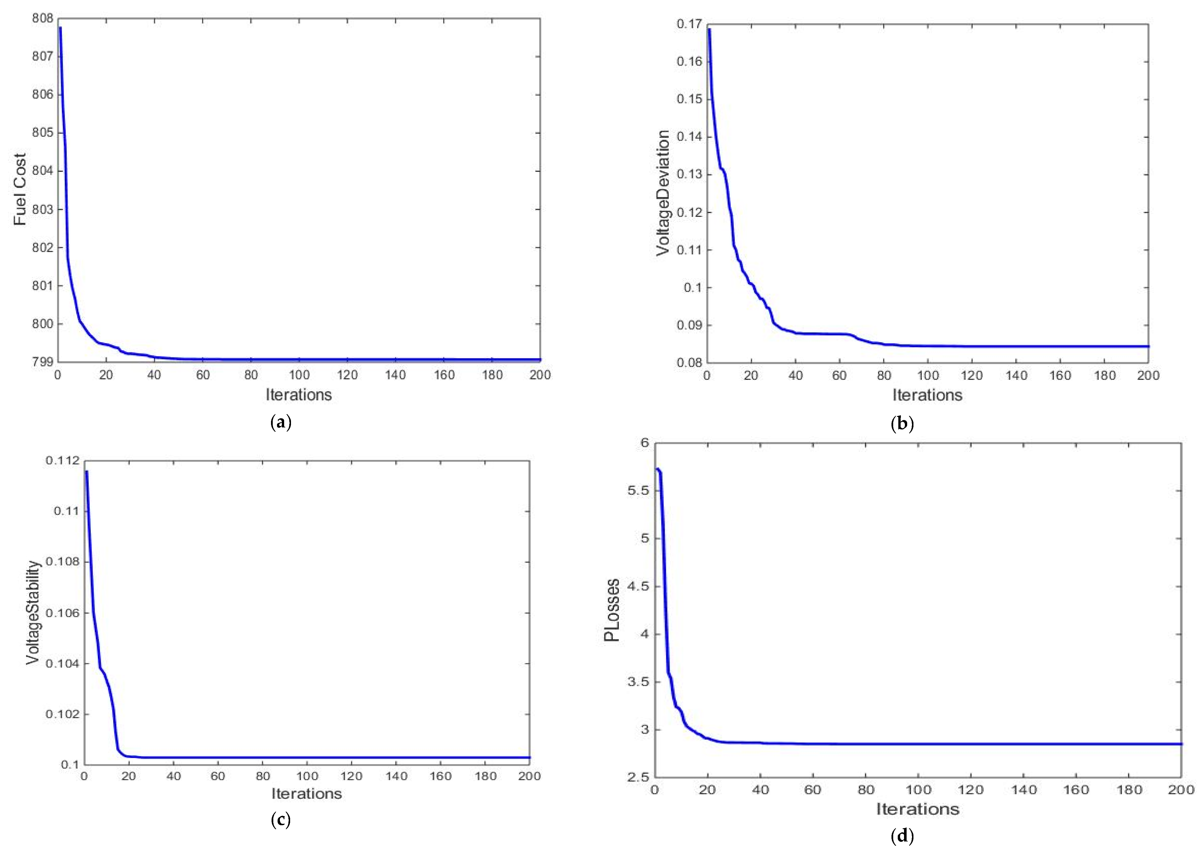
QC29 (Mvar)	0	5	2.77	2.91	5.00	2.53	2.62

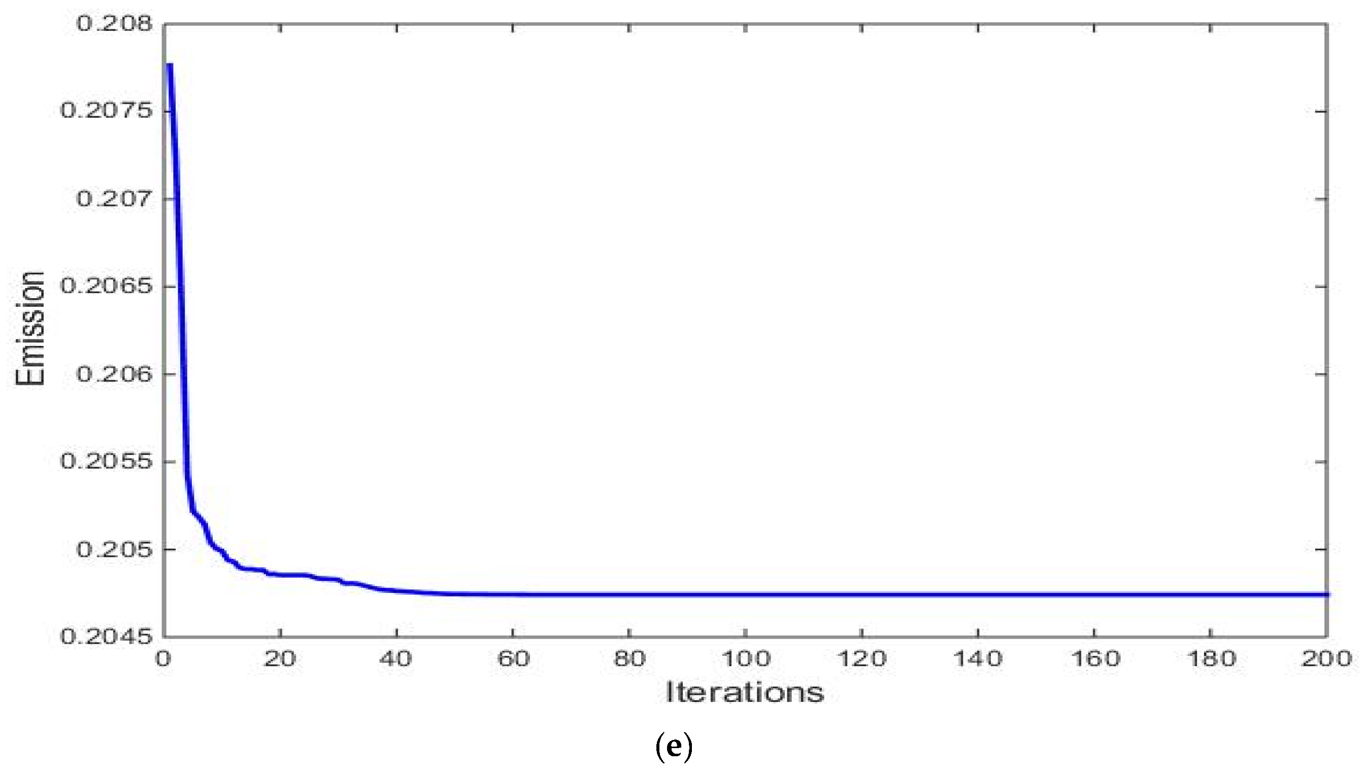
for the complete control variables for Cases 1–5. In Case 1, the objective function aims to minimize the fuel cost. The reported fuel cost equals 799.071 $/h. In Case 2, the main objective is minimizing the voltage deviation at all load buss. The VD equals 0.084 p.u using the TFWO algorithm. In Case 3, the reported voltage stability index is 0.1 p.u. The minimum power losses obtained in Case 4 is 2.851 MW. The lowest emission rate is obtained in Case 5 (0.205 ton/kg).

Table 3. TFWO versus recent optimization algorithms for single objective functions for the IEEE 30-bus test system.

Case #	PSO-SSO [29]	SSO [29]	PSO [29]	DA-PSO [45]	DA-APSO [46]	ECHT [57]	MVO [60]	WOA-PS [49]	TFWO
1	798.98	799.41	801.23	802.12	802.63	800.41	799.24	799.56	799.071
2	1.25	1.54	1.61	-	-	-	-	-	0.084
3	0.124	0.125	0.125	-	-	0.136	0.115	-	0.100
4	2.858	2.902	3.278	3.189	3.003	3.084	2.881	2.967	2.851
5	0.205	0.205	0.205	0.205	-	0.205	-	0.206	0.205

shows a comparison between the TFWO and some recent optimization algorithms from the literature for Cases 1–5. It is clear that the proposed TFWO leads to the most competitive solutions for different objectives.

The lowest value of voltage deviation (0.084 p.u) for Case 2 is via the proposed TFWO. In addition, the best voltage stability index, the lower value of power losses, and a notable improvement in emission level are noticed using TFWO compared to the literature works. Figure 1 shows good convergence rates using the proposed TFWO for all studied cases in finding the optimal solution of single objective functions, Cases 1–5. The convergence curves show that the TFWO reaches the optimal solution fast and stay stable, and we noted that reaching the optimal solution occurred within 10–20% of the total number of iterations.

-

Results of bi-objective cases

Table 4. Optimal power flow solution for IEEE-30 bus system using the TFWO algorithm for Cases 6–14.

VARs	Case #6	Case #7	Case #8	Case #9	Case #10	Case #11	Case #12	Case #13	Case #14
Fuel cost ($/h)	835.074	840.918	799.072	803.416	862.639	864.151	804.318	826.779	826.566
VD (p.u.)	2.024	2.033	1.911	0.101	0.323	2.039	0.143	0.459	0.444
VS	0.115	0.115	0.115	0.137	0.136	0.115	0.137	0.134	0.134
PL (MW)	5.034	4.711	8.626	9.795	4.515	4.100	8.419	5.459	5.520
Emission (ton/h)	0.242	0.240	0.366	0.365	0.227	0.224	0.325	0.255	0.254

shows the simulation results of bi-, tri-, and quad-objective functions for Cases 6–14, while

Table A2. Control variables of IEEE-30 bus system using TFWO algorithm for Cases 6–14.

VARs	Case #6	Case # 7	Case # 8	Case # 9	Case # 10	Case #11	Case # 12	Case # 13	Case # 14
PG1 (MW)	112.93	112.80	177.05	176.64	100.79	96.82	160.92	123.17	121.86
PG2 (MW)	58.97	53.35	48.70	48.86	56.18	58.25	51.56	53.64	55.95
PG5 (MW)	27.62	33.67	21.30	21.62	38.93	37.50	22.58	30.03	28.38
PG8 (MW)	35.00	35.00	21.09	21.90	35.00	35.00	27.90	35.00	35.00
PG11 (MW)	27.27	30.00	11.88	12.18	30.00	30.00	14.91	25.86	25.33
PG13 (MW)	26.64	23.30	12.00	12.00	27.02	29.93	13.95	21.16	22.41
V1 (p.u.)	1.10	1.10	1.10	1.05	1.07	1.10	1.06	1.10	1.10
V2 (p.u.)	1.09	1.09	1.09	1.03	1.06	1.09	1.04	1.09	1.09
V5 (p.u.)	1.07	1.07	1.06	1.01	1.04	1.07	1.00	1.06	1.06
V8 (p.u.)	1.08	1.08	1.07	1.00	1.05	1.08	1.01	1.07	1.07
V11 (p.u.)	1.10	1.10	1.10	1.02	1.03	1.10	1.05	1.01	1.01
V13 (p.u.)	1.10	1.10	1.10	0.99	1.02	1.10	1.02	1.03	1.03
T6-9	1.04	1.04	1.04	1.04	1.10	1.04	1.07	1.10	1.10
T6-10	0.90	0.90	0.90	0.90	0.94	0.90	0.90	0.99	0.98
T4-12	0.98	0.98	0.98	0.95	1.04	0.98	1.00	1.07	1.07
T28-27	0.97	0.97	0.96	0.97	1.01	0.97	0.97	1.04	1.03
QC10 (Mvar)	5.00	5.00	5.00	4.99	0.02	5.00	1.69	5.00	4.99
QC12 (Mvar)	5.00	5.00	5.00	5.00	0.00	5.00	0.00	0.00	0.00
QC15 (Mvar)	5.00	5.00	5.00	5.00	5.00	4.94	4.69	4.05	3.85
QC17 (Mvar)	5.00	5.00	5.00	0.00	4.32	5.00	1.00	5.00	4.86
QC20 (Mvar)	5.00	5.00	5.00	5.00	5.00	5.00	5.00	5.00	5.00
QC21 (Mvar)	5.00	5.00	5.00	5.00	5.00	5.00	5.00	5.00	5.00
QC23 (Mvar)	3.91	3.83	4.76	5.00	3.63	3.53	4.80	4.07	4.41
QC24 (Mvar)	5.00	5.00	5.00	5.00	5.00	5.00	5.00	5.00	5.00
QC29 (Mvar)	2.66	2.66	2.94	2.57	2.51	2.61	1.91	2.59	2.32

shows the settings of various control variables for the tested cases. The Cases 6–9 represent the bi-objective cases. The fuel costs and emissions level are optimized simultaneously in Case 6. Case 7 optimizes the fuel costs and power losses. The fuel costs and the voltage stability index are considered in Case 8, while Case 9 optimizes the fuel costs and the voltage deviation as the primary bi- objectives. The simulation results using the proposed TFWO algorithm are compared to other related works in the literature [46,53,58,61,62,64].

Table 5. TFWO versus recent optimization algorithms from the literature for multi-objective functions for (Cases 6–9).

Case #	Objective	MSA [61]	PSO [29]	EMSA [61]	MODA [58]	DA-APSO [46]	MOFA-CPA [62]	PSO-SSO [29]	ECHIT [57]	TFWO
6	Fuel Cost	834.1532	834.95	8.33.977	8.38.604	-	852.02	834.80	-	835.074
	Emission	0.3286	0.243	0.3293	0.254	-	0.279	0.243	-	0.242
7	Fuel Cost	856.2673	-	859.9514	-	-	-	-	-	840.918
	Power Loss	9.9012	-	4.9012	-	-	-	-	-	4.711
8	Fuel cost	800.0275	834.4	799.3582	-	-	-	830.35	-	799.072
	Voltage Stability	0.1209	0.128	0.1209	-	-	-	0.125	-	0.115
9	Fuel cost	803.8740	804.48	803.4286	807.2807	802.63	-	803.99	803.72	803.416
	Voltage Deviation	0.1180	0.126	803.8740	0.023	0.116	-	0.094	0.095	0.101

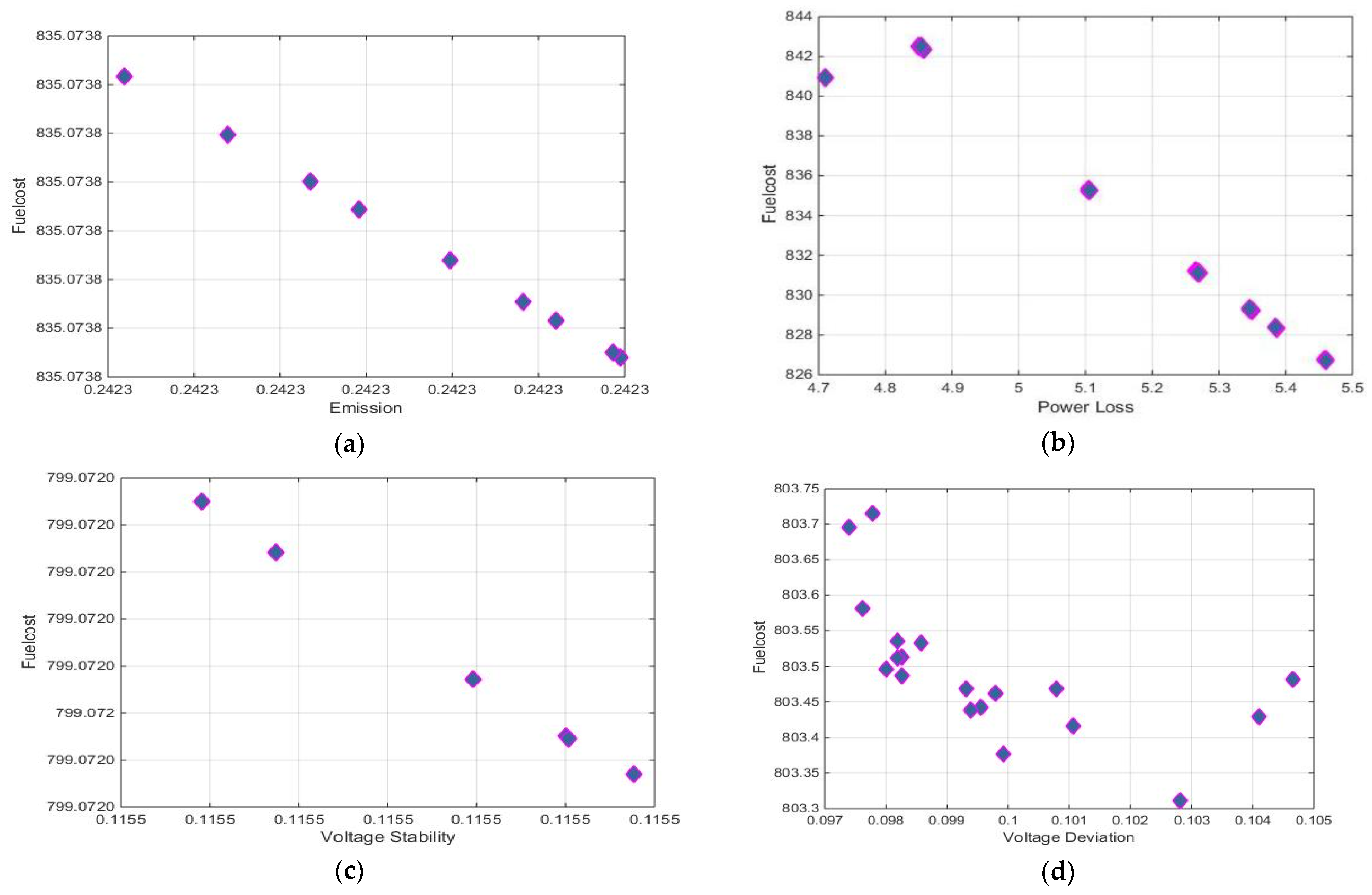
shows that the proposed TFWO leads to the most efficient solutions for Cases 6–9. Figure 2 shows Pareto sets for Cases 6–9.

-

Results of the triple-objective cases

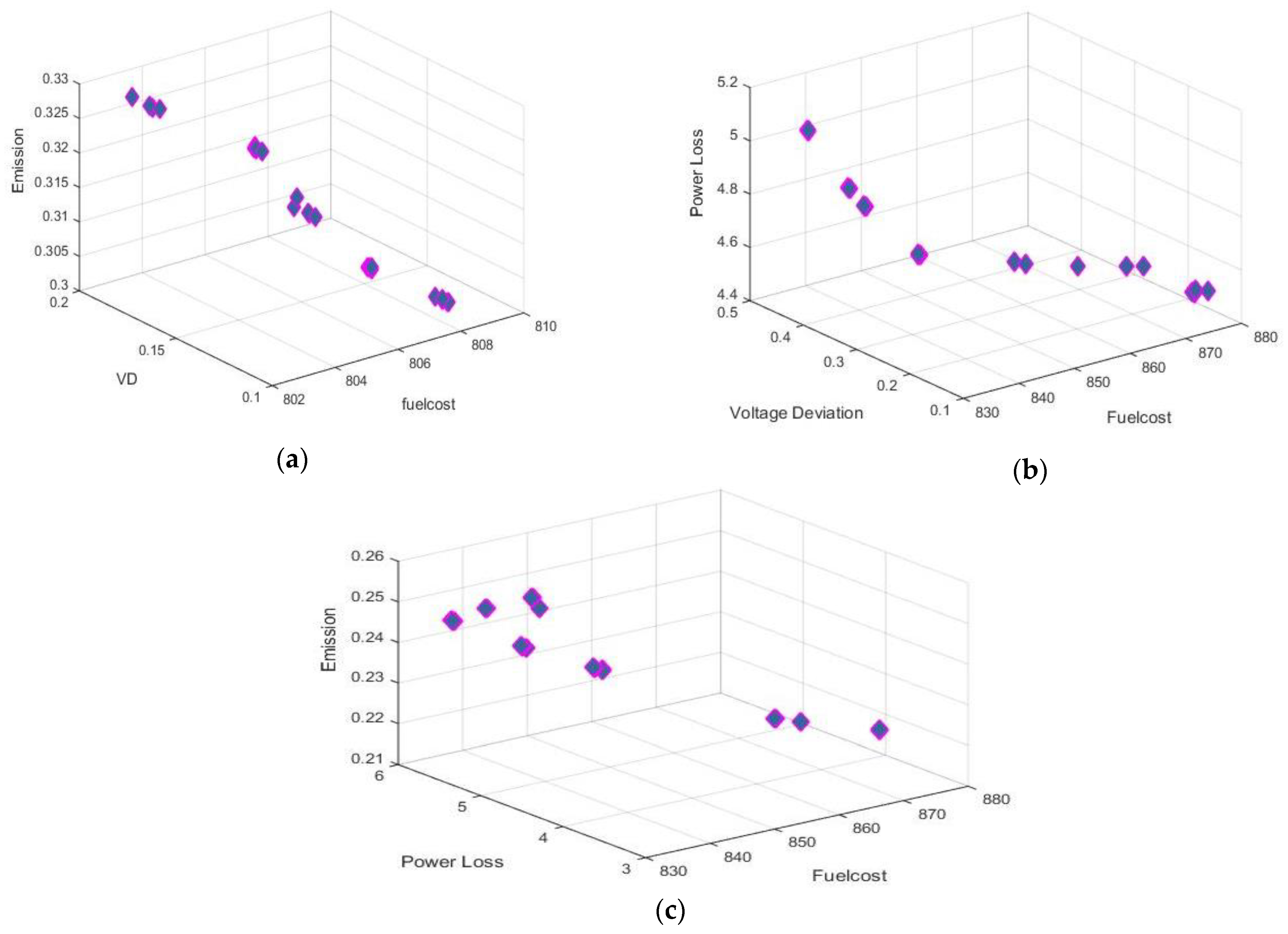
The triple-objective cases are considered in Cases 10–12. Table 4 shows the simulation results reported for these cases using the proposed TFWO algorithm. In Case 10, three objectives, fuel costs, voltage deviation, and power losses are optimized simultaneously. In Case 11, the triple function aims at minimizing the fuel costs, the power losses and the emission level, while Case 12 optimizes the fuel costs, the voltage deviation, and the emission level simultaneously.

The efficiency of the proposed TFWO algorithm is confirmed by comparing the simulated results obtained with other studies in literature [53,58,59,62,64]. It is clear from

Table 6. TFWO versus recent optimization algorithms for tri-objective functions (IEEE-30 bus test system) Cases (10–12).

Case #	Objectives	PSO [29]	MODA [58]	SSO [29]	Jaya [59]	MOFA-CPA [62]	PSO-SSO [29]	TFWO
10	Fuel Cost	889.58	-	858.88	826.44	-	864.27	862.639
	Voltage Deviation	0.353	-	0.353	0.2662	-	0.316	0.323
	Power Loss	4.712	-	4.712	6.611	-	4.545	4.515
11	Fuel Cost	864.584	867.907	867.034	858.9	878.13	865.18	864.151
	Power Loss	4.197	4.5342	4.148	4.622	3.9232	4.093	4.100
	Emission	0.225	0.2640	0.223	0.233	0.2165	0.224	0.224
12	Fuel cost	814.833	-	807.94	834.06	-	804.332	804.318
	Voltage Deviation	0.156	-	0.166	0.1989	-	0.164	0.143
	Emission	0.343	-	0.313	0.2511	-	0.346	0.325

that the proposed TFWO leads to enhanced fuel costs and power losses, while an increase in voltage deviation is reported compared to PSO-SSO [53] for Case 10. In addition, the economic/technical and environmental benefits are enhanced in Cases 11–12 compared to PSO, SSO, PSO-SSO [53], and MOAD [58]. Pareto solutions of Cases 10–12 are shown in Figure 3.

-

Results of the multi-objectives cases

Table 7. TFWO versus recent optimization algorithms for Cases 13 and 14 (IEEE-30 bus test system).

Case #	Objectives	PSO [29]	MODA [58]	ECHIT [57]	I-NSGA-III [63]	SSO [29]	Jaya [59]	PSO-SSO [29]	TFWO
13	Fuel Cost	828.29	828.49	803.21	881.9395	829.978	-	826.94	826.779
	Voltage Deviation	0.55	0.585	0.296	0.1754	0.516	-	0.466	0.459
	Power Loss	5.644	5.912	5.586	4.7449	5.426	-	5.515	5.459
	Emission	0.261	0.265	0.253	0.2209	0.25	-	0.258	0.255
14	Fuel Cost	828.29	-	-	843.8571	827.78	812.18	826.8	826.566
	Voltage Deviation	0.55	-	-	0.2388	0.55	0.1905	0.463	0.444
	Voltage Stability	0.25	-	-	0.1253	0.145	0.1343	0.145	0.134
	Power Loss	5.644	-	-	5.7405	5.644	9.003	5.464	5.520
	Emission	0.261	-	-	0.1485	0.261	0.3162	0.256	0.254

shows a comparison between simulation results using TFWO and others. Case 13 optimizes the fuel costs, voltage deviation, power losses, and emission level simultaneously. The five objective functions are considered in Case 14. Acceptable economic, technical and environmental benefits are obtained compared to the competitive PSO-SSO and MODA in Cases 13 and 14. The effectiveness and ability of the proposed TFWO are confirmed through these comparison studies with well-known competitive algorithms.

5.2. Simulation Results of IEEE 57-Bus System

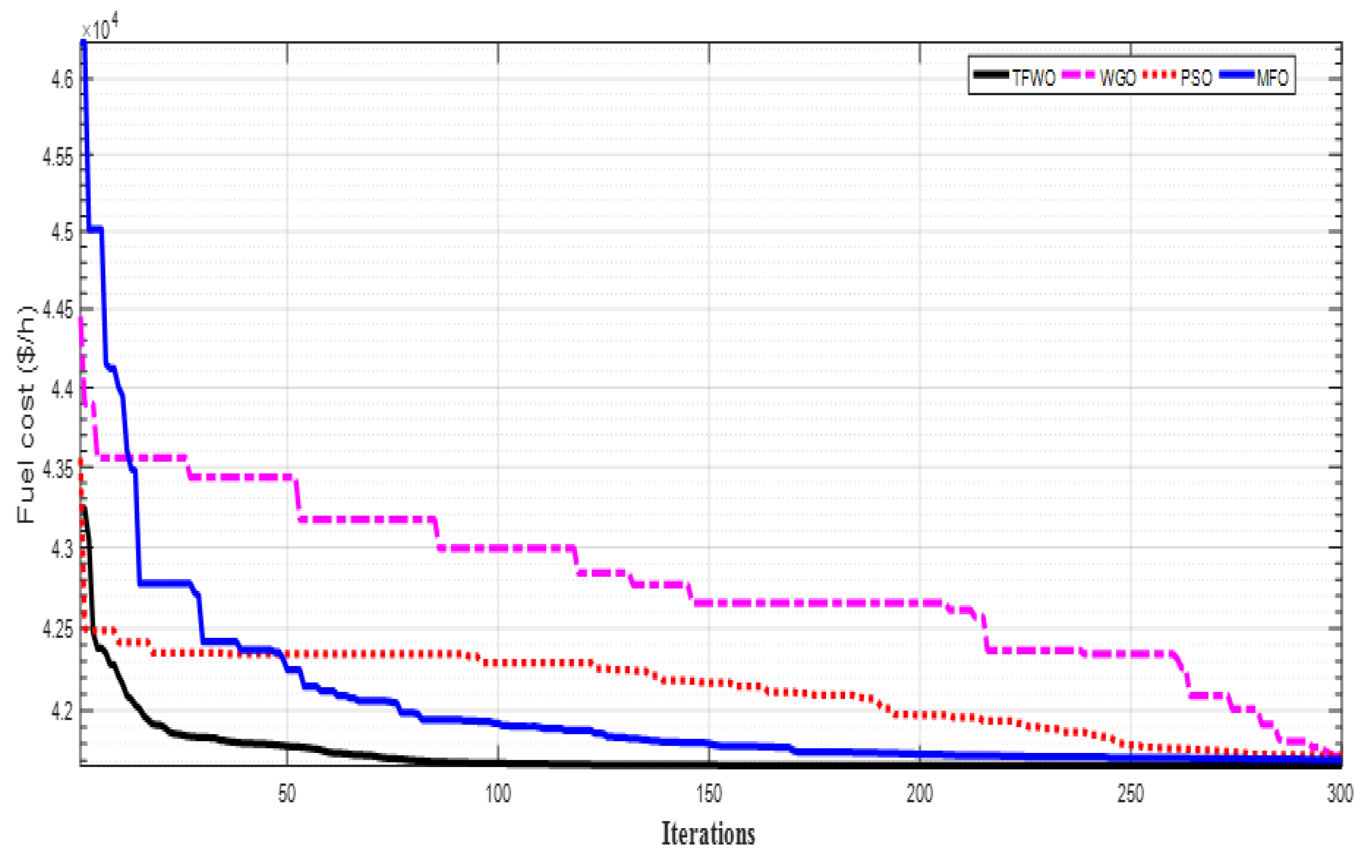
The IEEE 57-bus system consists of 7-generation buses, 80 branches. It has 17 tap changers (at branches 19, 20, 31, 35, 36, 37, 41, 46, 54, 58, 59, 65, 66, 71, 73, 76, and 80) with upper and lower bounds at 1.1–0.9 p.u. There are three shunt reactive sources located at buses 18, 25, and 53 with bounds of 0.2–0.0 in p.u. The boundaries for voltages of all generator buses are considered as 1.05–0.95 p.u. The scalability of the TFWO algorithm was tested on IEEE 57-bus system to investigate the ability to solve single and multi-objectives in large system. The population is 100, and the maximum number of iterations is 300. The OPF problem was solved for three cases: two single objective and a multi-objective. A single objective function is considered in Cases 15 and 16 for minimizing the fuel costs and power losses, respectively. In Case 17, bi-objectives were considered to optimize fuel costs and power losses simultaneously.

Cases 15–17 were optimized using three competitive algorithms GWO, PSO, and MFO in addition to the proposed TFWO. The simulation results of the proposed TFWO algorithm were compared to the competitive algorithms to prove the ability, efficiency and the effectiveness of the proposed method.

Table 8. TFWO versus recent optimization algorithms (IEEE-57 bus test system) for Cases 15–17.

Case	Case 15 (Minimum Fuel Cost)				Case 16 (Minimum Power Loss)				Case 17 (Min. Fuel Cost& Power Loss)
Algorithm	TFWO	GWO	PSO	MFO	TFWO	GWO	PSO	MFO	TFWO	GWO	PSO	MFO
Fuel cost ($/h)	41,667.07	41,726.48	41,727.01	41,695.265	49,532.74	47,225.36	48,126.98	49,360.1	41,702.0	41,965.6	41,905.8	41,792.5
Emission (ton/h)	1.3492	1.403	1.39046	1.364	0.94773	0.9494	0.94937	0.94795	1.32	1.4266	1.3489	1.304
$p_{loss}(\mathrm{MW})$	14.847	15.83	16.159	15.266	11.18	11.994	11.997	11.295	13.89	13.793	13.715	13.914

shows the OPF simulation results obtained for Cases 15–17 using the proposed TFWO algorithm and the other three competitive algorithms. In Case 15, the minimum fuel costs were 41,667.07 $/h with TFWO and 41,804.91, 41,727.01, and 41,708.38 $/h with GOW, PSO, and MFO, respectively. It is clear that the minimum fuel costs obtained is via TFWO. The active power loss in Case 16 was reported as 11.18 MW using the proposed TFWO. In Case 17, the best results obtained using TFWO (41,702.0 $/h and 13.89 MW).

Table 9. TFWO versus recent optimization algorithms for IEEE-57 bus test system: Cases 15–17.

Case #	OF	GWO	PSO	MFO	SFLA [65]	GSA [16]	ABC [66]	DA_PSO [46]	MSA [61]	EMSA [61]	TFWO
15	FC	41,726.48	41,727.01	41,695.26	41,872.9	41,695	41,781	41,674.6	41,673.59	41,666.2	41,667.07
16	PL	11.994	11.997	11.295	-	-	12.626	10.1212	-	-	11.18
17	FC	41965.6	41905.8	41792.5	-	-	-	-	-	-	41702.0
	PL	13.793	13.89	13.914	-	-	-	-	-	-	13.89

presents a comparison of TFWO to recent well-known algorithms in literature. Moreover, the convergence rate of TFWO compared to the three competitive algorithms are shown in Figure 4. It is clear from the convergence curves that TFWO has the faster convergence rate compared with the others. Statistical indices applied on Case 15 for 50 runs of each algorithm are extracted in

Table 10. Statistical performance evaluation of TFWO for Case 15 compared with three optimizers.

Methods	Minimum FC ($/h)—50 Trials
	Min.	Max.	Mean	Variance	Median	STD
GWO	41,726.484	42,359.511	41,923.641	17,137.912	41,903.810	130.912
PSO	41,727.013	42,396.201	42,014.195	32,359.361	42,018.992	179.887
MFO	41,695.265	42,102.002	41,811.571	8543.453	41,795.430	92.431
TFWO	41,667.076	41,699.594	41,678.955	98.648	41,675.142	9.932

. It is noticed again that TFWO has the best fuel costs, the lower variance and standard deviation (STD) considered as a good indicator for the efficiency and effectiveness of the proposed TFWO algorithm.

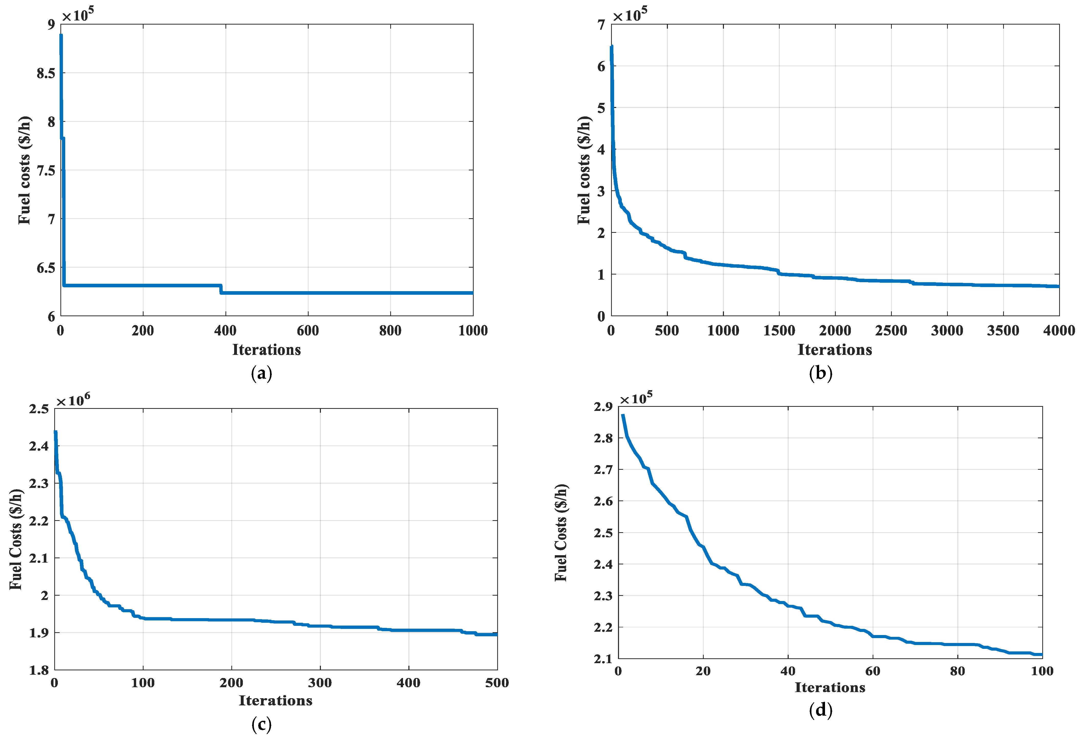
5.3. Simulation Results for Large Scale Test Systems

Four additional large scale test systems are employed to validate the proposed TFWO (Cases 18–21). These systems have varied number of buses power systems. The main data for each tested system is customized from the MATPOWER 6.2 package [67].

The first large scale system is called the IEEE 300-bus test system. The IEEE 300-bus system consists of 69-generating units and 411 branches. The system supplies a demand apparent power of (23,525.85 + j 7780) MVA. This test system consists of 259 control variables. These variables are 69 active powers of generating units, 69 voltage magnitudes of generating buses, 107 tap changers, and 14 shunt reactive sources for reactive power compensation. The upper and lower bounds of voltage magnitudes are at 1.1–0.95 p.u. The tap changers of transformers are regulated with the limits of [1.1–0.9].

The second large power system network is called 1354pegase test case. This system consists of 1354 buses, 260 generators, and 1991 branches. The system supplies a demand apparent power of (73,059.7 + j 13,401.4) MVA. This test system consists of 1836 control variables. These variables are 260 active power of generating units, 260 voltage magnitudes of generating buses, 234 tap changers, and 1082 shunt reactive sources for reactive power compensation. The upper and lower bounds of voltage magnitudes are at 1.1–0.9 p.u. The tap changers of transformers are regulated with the limits of [1.1–0.9].

The third large scale test system is called IEEE 3012 bus test system. This system consists of 3012 buses, 502 generators, and 3572 branches. The system supplies a demand apparent power of (27,169.7 + j 10,200.6) MVA. This test system consists of 1214 control variables. These variables are 502 active powers of generating units, 502 voltage magnitudes of generating buses, 201 tap changers, and nine shunt reactive sources for reactive power compensation. The upper and lower bounds of voltage magnitudes are at 1.1–0.95 p.u. The tap changers of transformers are regulated with the limits of [1.1–0.9]. The fourth large scale test system is called IEEE 9241pegase test system.

This system consists of 9241 buses, 1445 generator, 16,049 branches. The system supplies a demand apparent power of (312,354.1 + j 73,581.6) MVA. This test system consists of 11,536 control variables. These variables are 1445 active power of generating units, 1445 voltage magnitudes of generating buses, 1319 tap changers, and 7327 shunt reactive sources for reactive power compensation. The upper and lower bounds of voltage magnitudes are at 1.1–0.90 p.u. The tap changers of transformers are regulated with the limits of [1.1–0.9]. The data of these systems are customized from Matpower6.0b2 software [67]. The four large scale systems are optimized to minimize the fuel costs of generating units for Cases 18–21 as reported in Table 1.

Table 11. TFWO versus recent optimization algorithms for the IEEE large scale test system: Cases 18–21.

Case #	Objectives	System	MATPOWER [67]	TFWO	Reduction%
18	Fuel Cost	IEEE 300-bus	719,692.27 $/h	623,581.39 $/h	13.4%
19		IEEE 1354-bus	74,069.35 $/h	70,810.49 $/h	4.4%
20		IEEE 3012-bus	2,591,706.57	1,894,369.136	27%
21		IEEE 9241pegase	315,912.43 $/h	211,308.43$/h	33.12%

shows the simulation results of the proposed TFWO compared to the results of the Matpower6.0b2 simulator for the four large scale test systems to validate the scalability and efficiency of the TFWO algorithm. For the IEEE 300-bus test system, the fuel costs obtained using the TFWO (623,581.39 $/h) are compared with those obtained by the MATPOWER (719,692.27 $/h).

A reduction of 13.4% is achieved by the proposed TFWO. For the IEEE 1354-bus test system, the objective function of fuel costs obtained using the proposed TFWO is 70,810.49 $/h compared to 74,069.35 $/h using the Matpower6.0b2 simulator. A reduction of 4.6% is achieved by the proposed TFWO. For the third large scale system, the fuel costs obtained using the proposed TFWO is 1894369.136 $/h compared to 2,591,706.57 $/h $/h using the Matpower6.0b2 simulator with a reduction of 27%. For the fourth large scale test system, the fuel costs using the proposed TFWO equals 211,308.43 $/h compared to 315,912.43 $/h $/h using the Matpower6.0b2.

A reduction of 33.12% is achieved by the proposed TFWO. Figure 5 shows the convergence rates for the tested large-scale systems. From the previous simulation results, the proposed TFWO is validated on small- and large-scale test systems. All results obtained emphasize that the TFWO algorithm outperforms the others and has a fast, smooth and stable convergence rate with the increased variables number. These are acceptable techno-economic benefits compared with previous methods as the economical reduction lies in the range of 4.6–33.12%.

6. Conclusions

In this paper, a novel meta-heuristic intelligent algorithm called TFWO algorithm has been implemented to solve OPF problem for small and large systems. Single and multi-objective functions were employed to minimize the cost of fuel, emission level, power losses, enhance voltage deviation and voltage stability index. The proposed algorithm was tested and investigated on the IEEE 30-bus and 57-bus systems and seventeen different cases.

Evaluation of the effectiveness and robustness of the proposed TFWO algorithm was conducted through a comparison of the simulation results, convergence rate, and statistical indices to other well-known recent algorithms in the literature. Statistical indices showed that TFWO had the best fuel costs, the lower average, variance, and standard deviation that also considered indicators for the effectiveness and accuracy of the proposed algorithm. The scalability of the proposed algorithm was validated through optimizing the IEEE 300-bus, IEEE 1354-bus, IEEE 3012-bus, and IEEE 9241pegase test systems.

A reduction in the fuel costs reached 4.6% in the IEEE 1354-bus, and its level increased for the IEEE-bus 300-bus and for IEEE 9241pegase test system to 13.4% and 33.12%, respectively. The simulation results at the small, medium, and large test system emphasize that TFWO algorithm is efficient, effective, robust and superior in solving OPF optimization problems. It had a better convergence rate than other well-known algorithms that make it an outperforming algorithm in complex engineering problems.

The main weakness is the solution concentration particularly with the increase of the system size. The problem was solved under normal operation only. In this direction, two future trends can be considered to extend this study. The first one aims at solving the OPF in the emergency events such as the outage of one or more generation units and the outage of transmission networks. The second trend is the development of recent optimization algorithms to solve the target problem.

References

1. Rizk-Allah, R.M.; El-Sehiemy, R.A. A novel sine cosine approach for single and multiobjective emission/economic load dispatch problem. In Proceedings of the International Conference on Innovative Trends in Computer Engineering (ITCE 2018), Aswan, Egypt, 15 June 2017; pp. 271–277. [Google Scholar]
2. Shaheen, A.M.; Farrag, S.M.; El-Sehiemy, R.A. MOPF solution methodology. IET Gener. Transm. Distrib. 2017, 11, 570–581. [Google Scholar] [CrossRef]
3. Buch, H.; Trivedi, I.N.; Jangir, P. Moth flame optimization to solve optimal power flow with non-parametric statistical evaluation validation. Cogent Eng. 2017, 4, 1286731. [Google Scholar] [CrossRef]
4. Mohammadi, A.; Kargarian, A. Accelerated and Robust Analytical Target Cascading for Distributed Optimal Power Flow. IEEE Trans. Ind. Inform. 2020, 16, 7521–7531. [Google Scholar] [CrossRef]
5. You, L.; Ma, H.; Saha, T.; Liu, G. Risk-based Contingency-constrained Optimal Power Flow with Adjustable Uncertainty Set of Wind Power. IEEE Trans. Ind. Inform. 2021, 18, 996–1008. [Google Scholar] [CrossRef]
6. Nguyen, T.T.; Vo, D.N.; Van Tran, H.; Van Dai, L. Optimal dispatch of reactive power using modified stochastic fractal search algorithm. Complexity 2019, 2019, 4670820. [Google Scholar] [CrossRef]
7. Biswas, P.P.; Suganthan, P.N.; Mallipeddi, R.; Amaratunga, G.A.J. Optimal reactive power dispatch with uncertainties in load demand and renewable energy sources adopting scenario-based approach. Appl. Soft Comput. 2019, 75, 616–632. [Google Scholar] [CrossRef]
8. Shafik, M.B.; Rashed, G.I.; El-Sehiemy, R.A.; Chen, H. Optimal Sizing and Sitting of TCSC Devices for Multi-Objective Operation of Power Systems Using Adaptive Seeker Optimization Algorithm. In Proceedings of the Region 10 Symposium, Tensymp 2018, Sydney, Australia, 4–6 July 2018; pp. 231–236. [Google Scholar]
9. Saddique, M.S.; Bhatti, A.R.; Haroon, S.S.; Sattar, M.K.; Amin, S.; Sajjad, I.A.; ul Haq, S.S.; Awan, A.B.; Rasheed, N. Solution to optimal reactive power dispatch in transmission system using meta-heuristic techniques―Status and technological review. Electr. Power Syst. Res. 2020, 178, 106031. [Google Scholar] [CrossRef]
10. Suresh, V.; Kumar, S.S. Optimal reactive power dispatch for minimization of real power loss using SBDE and DE-strategy algorithm. J. Ambient Intell. Humaniz. Comput. 2020, 1–15. [Google Scholar] [CrossRef]
11. Chaib, A.E.; Bouchekara, H.R.E.H.; Mehasni, R.; Abido, M.A. Optimal power flow with emission and non-smooth cost functions using backtracking search optimization algorithm. Int. J. Electr. Power Energy Syst. 2016, 81, 64–77. [Google Scholar] [CrossRef]
12. Shaukat, N.; Ahmad, A.; Mohsin, B.; Khan, R.; Khan, S.U.-D.; Khan, S.U.-D. Multiobjective Core Reloading Pattern Optimization of PARR-1 Using Modified Genetic Algorithm Coupled with Monte Carlo Methods. Sci. Technol. Nucl. Install. 2021, 2021, 1802492. [Google Scholar] [CrossRef]
13. Cao, Y.; Zhang, H.; Li, W.; Zhou, M.; Zhang, Y.; Chaovalitwongse, W.A. Comprehensive learning particle swarm optimization algorithm with local search for multimodal functions. IEEE Trans. Evol. Comput. 2018, 23, 718–731. [Google Scholar] [CrossRef]
14. Zhao, B.; Guo, C.X.; Cao, Y.J. A multiagent-based particle swarm optimization approach for optimal reactive power dispatch. IEEE Trans. Power Syst. 2005, 20, 1070–1078. [Google Scholar] [CrossRef]
15. Naderi, E.; Narimani, H.; Fathi, M.; Narimani, M.R. A novel fuzzy adaptive configuration of particle swarm optimization to solve large-scale optimal reactive power dispatch. Appl. Soft Comput. 2017, 53, 441–456. [Google Scholar] [CrossRef]
16. Duman, S.; Sönmez, Y.; Güvenç, U.; Yörükeren, N. Optimal reactive power dispatch using a gravitational search algorithm. IET Gener. Transm. Distrib. 2012, 6, 563–576. [Google Scholar] [CrossRef]
17. Ayan, K.; Kılıç, U. Artificial bee colony algorithm solution for optimal reactive power flow. Appl. Soft Comput. 2012, 12, 1477–1482. [Google Scholar] [CrossRef]
18. Ettappan, M.; Vimala, V.; Ramesh, S.; Kesavan, V.T. Optimal reactive power dispatch for real power loss minimization and voltage stability enhancement using Artificial Bee Colony Algorithm. Microprocess. Microsyst. 2020, 76, 103085. [Google Scholar] [CrossRef]
19. Sulaiman, M.H.; Mustaffa, Z.; Mohamed, M.R.; Aliman, O. Using the gray wolf optimizer for solving optimal reactive power dispatch problem. Appl. Soft Comput. J. 2015, 32, 286–292. [Google Scholar] [CrossRef] [Green Version]
20. Jamal, R.; Men, B.; Khan, N.H. A novel nature inspired meta-heuristic optimization approach of GWO optimizer for optimal reactive power dispatch problems. IEEE Access 2020, 8, 202596–202610. [Google Scholar] [CrossRef]
21. Mei, R.N.S.; Sulaiman, M.H.; Mustaffa, Z.; Daniyal, H. Optimal reactive power dispatch solution by loss minimization using moth-flame optimization technique. Appl. Soft Comput. 2017, 59, 210–222. [Google Scholar]
22. Mouassa, S.; Bouktir, T.; Salhi, A. Ant lion optimizer for solving optimal reactive power dispatch problem in power systems. Eng. Sci. Technol. Int. J. 2017, 20, 885–895. [Google Scholar] [CrossRef]
23. Barakat, A.F.; El-Sehiemy, R.A.; Elsaid, M.; Osman, E. Solving Reactive Power Dispatch Problem by Using JAYA Optimization Algorithm. Int. J. Eng. Res. Afr. 2018, 36, 12–24. [Google Scholar] [CrossRef]
24. Ebeed, M.; Alhejji, A.; Kamel, S.; Jurado, F. Solving the Optimal Reactive Power Dispatch Using Marine Predators Algorithm Considering the Uncertainties in Load and Wind-Solar Generation Systems. Energies 2020, 13, 4316. [Google Scholar] [CrossRef]
25. Khelifi, A.; Bentouati, B.; Chettih, S.; Sehiemy, R.A.E. Application of Hybrid Salp Swarm optimization Method for Solving OPF Problem. In Proceedings of the International Conference on Advanced Electrical Engineering 2019 (ICAEE 2019), Algiers, Algeria, 19–21 November 2019. [Google Scholar]
26. Shafik, M.B.; Chen, H.; Rashed, G.I.; El-Sehiemy, R.A.; Elkadeem, M.R.; Wang, S. Adequate topology for efficient energy resources utilization of active distribution networks equipped with soft open points. IEEE Access 2019, 7, 99003–99016. [Google Scholar] [CrossRef]
27. Ela, A.A.A.E.; El-Sehiemy, R.A.; Shaheen, A.M.; Shalaby, A.S. Application of the crow search algorithm for economic environmental dispatch. In Proceedings of the 19th International Middle-East Power Systems Conference (MEPCON 2017), Cairo, Egypt, 19–21 December 2017; pp. 78–83. [Google Scholar]
28. Rizk-Allah, R.M.; Mageed, H.M.A.; El-Sehiemy, R.A.; Aleem, S.H.E.A.; El Shahat, A. A new sine cosine optimization algorithm for solving combined non-convex economic and emission power dispatch problems. Int. J. Energy Convers. 2017, 5, 180–192. [Google Scholar] [CrossRef]
29. El Sehiemy, R.A.; Selim, F.; Bentouati, B.; Abido, M.A. A novel multi-objective hybrid particle swarm and salp optimization algorithm for technical-economical-environmental operation in power systems. Energy 2020, 193, 116817. [Google Scholar] [CrossRef]
30. Abdul-Hamied, D.T.; Shaheen, A.M.; Salem, W.A.; Gabr, W.I.; El-Sehiemy, R.A. Equilibrium optimizer based multi dimensions operation of hybrid AC/DC grids. Alex. Eng. J. 2020, 59, 4787–4803. [Google Scholar] [CrossRef]
31. Mugemanyi, S.; Qu, Z.; Rugema, F.X.; Dong, Y.; Bananeza, C.; Wang, L. Optimal reactive power dispatch using chaotic bat algorithm. IEEE Access 2020, 8, 65830–65867. [Google Scholar] [CrossRef]
32. Subbaraj, P.; Rajnarayanan, P.N. Optimal reactive power dispatch using self-adaptive real coded genetic algorithm. Electr. Power Syst. Res. 2009, 79, 374–381. [Google Scholar] [CrossRef]
33. Dai, C.; Chen, W.; Zhu, Y.; Zhang, X. Seeker optimization algorithm for optimal reactive power dispatch. IEEE Trans. Power Syst. 2009, 24, 1218–1231. [Google Scholar] [CrossRef]
34. Bai, W.; Eke, I.; Lee, K.Y. An improved artificial bee colony optimization algorithm based on orthogonal learning for optimal power flow problem. Control Eng. Pract. 2017, 61, 163–172. [Google Scholar] [CrossRef]
35. El-Fergany, A.A.; Hasanien, H.M. Single and Multi-objective Optimal Power Flow Using Grey Wolf Optimizer and Differential Evolution Algorithms. Electr. Power Compon. Syst. 2015, 43, 1548–1559. [Google Scholar] [CrossRef]
36. Abdo, M.; Kamel, S.; Ebeed, M.; Yu, J.; Jurado, F. Solving non-smooth optimal power flow problems using a developed grey wolf optimizer. Energies 2018, 11, 1692. [Google Scholar] [CrossRef] [Green Version]
37. Taher, M.A.; Kamel, S.; Jurado, F.; Ebeed, M. An improved moth-flame optimization algorithm for solving optimal power flow problem. Int. Trans. Electr. Energy Syst. 2019, 29, e2743. [Google Scholar] [CrossRef]
38. Islam, M.Z.; Wahab, N.I.A.; Veerasamy, V.; Hizam, H.; Mailah, N.F.; Khan, A.; Sabo, A. Optimal Power Flow using a Novel Harris Hawk Optimization Algorithm to Minimize Fuel Cost and Power loss. In Proceedings of the 2019 IEEE Conference on Sustainable Utilization and Development in Engineering and Technologies (CSUDET), Penang, Malaysia, 7–9 November 2019; pp. 246–250. [Google Scholar]
39. Swief, R.A.; Hassan, N.M.; Hasanien, H.M.; Abdelaziz, A.Y.; Kamh, M.Z. Multi-Regional Optimal Power Flow Using Marine Predators Algorithm Considering Load and Generation Variability. IEEE Access 2021, 9, 74600–74613. [Google Scholar] [CrossRef]
40. Li, Z.; Cao, Y.; Van Dai, L.; Yang, X.; Nguyen, T.T. Others Optimal power flow for transmission power networks using a novel metaheuristic algorithm. Energies 2019, 12, 4310. [Google Scholar] [CrossRef] [Green Version]
41. Khelifi, A.; Bentouati, B.; Chettih, S.; El-Sehiemy, R.A. A Novel Hybrid Method based on Krill Herd and Cuckoo Search for Optimal Power Flow Problem. Int. J. Image Graph. Signal Process. 2019, 9, 1–17. [Google Scholar] [CrossRef] [Green Version]
42. Khan, A.; Hizam, H.; Abdul-Wahab, N.I.; Othman, M.L. Solution of Optimal Power Flow Using Non-Dominated Sorting Multi Objective Based Hybrid Firefly and Particle Swarm Optimization Algorithm. Energies 2020, 13, 4265. [Google Scholar] [CrossRef]
43. Khelifi, A.; Chettih, S.; Bentouati, B. A new hybrid algorithm of particle swarm optimizer with grey wolves’ optimizer for solving optimal power flow problem. Leonardo Electron. J. Pract. Technol. 2018, 249–270. [Google Scholar]
44. Warid, W.; Hizam, H.; Mariun, N.; Abdul Wahab, N.I. A novel quasi-oppositional modified Jaya algorithm for multi-objective optimal power flow solution. Appl. Soft Comput. 2018, 65, 360–373. [Google Scholar] [CrossRef]
45. Khunkitti, S.; Siritaratiwat, A.; Premrudeepreechacharn, S.; Chatthaworn, R.; Watson, N.R. A hybrid DA-PSO optimization algorithm for multiobjective optimal power flow problems. Energies 2018, 11, 2270. [Google Scholar] [CrossRef] [Green Version]
46. Shilaja, C.; Ravi, K. Optimal power flow using hybrid DA-APSO algorithm in renewable energy resources. Energy Procedia 2017, 117, 1085–1092. [Google Scholar] [CrossRef]
47. Ben Hmida, J.; Javad Morshed, M.; Lee, J.; Chambers, T. Hybrid imperialist competitive and grey wolf algorithm to solve multiobjective optimal power flow with wind and solar units. Energies 2018, 11, 2891. [Google Scholar] [CrossRef] [Green Version]
48. El Ela, A.A.A.; El-Sehiemy, R.A. Modified particle swarm optimization models for production cost minimization in deregulated power system. In Proceedings of the 42nd International Universities Power Engineering Conference, Brighton, UK, 4–6 September 2007; pp. 28–34. [Google Scholar]
49. Bentouati, B.; Chaib, L.; Chettih, S. A hybrid whale algorithm and pattern search technique for optimal power flow problem. In Proceedings of the 8th International Conference on Modelling, Identification and Control (ICMIC 2016), Algiers, Algeria, 15–17 November 2016; pp. 1048–1053. [Google Scholar]
50. Khan, I.U.; Javaid, N.; Gamage, K.A.A.; Taylor, C.J.; Baig, S.; Ma, X. Heuristic Algorithm Based Optimal Power Flow Model Incorporating Stochastic Renewable Energy Sources. IEEE Access 2020, 8, 148622–148643. [Google Scholar] [CrossRef]
51. Ma, R.; Li, X.; Gao, W.; Lu, P.; Wang, T. Random-Fuzzy Chance-Constrained Programming Optimal Power Flow of Wind Integrated Power Considering Voltage Stability. IEEE Access 2020, 8, 217957–217966. [Google Scholar] [CrossRef]
52. Shafik, M.B.; Chen, H.; Rashed, G.I.; El-Sehiemy, R.A. Adaptive multi objective parallel seeker optimization algorithm for incorporating TCSC devices into optimal power flow framework. IEEE Access 2019, 7, 36934–36947. [Google Scholar] [CrossRef]
53. Ladumor, D.P.; Trivedi, I.N.; Bhesdadiya, R.H.; Jangir, P. Optimal power flow problems solution with STATCOM using meta-heuristic algorithm. In Proceedings of the Third International Conference on Advances in Electrical, Electronics, Information, Communication and Bio-Informatics (AEEICB 2017), Chennai, India, 27–28 February 2017; pp. 392–396. [Google Scholar]
54. Ghasemi, M.; Davoudkhani, I.F.; Akbari, E.; Rahimnejad, A.; Ghavidel, S.; Li, L. A novel and effective optimization algorithm for global optimization and its engineering applications: Turbulent Flow of Water-based Optimization (TFWO). Eng. Appl. Artif. Intell. 2020, 92, 103666. [Google Scholar] [CrossRef]
55. Bouchekara, H.R.E.H.; Chaib, A.E.; Abido, M.A.; El-Sehiemy, R.A. Optimal power flow using an Improved Colliding Bodies Optimization algorithm. Appl. Soft Comput. J. 2016, 42, 119–131. [Google Scholar] [CrossRef]
56. Ali Abou El-Ela, A.; El-Sehiemy, R.A.A.; Taha Mouwafi, M.; Salman, D.A.F. Multiobjective Fruit Fly Optimization Algorithm for OPF Solution in Power System. In Proceedings of the 20th International Middle East Power Systems Conference (MEPCON 2018), Cairo, Egypt, 18–20 December 2018; pp. 254–259. [Google Scholar]
57. Biswas, P.P.; Suganthan, P.N.; Mallipeddi, R.; Amaratunga, G.A.J. Optimal power flow solutions using differential evolution algorithm integrated with effective constraint handling techniques. Eng. Appl. Artif. Intell. 2018, 68, 81–100. [Google Scholar] [CrossRef]
58. Ouafa, H.; Linda, S.; Tarek, B. Multi-objective optimal power flow considering the fuel cost, emission, voltage deviation and power losses using Multi-Objective Dragonfly algorithm. In Proceedings of the International Conference on Recent Advances in Electrical Systems, Hammamet, Tunusia, 22–24 December 2017. [Google Scholar]
59. El-Sattar, S.A.; Kamel, S.; El Sehiemy, R.A.; Jurado, F.; Yu, J. Single- and multi-objective optimal power flow frameworks using Jaya optimization technique. Neural Comput. Appl. 2019, 31, 8787–8806. [Google Scholar] [CrossRef]
60. Bentouati, B.; Chettih, S.; Jangir, P.; Trivedi, I.N. A solution to the optimal power flow using multi-verse optimizer. J. Electr. Syst. 2016, 12, 716–733. [Google Scholar]
61. Bentouati, B.; Khelifi, A.; Shaheen, A.M.; El-Sehiemy, R.A. An enhanced moth-swarm algorithm for efficient energy management based multi dimensions OPF problem. J. Ambient Intell. Humaniz. Comput. 2021, 12, 9499–9519. [Google Scholar] [CrossRef]
62. Chen, G.; Yi, X.; Zhang, Z.; Lei, H. Solving the multi-objective optimal power flow problem using the multi-objective firefly algorithm with a constraints-prior Pareto-domination approach. Energies 2018, 11, 3438. [Google Scholar] [CrossRef] [Green Version]
63. Attia, A.F.; El Sehiemy, R.A.; Hasanien, H.M. Optimal power flow solution in power systems using a novel Sine-Cosine algorithm. Int. J. Electr. Power Energy Syst. 2018, 99, 331–343. [Google Scholar] [CrossRef]
64. Ghasemi, M.; Ghavidel, S.; Ghanbarian, M.M.; Gharibzadeh, M.; Azizi Vahed, A. Multi-objective optimal power flow considering the cost, emission, voltage deviation and power losses using multi-objective modified imperialist competitive algorithm. Energy 2014, 78, 276–289. [Google Scholar] [CrossRef]
65. Khamees, A.K.; El-Rafei, A.; Badra, N.M.; Abdelaziz, A.Y. Solution of optimal power flow using evolutionary-based algorithms. Int. J. Eng. Sci. Technol. 2017, 9, 55–68. [Google Scholar] [CrossRef] [Green Version]
66. Rezaei Adaryani, M.; Karami, A. Artificial bee colony algorithm for solving multi-objective optimal power flow problem. Int. J. Electr. Power Energy Syst. 2013, 53, 219–230. [Google Scholar] [CrossRef]
67. Zimmerman, R.D. Matpower [Software]. Available online: https://matpower.org (accessed on 25 February 2022).
Figure 1. Convergence rate for single objective cases (Cases 1–5). (a) fuel cost minimization (Case 1), (b) voltage deviation minimization (Case 2), (c) Voltage stability (Case 3), (d) Power losses (Case 4), (e) Emission minimization (Case 5).
Mathematics 10 02106 g001aMathematics 10 02106 g001b
Figure 2. Bi-objective Pareto set of OPF in Cases 6–9. (a) Case 6; (b) Case 7; (c) Case 8; (d) Case 9.
Mathematics 10 02106 g002
Figure 3. Tri-objective Pareto set of OPF in IEEE 30-bus test system for Cases 10–12. (a) Case 10 (Fuel cost, Voltage deviation, and Emissions); (b) Case 11 (Fuel cost, Voltage deviation, and Power Loss); (c) Case 12 (Fuel cost, Power losses, and Emissions).
Mathematics 10 02106 g003
Figure 4. Convergence rates in Case 15 (fuel cost) using different optimizers.
Mathematics 10 02106 g004
Figure 5. Convergence rates for large scale test systems. (a) 300-bus; (b) 1354pegase; (c) 3012wp; (d) 9241pegase.
Mathematics 10 02106 g005