Rate of Weighted Statistical Convergence for Generalized Blending-Type Bernstein-Kantorovich Operators

Abstract

An alternative approach, known today as the Bernstein polynomials, to the Weierstrass uniform approximation theorem was provided by Bernstein. These basis polynomials have attained increasing momentum, especially in operator theory, integral equations and computer-aided geometric design. Motivated by the improvements of Bernstein polynomials in computational disciplines, we propose a new generalization of Bernstein–Kantorovich operators involving shape parameters $\lambda$, $\alpha$ and a positive integer as an original extension of Bernstein–Kantorovich operators. The statistical approximation properties and the statistical rate of convergence are also obtained by means of a regular summability matrix. Using the Lipschitz-type maximal function, the modulus of continuity and modulus of smoothness, certain local approximation results are presented. Some approximation results in a weighted space are also studied. Finally, illustrative graphics that demonstrate the approximation behavior and consistency of the proposed operators are provided by a computer program.

1. Introduction

The Weierstrass approximation theorem asserts that there exists a sequence of polynomials $r_p\left(u\right)$ that converges uniformly to $r\left(u\right)$ for any continuous function $r\left(u\right)$ on the closed interval $[a,b]$ [1]. Bernstein provided an alternative proof of the well-known Weierstrass approximation theorem, nowadays called Bernstein polynomials. The following Bernstein operators

$${\mathcal{B}}_p(r;u)=\sum _{i=0}^p{b}_{p,i}\left(u\right)r\left(\frac{i}{p}\right),$$

where,

$$b_{p,i}\left(u\right)=\left(\genfrac{}{}{0pt}{}{p}{i}\right)u^i{(1-u)}^{p-i},u\in \mathcal{I}$$

were given in [2] to approximate a given continuous function $r\left(u\right)$ on $[0,1]=\mathcal{I}.$

In this sense, an approximation process for Lebesgue integrable real-valued functions defined on $\mathcal{I}$ was presented by replacing sample values $r\left(\frac{i}{p}\right)$ with the mean values of r in the interval $\left[\frac{i}{p},\frac{i+1}{p}\right]$ (see [3]). It is well known that these operators involving Lebesgue integrable functions on $\mathcal{I}$ can be expressed by means of the Bernstein basis function $b_{p,i}\left(u\right)$,

$$\begin{array}{c}\hfill {\mathcal{K}}_p(r;u)=(p+1)\sum _{i=0}^p{b}_{p,i}\left(u\right){\int }_{\frac{i}{p+1}}^{\frac{i+1}{p+1}}r\left(t\right)dt.\end{array}$$

There are several generalizations and different modifications of the Kantorovich operators ${\mathcal{K}}_p$ in the literature (see e.g., [4,5,6,7,8]).

Approximation methods by Bernstein-type operators have been used both in pure and applied mathematics, as well as in certain computer-aided geometric design and engineering problems. For instance, a numerical scheme for the computational solution of certain classes of Volterra integral equations of the third kind and an algorithm for the approximate solution of singularly perturbed Volterra integral equations were provided with the help of Bernstein-type operators [9,10].

A new class of Bernstein operators for the continuous function $r\left(u\right)$ on $\mathcal{I}$, which includes the shape parameter α and named hereafter as α-Bernstein operators, were constructed in [11]. Many modifications of α-Bernstein operators have been studied (see [4,5,12]). A new basis with shape parameter λ $\in [-1,1]$ was introduced in [13], and a new type λ-Bernstein operators were constructed by shape parameter λ in [14]. Shape parameters α and λ were used to modify Bernstein operators to α-Bernstein-type (see [4,11,12,15,16]) and λ-Bernstein-type operators (see [6,13,17,18,19,20,21,22,23,24,25]) in order to have better approximation results.

Quite recently, Cai et al. estimated rates convergence of univariate and bivariate blending-type operators, which were introduced in [26], by a weighted A-statistical summability method [27].

The motivation of the paper is to extend Bernstein-type operators and introduce a novel generalization of blending-type Bernstein–Kantorovich operators that include many known sequences of linear operators in the literature.

The outline of the paper is as follows: In Section 2, we provide the needed background that includes definitions of α-Bernstein and λ-Bernstein-type operators. In Section 3, we introduce a novel generalization of Bernstein–Kantorovich operators with the help of a new class of basis polynomials involving two shape parameters and a positive integer. We also obtain moments and central moments and provide a classical Korovkin-type theorem. In Section 4, we focus on the convergence properties and a Voronovskaja-type approximation result of the operators through the notion of weighted $\mathcal{B}$-statistical convergence. Further, we estimate the rate of the weighted $\mathcal{B}$-statistical convergence of the proposed operators. In Section 5, we obtain some pointwise and weighted approximation results. In Section 6, we provide certain computer graphics for different kinds of functions to see the approximation of the defined operators. In Section 7, we provide a conclusion to summarize the obtained results.

2. Preliminaries

In this part, we provide the needed background that includes definitions of α-Bernstein, λ-Bernstein and blending (α, λ, s)-Bernstein basis functions; also, the definitions of α-Bernstein, λ-Bernstein and blending (α, λ, s)-Bernstein operators are provided.

Throughout the paper, let the binomial coefficients be given by the formula

$$\left(\genfrac{}{}{0pt}{}{p}{i}\right)=\left\{\begin{array}{cc}\frac{p!}{i!(p-i)!},\hfill & 0\le i\le p,\hfill \\ 0,\hfill & \mathrm{otherwise}.\hfill \end{array}\right.$$

The known α-Bernstein operators (see [11]) were introduced as

$$T_{p,\alpha }(r;u)=\sum _{i=0}^p{w}_{p,i}^{\left(\alpha \right)}\left(u\right)r\left(\frac{i}{p}\right),$$

where $w_{1,0}^{\left(\alpha \right)}\left(u\right)=1-u$, $w_{1,1}^{\left(\alpha \right)}\left(u\right)=u$, and $\alpha$-Bernstein basis is given as

$$\begin{array}{c}\hfill w_{p,i}^{\left(\alpha \right)}\left(u\right)=\left[(1-\alpha )\left(\genfrac{}{}{0pt}{}{p-2}{i}\right)u+(1-\alpha )\left(\genfrac{}{}{0pt}{}{p-2}{i-2}\right)(1-u)+\alpha \left(\genfrac{}{}{0pt}{}{p}{i}\right)u(1-u)\right]u^{i-1}{(1-u)}^{p-i-1},\end{array}$$

for $\alpha ,u\in \mathcal{I},$ $p\ge 2$, $r\left(u\right)\in C[0,1]$.

The $\lambda$-Bernstein operators were given as (see [14])

$${\mathcal{B}}_{p,\lambda }(r;u)=\sum _{i=0}^p{\tilde{b}}_{p,i}\left(u\right)r\left(\frac{i}{p}\right),$$

where $\lambda$-Bernstein basis is given as

$${\tilde{b}}_{p,i}(\lambda ;u)=\left\{\begin{array}{cc}{b}_{p,0}\left(u\right)-\frac{\lambda }{p+1}{b}_{p+1,1}\left(u\right),\hfill & \mathrm{if}i=0,\hfill \\ \\ b_{p,i}\left(u\right)+\lambda \left(\frac{p-2i+1}{p^2-1}{b}_{p+1,i}\left(u\right)\right)\hfill \\ \\ -\lambda \left(\frac{p-2k-1}{p^2-1}{b}_{p+1,i+1}\left(u\right)\right),\hfill & \mathrm{if}1\le i\le p-1,\hfill \\ \\ b_{p,p}\left(u\right)-\frac{\lambda }{p+1}{b}_{p+1,p}\left(u\right),\hfill & \mathrm{if}i=p.\hfill \end{array}\right.$$

(1)

Generalized blending-type $\alpha$-Bernstein operators with a positive integer s were introduced in [15] as

$$\begin{array}{ccc}\hfill {\mathcal{L}}_p^{\alpha ,s}(r;u)& =& \sum _{i=0}^p\left\{(1-\alpha )\left(\genfrac{}{}{0pt}{}{p-s}{i-s}\right)u^{i-s+1}{(1-u)}^{p-i}+(1-\alpha )\left(\genfrac{}{}{0pt}{}{p-s}{i}\right)u^i{(1-u)}^{p-s-i+1}\right.\hfill \\ & & \left.+\alpha \left(\genfrac{}{}{0pt}{}{p}{i}\right)u^i{(1-u)}^{p-i}\right\}r\left(\frac{i}{p}\right),\mathrm{for}p\ge s\hfill \end{array}$$

and

$${\mathcal{L}}_p^{\alpha ,s}(r;u)=\sum _{i=0}^p\left(\genfrac{}{}{0pt}{}{p}{i}\right)u^i{(1-u)}^{p-i}r\left(\frac{i}{p}\right),\mathrm{for}p<s$$

which depend on shape parameter $\alpha ,$ where $u,\alpha \in \mathcal{I}$, $r\left(u\right)\in C[0,1]$.

Finally, blending-type $(\alpha ,\lambda ,s)$-Bernstein operators were constructed in [26] as follows:

$${\mathcal{L}}_{p,\lambda }^{(\alpha ,s)}(r;u)=\sum _{i=0}^p{\tilde{b}}_{p,i}^{\alpha ,s}(\lambda ;u)r\left(\frac{i}{p}\right),$$

where $0\le \alpha \le 1$, $-1\le \lambda \le 1$ and s is a positive integer and the blending-type $(\alpha ,\lambda ,s)$ basis is given as

$${\tilde{b}}_{p,i}^{\alpha ,s}(\lambda ;u)=\left\{\begin{array}{cc}{\tilde{b}}_{p,i}(\lambda ;u),\hfill & \mathrm{if}p<s\hfill \\ (1-\alpha )\left[u{\tilde{b}}_{p-s,i-s}(\lambda ;u)+(1-u){\tilde{b}}_{p-s,i}(\lambda ;u)\right]\hfill \\ +\alpha {\tilde{b}}_{p,i}(\lambda ;u),\hfill & \mathrm{if}p\ge s\hfill \end{array}\right.$$

and ${\tilde{b}}_{p,i}(\lambda ;u)$ is defined in Equation (1).

Lemma 1

([26], Theorem 2). If $p\ge s$, for any $0\le \alpha \le 1$ and $-1\le \lambda \le 1$ we have

$$\begin{array}{cc}\hfill {\mathcal{L}}_{p,\lambda }^{(\alpha ,s)}(1;u)& =1;\hfill \\ \hfill {\mathcal{L}}_{p,\lambda }^{(\alpha ,s)}(t;u)& =u+(1-\alpha )\lambda \left[\frac{1-2u+u^{p-s+1}-{(1-u)}^{p-s+1}}{p(p-s-1)}\right]\hfill \\ \hfill & +\alpha \lambda \left[\frac{1-2u+u^{p+1}-{(1-u)}^{p+1}}{p(p-1)}\right];\hfill \\ \hfill {\mathcal{L}}_{p,\lambda }^{(\alpha ,s)}(t^2;u)& =u^2+\frac{\left[p+(1-\alpha )s(s-1)\right]u(1-u)}{p^2}+\frac{\alpha \lambda }{p}\left[\frac{2u-4u^2+2u^{p+1}}{(p-1)}\right];\hfill \\ \hfill & +\frac{(1-\alpha )\lambda }{p}\left[\frac{2u-4u^2+2u^{p-s+1}}{(p-s-1)}\right]+\frac{\alpha \lambda }{p^2}\left[\frac{u^{p+1}+{(1-u)}^{p+1}-1}{(p-1)}\right]\hfill \\ \hfill & +\frac{(1-\alpha )\lambda }{p^2}\left[\frac{u^{p-s+1}+{(1-u)}^{p-s+1}-1}{(p-s-1)}\right]+\left[\frac{2su(u^{p-s+1}-{(1-u)}^{p-s+1})}{(p-s-1)}\right].\hfill \end{array}$$

3. Blending (α, λ, s)-Bernstein–Kantorovich Operators

Let $L_1[0,1]$ denote the space of all Lebesgue integrable functions on the interval $\mathcal{I}$. We introduce the following sequence of operators involving shape parameters $\lambda$ and $\alpha$, and a positive integer $s:$

$$\begin{array}{c}\hfill {\mathcal{K}}_{p,\lambda }^{(\alpha ,s)}(r;u)=(p+1)\sum _{i=0}^p{\tilde{b}}_{p,i}^{\alpha ,s}(\lambda ;u){\int }_{\frac{i}{p+1}}^{\frac{i+1}{p+1}}r\left(t\right)dt\end{array}$$

(2)

and call it blending $(\alpha ,\lambda ,s)$-Bernstein–Kantorovich operators.

Lemma 2.

Let s be a positive integer, $\lambda \in [-1,1]$ and α be a non-negative integer, then the moments of blending $(\alpha ,\lambda ,s)$-Bernstein–Kantorovich operators are as follows:

$$\begin{array}{cc}\hfill {\mathcal{K}}_{p,\lambda }^{(\alpha ,s)}(1;u)& =1;\hfill \\ \hfill {\mathcal{K}}_{p,\lambda }^{(\alpha ,s)}(t;u)& =\frac{1+2pu}{2(p+1)}+\frac{\alpha \lambda }{(p+1)(p-1)}\left[1-2u+u^{p+1}-{(1-u)}^{p+1}\right]\hfill \\ & +\frac{(1-\alpha )\lambda }{(p+1)(p-s-1)}\left[1-2u+u^{p-s+1}-{(1-u)}^{p-s+1}\right];\hfill \\ \hfill {\mathcal{K}}_{p,\lambda }^{(\alpha ,s)}(t^2;u)& =\frac{1+3pu(1+pu)}{3{(p+1)}^2}+\frac{2(1-\alpha )\lambda u}{(p-s-1){(p+1)}^2}\left[(p+1)u^{p-s}+p(1-2u)-1\right]\hfill \\ \hfill & +\frac{2p^{2}s{u}^2}{(p-s-1){(p+1)}^2}\left[u^{p-s}-{(1-u)}^{p-s}\right]+\frac{(p+(1-\alpha \left)s\right(s-1\left)\right)u(1-u)}{(p-1){(p+1)}^2}\hfill \\ & +\frac{2\alpha \lambda u}{(p-1){(p+1)}^2}\left[(p+1)u^p+p(1-2u)-1\right].\hfill \end{array}$$

Proof. 

Since it is easy to prove the first part of the theorem we skip it. Bearing in mind the definition of operators (2) and Lemma 1, we have

$$\begin{array}{cc}\hfill {\mathcal{K}}_{p,\lambda }^{(\alpha ,s)}(t;u)& =(p+1)\sum _{i=0}^p{\tilde{b}}_{p,i}^{\alpha ,s}(\lambda ;u){\int }_{\frac{i}{p+1}}^{\frac{i+1}{p+1}}tdt=\sum _{i=0}^p{\tilde{b}}_{p,i}^{\alpha ,s}(\lambda ;u){\displaystyle \frac{2i+1}{2(p+1)}}\hfill \\ \hfill & ={\displaystyle \frac{p}{p+1}}{\mathcal{L}}_{p,\lambda }^{(\alpha ,s)}(t;u)+{\displaystyle \frac{1}{2(p+1)}}{\mathcal{L}}_{p,\lambda }^{(\alpha ,s)}(1;u)\hfill \\ \hfill & =\frac{1+2pu}{2(p+1)}+\alpha \lambda \left[\frac{1-2u+u^{p+1}-{(1-u)}^{p+1}}{(p+1)(p-1)}\right]\hfill \\ \hfill & +(1-\alpha )\lambda \left[\frac{1-2u+u^{p-s+1}-{(1-u)}^{p-s+1}}{(p+1)(p-s-1)}\right],\hfill \end{array}$$

which completes the proof of second part. Now, we prove the third part:

$$\begin{array}{cc}\hfill {\mathcal{K}}_{p,\lambda }^{(\alpha ,s)}(t^2;u)& =(p+1)\sum _{i=0}^p{\tilde{b}}_{p,i}^{\alpha ,s}(\lambda ;u){\int }_{\frac{i}{p+1}}^{\frac{i+1}{p+1}}{t}^{2}dt=\sum _{i=0}^p{\tilde{b}}_{p,i}^{\alpha ,s}(\lambda ;u){\displaystyle \frac{3i^2+3i+1}{3{(p+1)}^2}}\hfill \\ \hfill & ={\displaystyle \frac{p^2}{{(p+1)}^2}}{\mathcal{L}}_{p,\lambda }^{(\alpha ,s)}(t^2;u)+{\displaystyle \frac{p}{{(p+1)}^2}}{\mathcal{L}}_{p,\lambda }^{(\alpha ,s)}(t;u)+{\displaystyle \frac{1}{3{(p+1)}^2}}{\mathcal{L}}_{p,\lambda }^{(\alpha ,s)}(1;u)\hfill \end{array}$$

$$\begin{array}{cc}\hfill & =\frac{1+3pu(1+pu)}{3{(p+1)}^2}+\frac{2(1-\alpha )\lambda u}{(p-s-1){(p+1)}^2}\left[(p+1)u^{p-s}+p(1-2u)-1\right]\hfill \\ \hfill & +\frac{2p^{2}s{u}^2}{(p-s-1){(p+1)}^2}\left[u^{p-s}-{(1-u)}^{p-s}\right]+\frac{(p+(1-\alpha \left)s\right(s-1\left)\right)u(1-u)}{(p-1){(p+1)}^2}\hfill \\ & +\frac{2\alpha \lambda u}{(p-1){(p+1)}^2}\left[(p+1)u^p+p(1-2u)-1\right].\hfill \end{array}$$

□

Corollary 1.

The following relationships are satisfied:

$$\begin{array}{cc}\hfill {\mathcal{K}}_{p,\lambda }^{(\alpha ,s)}(t-u;u)& =(p+1)\left[\sum _{i=0}^p{\tilde{b}}_{p,i}^{\alpha ,s}(\lambda ;u){\int }_{\frac{i}{p+1}}^{\frac{i+1}{p+1}}tdt-u\sum _{i=0}^p{\tilde{b}}_{p,i}^{\alpha ,s}(\lambda ;u){\int }_{\frac{i}{p+1}}^{\frac{i+1}{p+1}}dt\right]\hfill \\ & =\frac{1-2u}{2(p+1)}+\frac{\alpha \lambda }{(p+1)(p-1)}\left[1-2u+u^{p+1}-{(1-u)}^{p+1}\right]\hfill \\ & +\frac{(1-\alpha )\lambda }{(p+1)(p-s-1)}\left[1-2u+u^{p-s+1}-{(1-u)}^{p-s+1}\right];\hfill \\ \hfill {\mathcal{K}}_{p,\lambda }^{(\alpha ,s)}({(t-u)}^2;u)& =(p+1)\left[\sum _{i=0}^p{\tilde{b}}_{p,i}^{\alpha ,s}(\lambda ;u){\int }_{\frac{i}{p+1}}^{\frac{i+1}{p+1}}{t}^{2}dt-2u\sum _{i=0}^p{\tilde{b}}_{p,i}^{\alpha ,s}(\lambda ;u){\int }_{\frac{i}{p+1}}^{\frac{i+1}{p+1}}tdt\right]\hfill \\ & +(p+1)u^2\sum _{i=0}^p{\tilde{b}}_{p,i}^{\alpha ,s}(\lambda ;u){\int }_{\frac{i}{p+1}}^{\frac{i+1}{p+1}}dt\hfill \\ \hfill & =\frac{2(1-\alpha )\lambda u}{(p-s-1){(p+1)}^2}\left[(p+1){(1-u)}^{p-s+1}+(1-u)u^{p-s}-1+2u\right]\hfill \\ \hfill & +\frac{2p^{2}s{u}^2}{(p-s-1){(p+1)}^2}\left[u^{p-s}-{(1-u)}^{p-s}\right]+\frac{(p+(1-\alpha \left)s\right(s-1\left)\right)u(1-u)}{(p-1){(p+1)}^2}\hfill \\ & +\frac{2\alpha \lambda u}{(p-1){(p+1)}^2}\left[(p+1)(u^p-u^{p+1}-(1-u)u^{p-s})-1+2u\right]+\frac{3u^2-3u+1}{3{(p+1)}^2}.\hfill \end{array}$$

Theorem 1.

Let $r\in L_1[0,1]$, then we have

$$\underset{p\to \infty }{lim}{\mathcal{K}}_{p,\lambda }^{(\alpha ,s)}(r;u)=r\left(u\right)$$

uniformly on $[0,1].$

Proof. 

Using the commonly stated Bohman–Korovkin theorem [28,29], our aim is to prove the following uniform convergence condition:

$$\begin{array}{c}\hfill \underset{p\to \infty }{lim}{\mathcal{K}}_{p,\lambda }^{(\alpha ,s)}(e_k;u)=u^k(k=0,1,2)\end{array}$$

where $e_k\left(u\right)=u^k$, $u\in \mathcal{I}$. Clearly, from the first and second parts of Lemma 2, we obtain

$$\begin{array}{c}\hfill \underset{p\to \infty }{lim}{\mathcal{K}}_{p,\lambda }^{(\alpha ,s)}(e_0;u)=1\mathrm{and}\underset{p\to \infty }{lim}{\mathcal{K}}_{p,\lambda }^{(\alpha ,s)}(e_1;u)=u.\end{array}$$

By the third part of Lemma 2, the following relationship is satisfied

$$\begin{array}{c}\hfill {\mathcal{K}}_{p,\lambda }^{(\alpha ,s)}(e_2;u)\to u^2(p\to \infty ).\end{array}$$

□

4. Convergence Properties

In this part, we focus on the convergence properties and a Voronovskaja-type approximation result of operators ${\mathcal{K}}_{p,\lambda }^{(\alpha ,s)}$ through the notion of weighted $\mathcal{B}$-statistical convergence. Further, we estimate the rate of the weighted $\mathcal{B}$-statistical convergence of the proposed operators. We refer to [30,31] and the references therein for further information about statistical convergence and its weighted forms, including the regular summability matrix.

Let $K\subseteq {\mathbb{N}}_0:=\mathbb{N}\cup \left\{0\right\}$ and $K_p=\{k\le p:k\in K\}$. Then $\delta \left(K\right)={lim}_{p\to \infty }\frac{1}{p}\left|K_p\right|$ is called the natural density of K, if the limit exists. A sequence $u=\left(u_p\right)$ is called statistically convergent to a number L if, for each $ϵ>0$, $\delta \{p:|u_p-L|\geqq ϵ\}=0.$ The notion of weighted statistical convergence is given as:

Let $q=\left(q_p\right)$ be a sequence of non-negative numbers with $q_0>0$ and $Q_p={\sum }_{k=0}^p{q}_k\to \infty$ as $p\to \infty$, then $u=\left(u_p\right)$ is weighted statistically convergent to a number L if, for every $\epsilon >0$,

$$\frac{1}{Q_p}\left|\right\{k\leqq Q_p:q_k|u_k-L|\geqq \epsilon \}|\to 0\mathrm{as}p\to \infty .$$

In [32], a new matrix method, which is known as $\mathcal{B}$-summability, was defined. Let $\mathcal{B}=\left({\mathcal{B}}_i\right)$ be a sequence of infinite matrices with ${\mathcal{B}}_i=\left(b_{pk}\left(i\right)\right)$. Then $u\in {\ell }_{\infty }$ is said to be $\mathcal{B}$-summable to the value $\mathcal{B}$-$limu$, if ${lim}_{p\to \infty }{\left({\mathcal{B}}_{i}u\right)}_p=\mathcal{B}-limu$ uniformly for $i=0,1,2,\cdots .$

The method $\mathcal{B}=\left({\mathcal{B}}_i\right)$ is regular if and only if the following conditions hold true (see [33,34]):

$\parallel \mathcal{B}\parallel ={sup}_{p,i}{\sum }_k\left|b_{pk}\left(i\right)\right|<\infty$;

${lim}_{p\to \infty }{b}_{pk}\left(i\right)=0\mathrm{uniformly}\mathrm{in}i$ for each $k\in \mathbb{N}$;

${lim}_{p\to \infty }{\sum }_k{b}_{pk}\left(i\right)=1\mathrm{uniformly}\mathrm{in}i,$$\forall k$.

By ${\mathcal{R}}^{+}$ we denote the set of each regular method $\mathcal{B}$ with $b_{pk}\left(i\right)\geqq 0$ for each p, k and i. Given a regular non-negative summability matrix $\mathcal{B}\in {\mathcal{R}}^{+}$, $u=\left(u_k\right)$ is said to be $\mathcal{B}$-statistically convergent to the number ℓ if, for every $ϵ>0$,

$$\sum _{k:|u_k-\ell |\geqq ϵ}{b}_{pk}\left(i\right)\to 0$$

uniformly in i, $(p\to \infty )$.

Definition 1

([35]). Let $\mathcal{B}={\left({\mathcal{B}}_i\right)}_{i\in \mathbb{N}}\in {\mathcal{R}}^{+}$. Further, let $q=\left(q_k\right)$ be a sequence of nonnegative numbers with $p_0>0$ and $Q_p={\sum }_{k=0}^p{q}_k\to \infty$ as $p\to \infty$. A sequence $u=\left(u_k\right)$ is said to be weighted $\mathcal{B}$-statistically convergent to the number ℓ if, for every $ϵ>0$,

$$\begin{array}{c}\hfill \underset{m\to \infty }{lim}\frac{1}{Q_m}\sum _{p=0}^m{q}_p\sum _{k:|u_k-\ell |\geqq ϵ}{b}_{pk}\left(i\right)=0\mathit{uniformly}\mathit{in}i,\forall k.\end{array}$$

In this case, we denote it by writing $\left[{\mathrm{stat}}_{\mathcal{B}},q_p\right]-limu=\ell$.

Theorem 2.

Let $\mathcal{B}\in {\mathcal{R}}^{+}$ and $r\in C[0,1]$. Then

$$\begin{array}{c}\hfill [{\mathrm{stat}}_{\mathcal{B}},q_p]-\underset{p\to \infty }{lim}{\parallel {\mathcal{K}}_{p,\lambda }^{(\alpha ,s)}(r;u)-r\parallel }_{C[0,1]}=0.\end{array}$$

Proof. 

Let $r\in C[0,1]$ and $u\in \mathcal{I}$ be fixed. In view of the Korovkin theorem, it is sufficient to show that

$$\begin{array}{c}\hfill [{\mathrm{stat}}_{\mathcal{B}},q_p]-\underset{p\to \infty }{lim}{\parallel {\mathcal{K}}_{p,\lambda }^{(\alpha ,s)}(e_j;u)-e_j\parallel }_{C[0,1]}=0,\end{array}$$

where $e_j\left(u\right)=u^j$, $u\in \mathcal{I}$ and $j=0,1,2$. By Lemma 2 and Corollary 1 we deduce that

$$\begin{array}{c}\hfill [{\mathrm{stat}}_{\mathcal{B}},q_p]-\underset{p\to \infty }{lim}{\parallel {\mathcal{K}}_{p,\lambda }^{(\alpha ,s)}(e_0;u)-e_0\parallel }_{C[0,1]}=0.\end{array}$$

(3)

Using the definition of proposed operators and Corollary 1, for $j=1$ one has

$$\begin{array}{cc}\hfill \underset{u\in \mathcal{I}}{sup}|{\mathcal{K}}_{p,\lambda }^{(\alpha ,s)}(e_1;u)-e_1\left(u\right)|& =\underset{u\in \mathcal{I}}{sup}\left|\frac{1+2pu}{2(p+1)}+\frac{\alpha \lambda }{(p+1)(p-1)}\left[1-2u+u^{p+1}-{(1-u)}^{p+1}\right]\right.\hfill \\ & \left.+\frac{(1-\alpha )\lambda }{(p+1)(p-s-1)}\left[1-2u+u^{p-s+1}-{(1-u)}^{p-s+1}\right]-u\right|\hfill \\ & \le \frac{5}{p+1}.\hfill \end{array}$$

Now, for a given ${\epsilon }^{\prime }>0$, choosing a number $\epsilon >0$ such that $\epsilon <{\epsilon }^{\prime }$. Then setting

$$\begin{array}{c}\hfill \mathcal{J}:=\left\{p\in \mathbb{N}:\parallel {\mathcal{K}}_{p,\lambda }^{(\alpha ,s)}(e_1;u)-e_1\parallel \geqq {\epsilon }^{\prime }\right\},{\mathcal{J}}_1:=\left\{p\in \mathbb{N}:\frac{5}{p+1}\geqq {\epsilon }^{\prime }-\epsilon \right\}.\end{array}$$

Thus we find that

$$\begin{array}{c}\hfill \frac{1}{Q_m}\sum _{p=0}^m{q}_p\sum _{k\in \mathcal{J}}{b}_{pk}\left(i\right)\le \frac{1}{Q_m}\sum _{p=0}^m{q}_p\sum _{k\in {\mathcal{J}}_1}{b}_{pk}\left(i\right).\end{array}$$

Letting $m\to \infty$ in the last inequality we obtain

$$\begin{array}{c}\hfill [{\mathrm{stat}}_{\mathcal{B}},q_p]-\underset{p\to \infty }{lim}{\parallel {\mathcal{K}}_{p,\lambda }^{(\alpha ,s)}(e_1;u)-e_1\parallel }_{C[0,1]}=0.\end{array}$$

(4)

By definition of the proposed operators and Lemma 2, we have the following relationships:

$$\begin{array}{cc}\hfill \underset{u\in \mathcal{I}}{sup}|{\mathcal{K}}_{p,\lambda }^{(\alpha ,s)}(e_2;u)-e_2\left(u\right)|& =\underset{u\in \mathcal{I}}{sup}|\frac{2(1-\alpha )\lambda u}{(p-s-1){(p+1)}^2}\left[(p+1)u^{p-s}+p(1-2u)-1\right]\hfill \\ \hfill & +\frac{2p^{2}s{u}^2}{(p-s-1){(p+1)}^2}\left[u^{p-s}-{(1-u)}^{p-s}\right]\hfill \\ \hfill & \frac{1+3pu(1+pu)}{3{(p+1)}^2}+\frac{(p+(1-\alpha \left)s\right(s-1\left)\right)u(1-u)}{(p-1){(p+1)}^2}\hfill \\ \hfill & +\frac{2\alpha \lambda u}{(p-1){(p+1)}^2}\left[(p+1)u^p+p(1-2u)-1\right]-u^2|\hfill \\ \hfill & \le \frac{10}{(p-1){(p+1)}^2}.\hfill \end{array}$$

In conclusion, using the same technique as above, we have the following result:

$$\begin{array}{c}\hfill [{\mathrm{stat}}_{\mathcal{B}},q_p]-\underset{p\to \infty }{lim}{\parallel {\mathcal{K}}_{p,\lambda }^{(\alpha ,s)}(e_2;u)-e_2\parallel }_{C[0,1]}=0.\end{array}$$

(5)

Therefore, we conclude the proof by combining (3), (4) and (5). □

Definition 2

([30]). Let $\mathcal{B}\in {\mathcal{R}}^{+}$. A sequence $u=\left(u_p\right)$ is statistically weighted $\mathcal{B}$-summable to L if, for each $ϵ>0$,

$$\begin{array}{c}\hfill \underset{j}{lim}\frac{1}{j}\left|\left\{m\leqq j:|\frac{1}{Q_m}\sum _{n=0}^m{q}_p\sum _{k=1}^{\infty }{u}_p{b}_{pk}\left(i\right)-L|\geqq ϵ\right\}\right|=0\mathit{uniformly}\mathit{in}i.\end{array}$$

In this case, we denote it by ${\overline{N}}_{\mathcal{B}}\left(\mathrm{stat}\right)-limu=L$.

Theorem 3

([30]). Let $u=\left(u_p\right)$ be a bounded sequence. If u is weighted $\mathcal{B}$-statistically convergent to L then it is statistically weighted $\mathcal{B}$-summable to the same limit L, but not conversely.

Corollary 2.

Let $\mathcal{B}\in {\mathcal{R}}^{+}$ and $r\in C[0,1]$. Then

$$\begin{array}{c}\hfill {\overline{N}}_{\mathcal{B}}\left(stat\right)-lim{\parallel {\mathcal{K}}_{p,\lambda }^{(\alpha ,s)}(r,u)-r\parallel }_{C[0,1]}=0.\end{array}$$

Proof. 

The proof is a direct consequence of Theorems 2 and 3. Hence the details are omitted. □

Next, we estimate the rate of weighted $\mathcal{B}$-statistical convergence of ${\mathcal{K}}_{p,\lambda }^{(\alpha ,s)}$ to $r\in C[0,1]$ with the help of modulus of continuity of first order.

Definition 3

([30]). Let $\mathcal{B}\in {\mathcal{R}}^{+}$. Suppose that $\left(w_k\right)$ is a positive non-decreasing sequence. A sequence $u=\left(u_k\right)$ is said to be weighted $\mathcal{B}$-statistically convergent to ℓ with the rate $o\left(w_k\right)$ if, for any $ϵ>0$,

$$\begin{array}{c}\hfill \underset{m\to \infty }{lim}\frac{1}{w_m{Q}_m}\sum _{p=0}^m{q}_p\sum _{k:|u_k-\ell |\geqq ϵ}{b}_{pk}\left(i\right)=0\mathit{uniformly}\mathit{in}i.\end{array}$$

(6)

In this case, we denote it by $u_k-\ell =\left[{\mathrm{stat}}_{\mathcal{B}},q_p\right]-o\left(w_k\right).$

Theorem 4.

Let ${\left(c_p\right)}_{p\in \mathbb{N}}$ and ${\left(d_p\right)}_{p\in \mathbb{N}}$ be two positive non-decreasing sequences and let $\mathcal{B}\in {\mathcal{R}}^{+}$. Assume that the following conditions hold true:

(i)

$\parallel {\mathcal{K}}_{p,\lambda }^{(\alpha ,s)}(e_0;u)-e_0{\parallel }_{C[0,1]}=\left[{\mathrm{stat}}_{\mathcal{B}},q_p\right]-o\left(c_p\right)$,

(ii)

$\omega (r;{\delta }_p)=\left[{\mathrm{stat}}_{\mathcal{B}},q_p\right]-o\left(d_p\right)$ on $\mathcal{I}$, where ${\delta }_p:={\parallel {\mathcal{K}}_{p,\lambda }^{(\alpha ,s)}(\mu ;u;\lambda )\parallel }_{C[0,1]}^{1/2}$ with $\mu \left(u\right)={(t-u)}^2,t\in \mathcal{I}.$ Then

$$\begin{array}{c}\hfill \parallel {\mathcal{K}}_{p,\lambda }^{(\alpha ,s)}{-r\parallel }_{C[0,1]}=\left[{\mathrm{stat}}_{\mathcal{B}},q_p\right]-o\left(e_p\right)\left(r\in C[0,1]\right),\end{array}$$

where ω is the usual modulus of continuity and $e_p=max\{c_p,d_p\}.$

Proof. 

Let $r\in C[0,1]$ and $u\in [0,1]$ be fixed. Since ${\mathcal{K}}_{p,\lambda }^{(\alpha ,s)}$ is linear and monotone, we may write that

$$\begin{array}{cc}\hfill |{\mathcal{K}}_{p,\lambda }^{(\alpha ,s)}(r\left(t\right);u)-r\left(u\right)|& \le |{\mathcal{K}}_{p,\lambda }^{(\alpha ,s)}\left(\left|r\right(t)-r(u\left)\right|;u\right)+\left|r\left(u\right)\right||{\mathcal{K}}_{p,\lambda }^{(\alpha ,s)}(e_0;u)-e_0|\hfill \\ \hfill & \le \omega (r,s){\mathcal{K}}_{p,\lambda }^{(\alpha ,s)}\left(\frac{|t-u|}{s}+1;u\right)+\left|r\left(u\right)\right||{\mathcal{K}}_{p,\lambda }^{(\alpha ,s)}(e_0;u)-e_0|\hfill \\ \hfill & =\omega (r,s)\left\{{\mathcal{K}}_{p,\lambda }^{(\alpha ,s)}(e_0;u)+\frac{1}{s^2}{\mathcal{K}}_{p,\lambda }^{(\alpha ,s)}(\mu ;u)\right\}+\left|r\left(u\right)\right||{\mathcal{K}}_{p,\lambda }^{(\alpha ,s)}(e_0;u)-e_0|.\hfill \end{array}$$

(7)

Taking the supremum over $u\in [0,1]$ on both sides of (7), we observe that

$$\begin{array}{cc}\hfill \parallel {\mathcal{K}}_{p,\lambda }^{(\alpha ,s)}{-r\parallel }_{C[0,1]}& \le \omega (r,s)\left\{\frac{1}{s^2}\parallel {\mathcal{K}}_{p,\lambda }^{(\alpha ,s)}{(\mu ;u)\parallel }_{C[0,1]}+{\parallel {\mathcal{K}}_{p,\lambda }^{(\alpha ,s)}(e_0;u)-e_0\parallel }_{C[0,1]}+1\right\}\hfill \\ \hfill & +D\parallel {\mathcal{K}}_{p,\lambda }^{(\alpha ,s)}(e_0;u)-e_0{\parallel }_{C[0,1]},\hfill \end{array}$$

where $D={\parallel r\parallel }_{C[0,1]}$. Now, if we take ${\delta }_p={\parallel {\mathcal{K}}_{p,\lambda }^{(\alpha ,s)}(\mu ;u)\parallel }_{C[0,1]}^{1/2}$ in the last relation, we obtain

$$\begin{array}{cc}\hfill \parallel {\mathcal{K}}_{p,\lambda }^{(\alpha ,s)}{-r\parallel }_{C[0,1]}& \le \omega (r,{\delta }_p)\parallel {\mathcal{K}}_{p,\lambda }^{(\alpha ,s)}(e_0;u)-e_0{\parallel }_{C[0,1]}+2\omega (r,{\delta }_p)+D{\parallel {\mathcal{K}}_{p,\lambda }^{(\alpha ,s)}(e_0;u)-e_0\parallel }_{C[0,1]}\hfill \\ \hfill & \le N\left\{\omega (r,{\delta }_p)\parallel {\mathcal{K}}_{p,\lambda }^{(\alpha ,s)}(e_0;u)-e_0{\parallel }_{C[0,1]}+\omega (r,{\delta }_p)+{\parallel {\mathcal{K}}_{p,\lambda }^{(\alpha ,s)}(e_0;u)-e_0\parallel }_{C[0,1]}\right\},\hfill \end{array}$$

where $N=max\{2,D\}$. For a given $ϵ>0$, we define the sets:

$$\begin{array}{ccc}& & \mathcal{U}=\left\{p:\parallel {\mathcal{K}}_{p,\lambda }^{(\alpha ,s)}{-r\left(u\right)\parallel }_{C[0,1]}\ge ϵ\right\},\hfill \\ & & {\mathcal{U}}_1=\left\{p:\omega (r,{\delta }_p){\parallel {\mathcal{K}}_{p,\lambda }^{(\alpha ,s)}(e_0;u)-e_0\parallel }_{C[0,1]}\ge \frac{ϵ}{3N}\right\}\hfill \\ & & {\mathcal{U}}_2=\left\{p:\omega (r,{\delta }_p)\ge \frac{ϵ}{3N}\right\},\hfill \\ & & {\mathcal{U}}_3=\left\{p:\parallel {\mathcal{K}}_{p,\lambda }^{(\alpha ,s)}(e_0;u)-e_0{\parallel }_{C[0,1]}\ge \frac{ϵ}{3N}\right\}.\hfill \end{array}$$

Then the inclusion $\mathcal{U}\subset {\cup }_{j=1}^3{\mathcal{U}}_j$ holds and

$$\begin{array}{ccc}\hfill \frac{1}{e_m{Q}_m}\sum _{p=0}^m{q}_p\sum _{k\in \mathcal{U}}{b}_{pk}\left(i\right)& \le & \frac{1}{e_m{Q}_m}\sum _{p=0}^m{q}_p\sum _{k\in {\mathcal{U}}_1}{b}_{pk}\left(i\right)+\frac{1}{d_m{Q}_m}\sum _{p=0}^m{q}_p\sum _{k\in {\mathcal{U}}_2}{b}_{pk}\left(i\right)\hfill \\ \hfill & +& \frac{1}{c_m{Q}_m}\sum _{p=0}^m{q}_p\sum _{k\in {\mathcal{U}}_3}{b}_{pk}\left(i\right).\hfill \end{array}$$

By hypotheses (i) and (ii), we have

$$\begin{array}{c}\hfill \parallel {\mathcal{K}}_{p,\lambda }^{(\alpha ,s)}{-r\parallel }_{C[0,1]}=\left[{\mathrm{stat}}_{\mathcal{B}},q_p\right]-o\left(e_p\right),e_p=max\{c_p,d_p\}.\end{array}$$

This completes the proof of Theorem 4. □

Let $C^2[0,1]$ be the space of all functions $r\in C[0,1]$ such that $r^{\prime },r^{″}\in C[0,1]$.

Theorem 5.

Let $\mathcal{B}={\left({\mathcal{B}}_i\right)}_{i\in \mathbb{N}}\in {\mathcal{R}}^{+}$. Let $r\in C[0,1]$ and let u be a point of $\mathcal{I}$ at which $r^{″}\left(u\right)$ exists. Then

$$\begin{array}{c}\hfill [{\mathrm{stat}}_{\mathcal{B}},q_p]-\underset{p\to \infty }{lim}\left\{p[{\mathcal{K}}_{p,\lambda }^{(\alpha ,s)}(r,u)-r\left(u\right)]\right\}=(\frac{1}{2}-u)r^{\prime }\left(u\right)\left(\mathit{uniformly}\mathit{in}i\right).\end{array}$$

If $r\in C^2[0,1]$, the convergence is also uniform in $u\in \mathcal{I}$.

Proof. 

Let $r\in C^2[0,1]$ and $u\in [0,1]$ be fixed. By taking into account Taylor’s expansion with Peano’s form of reminder we conclude that

$$\begin{array}{c}\hfill r\left(t\right)-r\left(u\right)=(t-u)r^{\prime }\left(u\right)+\frac{1}{2}{(t-u)}^2{r}^{″}\left(u\right)+{(t-u)}^2{r}_u\left(t\right),\end{array}$$

(8)

where $r_u\left(t\right)$ is the remainder term such that $r_u\left(t\right)\in C[0,1]$ and $r_u\left(t\right)\to 0$ as $t\to x.$ Applying ${\mathcal{K}}_{p,\lambda }^{(\alpha ,s)}$ to identity (8), we get

$$\begin{array}{c}\hfill {\mathcal{K}}_{p,\lambda }^{(\alpha ,s)}(r,u)-r\left(u\right)=r^{\prime }\left(u\right){\mathcal{K}}_{p,\lambda }^{(\alpha ,s)}(t-u;u)+\frac{r^{″}\left(u\right)}{2}{\mathcal{K}}_{p,\lambda }^{(\alpha ,s)}({(t-u)}^2;u)+{\mathcal{K}}_{p,\lambda }^{(\alpha ,s)}({(t-u)}^2{r}_u\left(t\right);u).\end{array}$$

(9)

By multiplying both sides of (9) by p and using the Cauchy–Schwarz inequality, we have

$$\begin{array}{c}\hfill p{\mathcal{K}}_{p,\lambda }^{(\alpha ,s)}({(t-u)}^2{r}_u\left(t\right);u)\le \sqrt{p^2{\mathcal{K}}_{p,\lambda }^{(\alpha ,s)}({(t-u)}^4;u)}\sqrt{{\mathcal{K}}_{p,\lambda }^{(\alpha ,s)}(r_u\left(t\right);u)}.\end{array}$$

Hence, in view of Lemma 2 and boundedness of the expression $[{\mathrm{stat}}_{\mathcal{B}},q_p]-$$lim{p}^2{\mathcal{K}}_{p,\lambda }^{(\alpha ,s)}({(t-u)}^4;u)$, we have

$$\begin{array}{c}\hfill [{\mathrm{stat}}_{\mathcal{B}},q_p]-\underset{p\to \infty }{lim}p\left[{\mathcal{K}}_{p,\lambda }^{(\alpha ,s)}({(t-u)}^2{r}_u\left(t\right);u)\right]=0,\end{array}$$

which completes the proof. □

5. Some Approximation Theorems Including Pointwise and Weighted Approximation

In this part, we provide some pointwise and weighted approximation results for operators ${\mathcal{K}}_{p,\lambda }^{(\alpha ,s)}.$ Moreover, we establish two local approximation theorems for ${\mathcal{K}}_{p,\lambda }^{(\alpha ,s)}$ by the second-order modulus of smoothness and the usual modulus of continuity.

Lipschitz class is defined as follows: Let $0<\rho \le 1,$$T\subset {\mathbb{R}}_{+}=[0,\infty )$ and $C\left({\mathbb{R}}_{+}\right)$ denote the space of all continuous functions r on ${\mathbb{R}}_{+}$. Then, a function r in $C_B\left({\mathbb{R}}_{+}\right)$ belongs to $Lip\left(\rho \right)$ if the condition

$$|r\left(t\right)-r\left(u\right)|\le S_{r,\rho }{|t-u|}^{\rho }(t\in T,u\in {\mathbb{R}}_{+})$$

holds, where the constant $S_{r,\rho }$ depends on r and $\rho$.

Theorem 6.

Let $r\in C_B\left({\mathbb{R}}_{+}\right)$, $0<\rho \le 1$ and $T\subset {\mathbb{R}}_{+}$ then, for each $u\in {\mathbb{R}}_{+}$,

$$\begin{array}{ccc}& & |{\mathcal{K}}_{p,\lambda }^{(\alpha ,s)}(r,u)-r\left(u\right)|\le S_{r,\rho }\left\{\left(\frac{2(1-\alpha )\lambda u}{(p-s-1){(p+1)}^2}\left[(p+1){(1-u)}^{p-s+1}\right]\right.\right.\hfill \\ & & \times \left((1-u)u^{p-s}-1+2u\right)+\frac{2p^{2}s{u}^2}{(p-s-1){(p+1)}^2}\left[u^{p-s}-{(1-u)}^{p-s}\right]\hfill \\ & & +\frac{3u^2-3u+1}{3{(p+1)}^2}+\frac{2\alpha \lambda u}{(p-1){(p+1)}^2}\left[(p+1)(u^p-u^{p+1}-(1-u)u^{p-s})-1+2u\right]\hfill \\ & & \left.{\left.+\frac{(p+(1-\alpha \left)s\right(s-1\left)\right)u(1-u)}{(p-1){(p+1)}^2}\right)}^{\rho /2}+2d^{\rho }(u,T)\right\},\hfill \end{array}$$

where $d(u,T)$ is the distance between u and T, defined by

$$d(u,T)=inf\left\{\right|t-u|:t\in T\}.$$

Proof. 

Let $v\in \overline{T}$ so that $|u-v|=d(u,T),$ where $\overline{T}$ is a closure of T, then one has

$$|r\left(t\right)-r\left(u\right)|\le |r\left(u\right)-r\left(v\right)|+|r\left(t\right)-r\left(v\right)|(u\in {\mathbb{R}}_{+}).$$

By the help of relation

$$\begin{array}{c}\hfill |{\mathcal{K}}_{p,\lambda }^{(\alpha ,s)}(r,u)-r\left(u\right)|\le {\mathcal{K}}_{p,\lambda }^{(\alpha ,s)}\left(\right|r\left(u\right)-r\left(v\right)|;u)+{\mathcal{K}}_{p,\lambda }^{(\alpha ,s)}\left(\right|r\left(t\right)-r\left(v\right)|;u)\end{array}$$

we have

$$\begin{array}{ccc}\hfill |{\mathcal{K}}_{p,\lambda }^{(\alpha ,s)}(r,u)-r\left(u\right)|& \le & S_{r,\rho }\left\{{|x-v|}^{\rho }+{\mathcal{K}}_{p,\lambda }^{(\alpha ,s)}{\left(\right|t-v|}^{\rho };u)\right\}\hfill \\ \hfill & \le & S_{r,\rho }\left\{{|x-v|}^{\rho }+{\mathcal{K}}_{p,\lambda }^{(\alpha ,s)}{\left(\right|t-u|}^{\rho }{+|x-v|}^{\rho };u)\right\}\hfill \\ & =& S_{r,\rho }\left\{{2|x-v|}^{\rho }+{\mathcal{K}}_{p,\lambda }^{(\alpha ,s)}{\left(\right|t-u|}^{\rho };u)\right\}.\hfill \end{array}$$

We obtain the following relationships applying Hölder inequality to the above inequality for $A=2/\rho$ and $B=2/(2-\rho )$:

$$\begin{array}{ccc}\hfill |{\mathcal{K}}_{p,\lambda }^{(\alpha ,s)}(r,u)-r\left(u\right)|& \le & S_{r,\rho }\left\{2d^{\rho }(u,T)+{{\mathcal{K}}_{p,\lambda }^{(\alpha ,s)}}^{\frac{1}{A}}{\left(\right|t-u|}^{A\rho };u){{\mathcal{K}}_{p,\lambda }^{(\alpha ,s)}}^{\frac{1}{B}}(1^B;u)\right\}\hfill \\ & =& S_{r,\rho }\left\{2d^{\rho }(u,T)+{{\mathcal{K}}_{p,\lambda }^{(\alpha ,s)}}^{\frac{\rho }{2}}{\left(\right|t-u|}^2;u)\right\}.\hfill \end{array}$$

We complete the proof by Lemma 2. □

Let $u\in {\mathbb{R}}_{+}$ and $0<\rho \le 1,$ then Lipschitz-type maximal function of order $\rho$ [36] is expressed as

$${\omega }_{\rho }(r;u)=\underset{v\in {\mathbb{R}}_{+},v\ne u}{sup}\frac{\left|r\right(v)-r(u\left)\right|}{{|v-u|}^{\rho }}.$$

(10)

We provide a local direct estimate for ${\mathcal{K}}_{p,\lambda }^{(\alpha ,s)}$ by the next theorem.

Theorem 7.

Let $r\in C_B\left({\mathbb{R}}_{+}\right)$ and $0<\rho \le 1,$ then, we have

$$\begin{array}{ccc}& & |{\mathcal{K}}_{p,\lambda }^{(\alpha ,s)}(r,u)-r\left(u\right)|\le {\omega }_{\rho }(r;u)\left\{\frac{3u^2-3u+1}{3{(p+1)}^2}+\frac{(p+(1-\alpha \left)s\right(s-1\left)\right)u(1-u)}{(p-1){(p+1)}^2}\right.\hfill \\ & & +\frac{2p^{2}s{u}^2}{(p-s-1){(p+1)}^2}\left[u^{p-s}-{(1-u)}^{p-s}\right]\hfill \\ & & +\frac{2(1-\alpha )\lambda u}{(p-s-1){(p+1)}^2}\left[(p+1){(1-u)}^{p-s+1}+(1-u)u^{p-s}-1+2u\right]\hfill \\ & & {\left.+\frac{2\alpha \lambda u}{(p-1){(p+1)}^2}\left[(p+1)(u^p-u^{p+1}-(1-u)u^{p-s})-1+2u\right]\right\}}^{\frac{\rho }{2}}\hfill \end{array}$$

for all $u\in {\mathbb{R}}_{+}$.

Proof. 

We have the following relations

$$\begin{array}{ccc}\hfill |{\mathcal{K}}_{p,\lambda }^{(\alpha ,s)}(r,u)-r\left(u\right)|& =& |{\mathcal{K}}_{p,\lambda }^{(\alpha ,s)}(r,u)-r\left(u\right){\mathcal{K}}_{p,\lambda }^{(\alpha ,s)}(1;u)|\hfill \\ & \le & {\mathcal{K}}_{p,\lambda }^{(\alpha ,s)}\left(\right|r\left(t\right)-r\left(u\right)|;u)\hfill \\ & \le & {\omega }_{\rho }(r;u){\mathcal{K}}_{p,\lambda }^{(\alpha ,s)}{\left(\right|t-u|}^{\rho };u)\hfill \end{array}$$

by the help of (10). Further, applying Hölder inequality to the last inequality for

$$A=2/\rho \mathrm{and}B=2/(2-\rho )$$

we observe that

$$\begin{array}{ccc}\hfill |{\mathcal{K}}_{p,\lambda }^{(\alpha ,s)}(r,u)-r\left(u\right)|& \le & {\omega }_{\rho }(r;u){{\mathcal{K}}_{p,\lambda }^{(\alpha ,s)}}^{\frac{B}{2}}{\left(\right|t-u|}^2;u).\hfill \end{array}$$

The last inequality, together with Lemma 2 and the relation in (10) concludes the proof. □

Let $\psi \left(u\right)=1+u^2$ be a weight function then, the weighted space $B_{\psi }\left({\mathbb{R}}_{+}\right)$ denotes the set of all functions r on ${\mathbb{R}}_{+}$ having the property

$$\left|r\left(u\right)\right|\le \psi \left(u\right)S_r,$$

where a constant $S_r>0$ depending on r. It is known that $B_{\psi }\left({\mathbb{R}}_{+}\right)$ is a Banach space equipped with the norm

$${\parallel r\parallel }_{\psi }=\underset{u\in {\mathbb{R}}_{+}}{sup}\frac{\left|r\right(u\left)\right|}{\psi \left(u\right)}.$$

Moreover, $C_{\psi }\left({\mathbb{R}}_{+}\right)$ denotes the subspace of all continuous functions in $B_{\psi }\left({\mathbb{R}}_{+}\right)$ and

$$C_{\psi }^{*}\left({\mathbb{R}}_{+}\right)=\left\{r\in C_{\psi }\left({\mathbb{R}}_{+}\right):\underset{u\to \infty }{lim}\frac{\left|r\right(u\left)\right|}{\psi \left(u\right)}<\infty \right\}.$$

Theorem 8.

Let $\psi \left(u\right)=1+u^2$ then, for all $r\in C_{\psi }^{*}\left({\mathbb{R}}_{+}\right)$, we have

$$\underset{p\to \infty }{lim}{\parallel {\mathcal{K}}_{p,\lambda }^{(\alpha ,s)}(r,u)-r\parallel }_{\psi }=0.$$

Proof. 

In view of the weighted Korovkin theorem, Definition 1 and Corollary 1, it is easy to see that

$$\underset{p\to \infty }{lim}{\parallel {\mathcal{K}}_{p,\lambda }^{(\alpha ,s)}(e_i;u)-e_i\parallel }_{\psi }=0$$

holds for $i=0,1,2$. This completes the proof. □

Theorem 9.

Let $\psi \left(u\right)=1+u^2$ and $r\in C_{\psi }^{*}\left({\mathbb{R}}_{+}\right)$ then, one has

$$\underset{p\to \infty }{lim}\underset{u\in {\mathbb{R}}_{+}}{sup}\frac{|{\mathcal{K}}_{p,\lambda }^{(\alpha ,s)}(r,u)-r\left(u\right)|}{{\psi }^{1+\theta }\left(u\right)}=0.$$

(11)

Proof. 

We have the following relationshops for any fixed $\gamma >0$:

$$\begin{array}{ccc}\hfill \underset{u\in {\mathbb{R}}_{+}}{sup}\frac{|{\mathcal{K}}_{p,\lambda }^{(\alpha ,s)}(r,u)-r\left(u\right)|}{{\psi }^{1+\theta }\left(u\right)}& \le & \underset{u\le \gamma }{sup}\frac{|{\mathcal{K}}_{p,\lambda }^{(\alpha ,s)}(r,u)-r\left(u\right)|}{{\psi }^{1+\theta }\left(u\right)}+\underset{u\ge \gamma }{sup}\frac{|{\mathcal{K}}_{p,\lambda }^{(\alpha ,s)}(r,u)-r\left(u\right)|}{{\psi }^{1+\theta }\left(u\right)}\hfill \\ \hfill & \le & \parallel {\mathcal{K}}_{p,\lambda }^{(\alpha ,s)}{(r,u)-r\parallel }_{C[0,\gamma ]}+{\parallel r\parallel }_{\psi }\underset{u\ge \gamma }{sup}\frac{|{\mathcal{K}}_{p,\lambda }^{(\alpha ,s)}(1+t^2;u)|}{{\psi }^{1+\theta }\left(u\right)}\hfill \\ \hfill & & +\underset{u\ge \gamma }{sup}\frac{\left|r\right(u\left)\right|}{{\psi }^{1+\theta }\left(u\right)}.\hfill \end{array}$$

(12)

Using the fact $\left|r\right(u\left)\right|\le \psi \left(u\right)N$ we have

$$\underset{u\ge \gamma }{sup}\frac{\left|r\right(u\left)\right|}{{\psi }^{1+\theta }\left(u\right)}\le \frac{{\parallel r\left(u\right)\parallel }_{\psi }}{{(1+{\gamma }^2)}^{1+\theta }}.$$

Let $ϵ>0$ be given. We can choose $\gamma$ to be so large that the following inequality holds:

$$\frac{{\parallel r\left(u\right)\parallel }_{\psi }}{{(1+{\gamma }^2)}^{1+\theta }}<ϵ/3.$$

(13)

By the help of Corollary 1, we obtain

$${\parallel r\parallel }_{\psi }\frac{|{\mathcal{K}}_{p,\lambda }^{(\alpha ,s)}(1+t^2;u)|}{{\psi }^{1+\theta }\left(u\right)}\to 0(p\to \infty ).$$

Further, for the choice of $\gamma$ as large enough, we have

$${\parallel r\parallel }_{\psi }\underset{u\ge \gamma }{sup}\frac{|{\mathcal{K}}_{p,\lambda }^{(\alpha ,s)}(1+t^2;u)|}{{\psi }^{1+\theta }\left(u\right)}<ϵ/3.$$

(14)

Moreover, bearing in mind the Korovkin theorem, the first term on the right-hand side of inequality (12) becomes

$$\parallel {\mathcal{K}}_{p,\lambda }^{(\alpha ,s)}{(r;u)-r\parallel }_{C[0,\gamma ]}<ϵ/3.$$

(15)

Combining the results in (13)–(15), we obtain the desired result. □

In order to give a local approximation theorem, we need to remember certain notions regarding the modulus of continuity, modulus of smoothness and Peetre’s K-functional.

The modulus of continuity $w(r,\delta )$ of $r\in C[a,b]$ is defined by

$$\begin{array}{c}\hfill w(r,\delta ):=sup\left\{\right|r\left(u\right)-r\left(v\right)|:u,v\in [a,b],|u-v|\le \delta \},\end{array}$$

where $\delta >0$. The following inequality is satisfied for any $\delta >0$ and each $u\in [a,b]$:

$$|r\left(u\right)-r\left(v\right)|\le \omega (r,\delta )\left(\frac{|u-v|}{\delta }+1\right).$$

The second-order modulus of smoothness of $r\in C[0,1]$ is defined as follows:

$$\begin{array}{c}\hfill w_2(r,\sqrt{\delta }):=\underset{0<h\le \sqrt{\delta }}{sup}\underset{u,u+2h\in \mathcal{I}}{sup}\left\{\right|r(u+2h)-2r(u+h)+r\left(u\right)\left|\right\},\end{array}$$

and the related K-functional is defined by

$$\begin{array}{c}\hfill K_2(r,\delta )=inf\left\{\left|\right|r-{g\left|\right|}_{C[0,1]}+\delta \left|\right|g^{″}{\left|\right|}_{C[0,1]}:g\in W^2[0,1]\right\},\end{array}$$

where $\delta >0$ and $W^2[0,1]=\{g\in C[0,1]:g^{\prime },g^{″}\in C[0,1]\}$. It is also known that the inequality

$$\begin{array}{c}\hfill K_2(r,\delta )\le C{w}_2(r,\sqrt{\delta })\end{array}$$

(16)

holds for all $\delta >0$, in which the absolute constant $C>0$ is independent of $\delta$ and r (see [37]).

Now, we establish a direct local approximation theorem for operators ${\mathcal{K}}_{p,\lambda }^{(\alpha ,s)}$.

Theorem 10.

The following inequality is satisfied for the operators ${\mathcal{K}}_{p,\lambda }^{(\alpha ,s)}$:

$$\begin{array}{c}\hfill |{\mathcal{K}}_{p,\lambda }^{(\alpha ,s)}(r,u)-r\left(u\right)|\le C{w}_2\left(r,\frac{{\psi }_n\left(u\right)}{2}\right)+w(r,{\alpha }_p\left(u\right)),\end{array}$$

where C is an absolute positive constant, ${\psi }_p\left(u\right)=\frac{1}{2}\sqrt{{\beta }_p\left(u\right)+{\alpha }_p^2\left(u\right)}$ and

$$\begin{array}{c}\hfill {\alpha }_p\left(u\right)={\mathcal{K}}_{p,\lambda }^{(\alpha ,s)}((t-u);u),{\beta }_p\left(u\right)={\mathcal{K}}_{p,\lambda }^{(\alpha ,s)}({(t-u)}^2;u)\end{array}$$

such that both terms ${\alpha }_p\left(u\right)$ and ${\beta }_p\left(u\right)$ converge to zero when $p\to \infty$.

Proof. 

We construct the operators ${\mathbf{K}}_{p,\lambda }^{(\alpha ,s)}$, which preserves constants and linear functions for $u\in [0,1]$:

$$\begin{array}{cc}\hfill {\mathbf{K}}_{p,\lambda }^{(\alpha ,s)}(r;u)& ={\mathcal{K}}_{p,\lambda }^{(\alpha ,s)}(r,u)+r\left(u\right)-r\left[\frac{1+2pu}{2(p+1)}+\frac{\alpha \lambda }{(p+1)(p-1)}\left(1-2u+u^{p+1}-{(1-u)}^{p+1}\right)\right.\hfill \\ & \left.+\frac{(1-\alpha )\lambda }{(p+1)(p-s-1)}\left(1-2u+u^{p-s+1}-{(1-u)}^{p-s+1}\right)\right].\hfill \end{array}$$

(17)

Let $t,u\in [0,1]$, then Taylor’s expansion formula for $g\in W^2[0,1]$ is

$$\begin{array}{c}\hfill g\left(t\right)=g\left(u\right)+(t-u)g^{\prime }\left(u\right)+{\int }_u^t(t-s)g^{″}\left(s\right)ds.\end{array}$$

(18)

Applying ${\mathbf{K}}_{p,\lambda }^{(\alpha ,s)}$ to both sides of (18), we get

$$\begin{array}{cc}\hfill {\mathbf{K}}_{p,\lambda }^{(\alpha ,s)}(g;u)-g\left(u\right)& =g^{\prime }\left(u\right){\mathbf{K}}_{p,\lambda }^{(\alpha ,s)}(t-u;u)+{\mathbf{K}}_{p,\lambda }^{(\alpha ,s)}\left({\int }_u^t(t-s)g^{″}\left(s\right)ds;u\right)\hfill \\ \hfill & ={\mathcal{K}}_{p,\lambda }^{(\alpha ,s)}\left({\int }_u^t(t-s)g^{″}\left(s\right)ds;u\right)-{\int }_u^{{\alpha }_p\left(u\right)+u}\left({\alpha }_p\left(u\right)+u-s\right)g^{″}\left(s\right)ds.\hfill \end{array}$$

So

$$\begin{array}{cc}\hfill |{\mathbf{K}}_{p,\lambda }^{(\alpha ,s)}(g;u)-g\left(u\right)|& \le {\mathcal{K}}_{p,\lambda }^{(\alpha ,s)}\left(|{\int }_u^t|t-s||g^{″}\left(s\right)\left|ds\right|;u\right)-{\int }_u^{{\alpha }_p\left(u\right)+u}|{\alpha }_p\left(u\right)+u-s|\left|g^{″}\left(s\right)\right|ds\hfill \\ \hfill & \le \parallel g^{{}^{″}}{\parallel }_{C[0,1]}\left({\mathcal{K}}_{p,\lambda }^{(\alpha ,s)}({(t-u)}^2;u)+{{\mathcal{K}}_{p,\lambda }^{(\alpha ,s)}}^2(t-u;u)\right).\hfill \end{array}$$

We get the following relationships taking (17) into account:

$$\begin{array}{c}\hfill \parallel {\mathbf{K}}_{p,\lambda }^{(\alpha ,s)}{(g;u)\parallel }_{C[0,1]}\le \parallel {\mathcal{K}}_{p,\lambda }^{(\alpha ,s)}{(g;u)\parallel }_{C[0,1]}+{\parallel g\left(u\right)\parallel }_{C[0,1]}+\parallel g({\alpha }_p\left(u\right)+u){\parallel }_{C[0,1]}\le {\parallel 3g\parallel }_{C[0,1]}.\end{array}$$

(19)

By (17) and (19) we get

$$\begin{array}{cc}\hfill |{\mathcal{K}}_{p,\lambda }^{(\alpha ,s)}(r,u)-r\left(u\right)|& \le |{\mathbf{K}}_{p,\lambda }^{(\alpha ,s)}(f-g;u)|+|{\mathbf{K}}_{p,\lambda }^{(\alpha ,s)}(g;u)-g\left(u\right)|\hfill \\ & +|g\left(u\right)-r\left(u\right)|+|r({\alpha }_p+u)-r\left(u\right)|\hfill \\ \hfill & \le {4\parallel r-g\parallel }_{C[0,1]}+{\psi }_p^2\left(u\right){\parallel g^{{}^{″}}\parallel }_{C[0,1]}+w(r,{\alpha }_n\left(u\right)),\hfill \end{array}$$

where $g\in W^2[0,1]$ and $r\in C[0,1].$ By inequality (16) and taking infimum on the right-hand side of the above inequality over all $g\in W^2[0,1]$, we get

$$\begin{array}{cc}\hfill |{\mathcal{K}}_{p,\lambda }^{(\alpha ,s)}(r,u)-r\left(u\right)|& \le 4K_2(r,{\psi }_n^2\left(u\right)/4)+w(r,{\alpha }_p\left(u\right))\le C{w}_2\left(r,\frac{{\psi }_p\left(u\right)}{2}\right)+w(r,{\alpha }_p\left(u\right)),\hfill \end{array}$$

which completes the proof. □

Theorem 11.

Let $r\in C^1[0,1]$. For any $u\in [0,1]$, the following inequality holds:

$$\begin{array}{cc}\hfill |{\mathcal{K}}_{p,\lambda }^{(\alpha ,s)}(r,u)-r\left(u\right)|& \le |{\alpha }_p\left(u\right)\left|\right|r^{\prime }\left(u\right)|+2\sqrt{{\beta }_p\left(u\right)}w\left(r^{\prime },\sqrt{{\beta }_p\left(u\right)}\right).\hfill \end{array}$$

Proof. 

We have the following relationship

$$\begin{array}{c}\hfill r\left(t\right)-r\left(u\right)=(t-u)r^{\prime }\left(u\right)+{\int }_u^t(r^{\prime }\left(s\right)-r^{\prime }\left(u\right))ds\end{array}$$

for any $t,u\in [0,1]$. Applying ${\mathcal{K}}_{p,\lambda }^{(\alpha ,s)}$ to the sides of the above relationship, we obtain

$$\begin{array}{c}\hfill {\mathcal{K}}_{p,\lambda }^{(\alpha ,s)}(r\left(t\right)-r\left(u\right);u)=r^{\prime }\left(u\right){\mathcal{K}}_{p,\lambda }^{(\alpha ,s)}(t-u;u)+{\mathcal{K}}_{p,\lambda }^{(\alpha ,s)}\left({\int }_u^t(r^{\prime }\left(s\right)-r^{\prime }\left(u\right))ds;u\right).\end{array}$$

It is well known that for any $\zeta >0$ and each $s\in [0,1]$,

$$|r\left(s\right)-r\left(u\right)|\le w(r,\zeta )\left(\frac{|s-u|}{\zeta }+1\right),r\in C[0,1].$$

By the above inequality we have

$$\left|{\int }_u^t(r^{\prime }\left(s\right)-r^{\prime }\left(u\right))ds\right|\le w(r^{\prime },\zeta )\left(\frac{{(t-u)}^2}{\zeta }+|t-u|\right).$$

Hence, we have

$$\begin{array}{c}\hfill |{\mathcal{K}}_{p,\lambda }^{(\alpha ,s)}(r,u)-r\left(u\right)|\le |r^{\prime }\left(u\right)\left|\right|{\mathcal{K}}_{p,\lambda }^{(\alpha ,s)}(t-u;u)|+w(r^{\prime },\zeta )\left\{\frac{1}{\zeta }{\mathcal{K}}_{p,\lambda }^{(\alpha ,s)}({(t-u)}^2;u)+{\mathcal{K}}_{p,\lambda }^{(\alpha ,s)}(t-u;u)\right\}.\end{array}$$

(20)

We get the following inequality if we apply the Cauchy–Schwarz inequality on the right hand side of (20):

$$\begin{array}{c}\hfill |{\mathcal{K}}_{p,\lambda }^{(\alpha ,s)}(r,u)-r\left(u\right)|\le |r^{\prime }\left(u\right)\left|\right|{\alpha }_p\left(u\right)|+w(r^{\prime },\zeta )\left(\frac{1}{\zeta }{{\mathcal{K}}_{p,\lambda }^{(\alpha ,s)}}^{1/2}({(t-u)}^2;u)+1\right){{\mathcal{K}}_{p,\lambda }^{(\alpha ,s)}}^{1/2}({(t-u)}^2;u).\end{array}$$

We prove the theorem if we choose $\zeta$ as $\zeta ={\beta }_p^{1/2}\left(u\right).$ □

6. Convergence by Graphics

In this section, we provide some graphics that demonstrate the consistency, accuracy and convergence of the proposed blending operators for different kinds of functions.

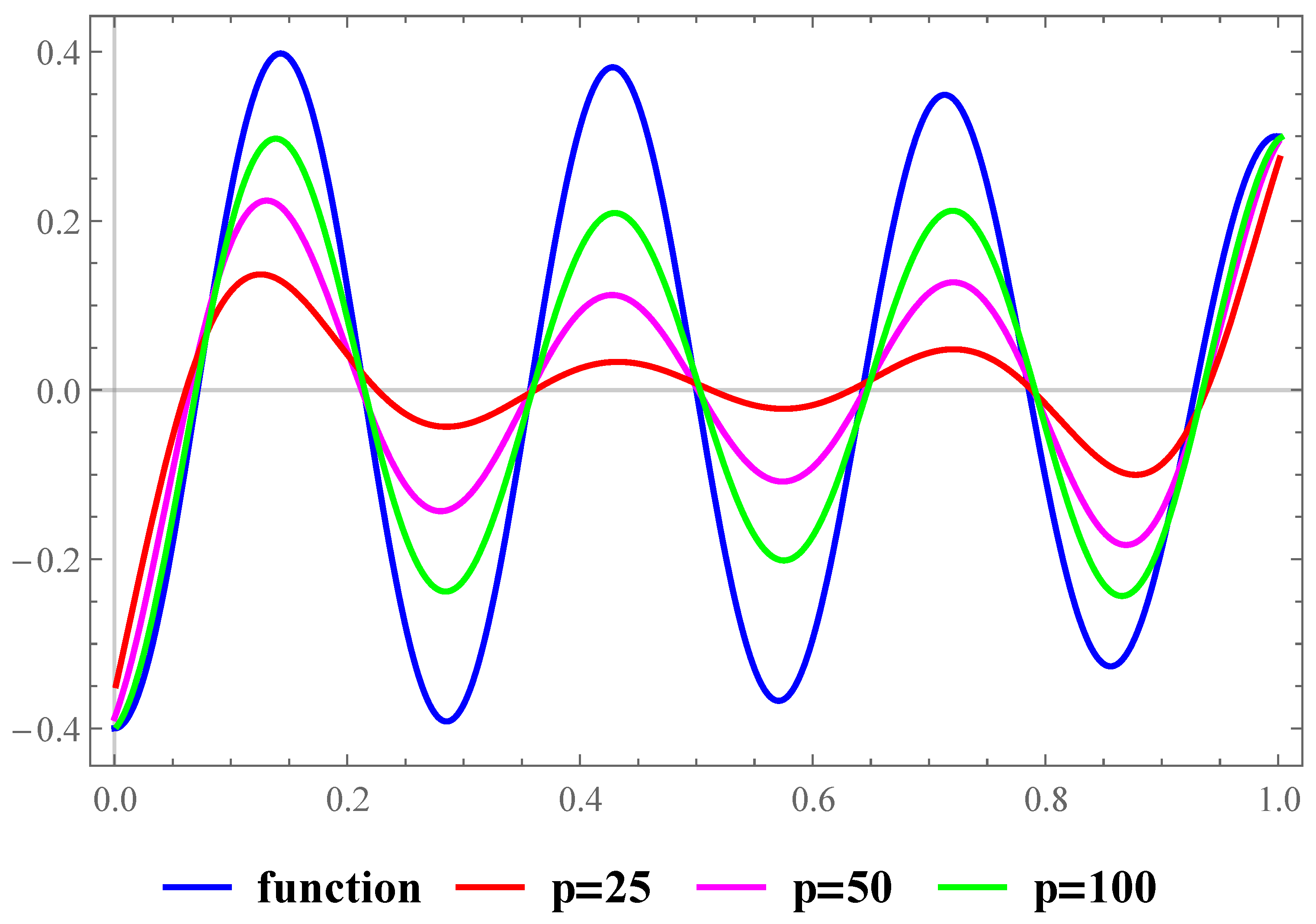
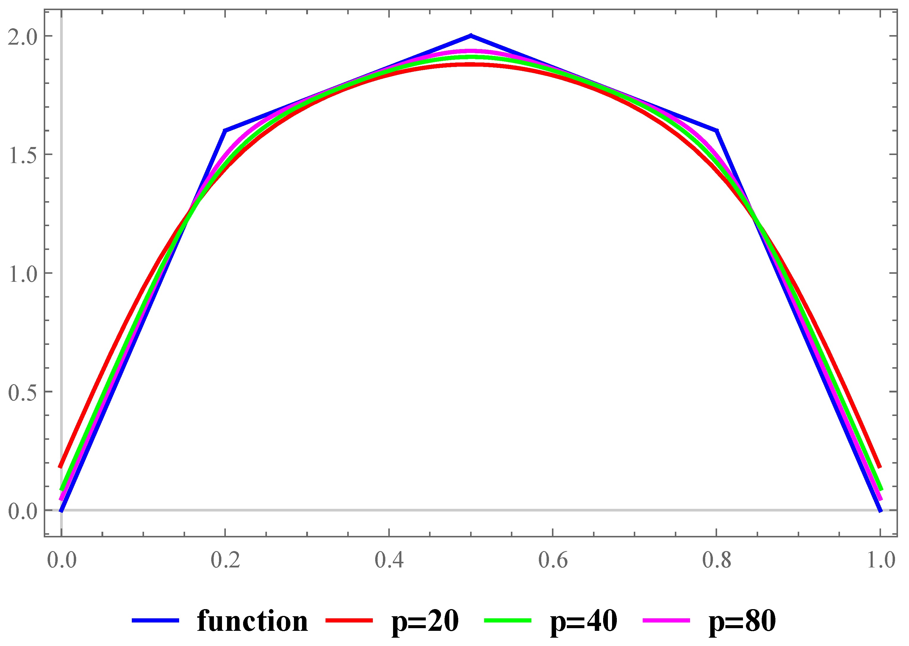
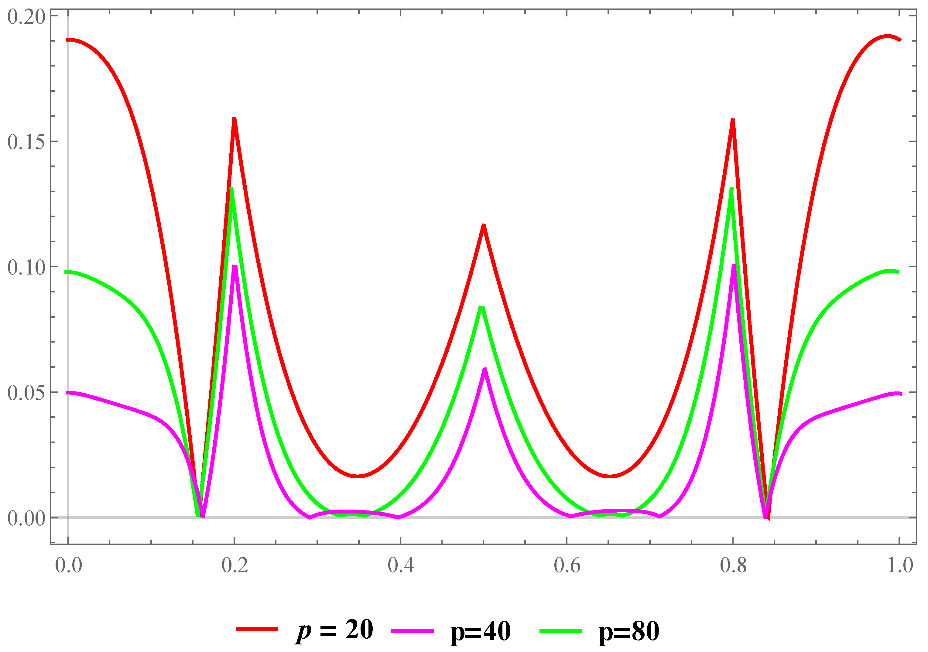
Example 1.

Consider the trigonometric function

$$r_1\left(u\right)=\frac{1}{5}\left(0.5u^2+4\right)sin\left(3\pi u\right)$$

on the closed interval $\mathcal{I}.$ In Figure 1 and Figure 2, we demonstrate approximation and maximum error of approximation of the proposed operators with the values $s=3$, $\alpha =0.9$ and $\lambda =1.$

Figure 1. Approximations by ${\mathcal{K}}_{p,\lambda }^{(\alpha ,s)}$ for function $r_1\left(u\right)$.

Figure 2. Maximum error of approximation for function $r_1\left(u\right)$.

Example 2.

Consider the piece-wise function

$$r_2\left(u\right)=\left\{\begin{array}{cc}8u\hfill & 0\le u\le \frac{1}{5}\hfill \\ \frac{4(1+u)}{3}\hfill & \frac{1}{5}<u\le \frac{1}{2}\hfill \\ \frac{4(2-u)}{3}\hfill & \frac{1}{2}<u\le \frac{4}{5}\hfill \\ 8(1-u)\hfill & \frac{4}{5}<u\le 1\hfill \end{array}\right.$$

on the interval $\mathcal{I}$ (see [38]). In Figure 3 and Figure 4, we fix the values $s=3$, $\alpha =0.9$ and $\lambda =1,$ and change the values of p to see the approximation behavior and maximum error of approximation of the proposed operators.

Figure 3. Approximations by ${\mathcal{K}}_{p,\lambda }^{(\alpha ,s)}$ for function $r_2\left(u\right)$.

Figure 4. Maximum error of approximation for function $r_2\left(u\right)$.

Example 3.

Consider the trigonometric function

$$r_3\left(u\right)=\frac{cos\left(7\pi u\right)}{2.5u^2-10}$$

on the closed interval $\mathcal{I}.$ In Figure 5 and Figure 6, we demonstrate approximation and maximum error of approximation of the proposed operators with certain different values of $s$, α and $\lambda ,$ and the fixed value of $p=20.$

Figure 5. Approximations by ${\mathcal{K}}_{p,\lambda }^{(\alpha ,s)}$ for function $r_3\left(u\right)$.

Figure 6. Maximum error of approximation for function $r_3\left(u\right)$.

Therefore, we demonstrate the consistency and accuracy of convergence behavior for the proposed blending-type operators via certain computer graphics. The graphics show that the proposed operators approximate different kinds of functions for different values of parameters $\lambda$, $\alpha$ and $s.$

7. Conclusions

Many convergence results, including weighted $\mathcal{B}$-statistical, pointwise and weighted convergences, are obtained for the following introduced blending $(\alpha ,\lambda ,s)$-Bernstein–Kantorovich operators:

$$\begin{array}{c}\hfill {\mathcal{K}}_{p,\lambda }^{(\alpha ,s)}(r;u)=(p+1)\sum _{i=0}^p{\tilde{b}}_{p,i}^{\alpha ,s}(\lambda ;u){\int }_{\frac{i}{p+1}}^{\frac{i+1}{p+1}}r\left(t\right)dt\end{array}$$

The proposed operators extend the current literature for certain values of $\lambda$, $\alpha$ and the positive integer $s:$

(i)

If we take $\alpha =1$, $\lambda =0$ and $s=2$, ${\mathcal{K}}_{p,\lambda }^{(\alpha ,s)}$ becomes the classical Kantorovich operators defined in [3].

(ii)

If we take $\alpha =1$ and $s=2$, ${\mathcal{K}}_{p,\lambda }^{(\alpha ,s)}$ becomes the $\lambda –$Kantorovich operators defined in [6,39].

(iii)

If we take $\lambda =0$ and $s=2$, ${\mathcal{K}}_{p,\lambda }^{(\alpha ,s)}$ becomes the $\alpha –$Kantorovich operators defined in [4].

As a continuation of this study, we will focus on a bivariate version of the proposed operators defined in this paper.

References

1. Weierstrass, V.K. Über die Analytische Darstellbarkeit Sogennanter Willkürlicher Functionen Einer Reellen Veränderlichen; Koniglich Preussischen Akademie der Wissenschcaften zu Berlin: Berlin, Germany, 1885; pp. 633–639, 789–805. [Google Scholar]
2. Bernstein, S. Dámonstration du tháorème de weirstrass. Foundeá sur le calcul des probabilitás. Commun. Soc. Math. Kharkow 1912, 13, 1–2. [Google Scholar]
3. Kantorovich, L.V. Sur certains developements suivant les polynomes de la forme de S. Bernstein I, II. Dokl. Akad. Nauk SSSR 1930, 568, 595–600. [Google Scholar]
4. Mohiuddine, S.A.; Özger, F. Approximation of functions by Stancu variant of Bernstein-Kantorovich operators based on shape parameter α. RACSAM 2020, 114, 70. [Google Scholar] [CrossRef]
5. Mohiuddine, S.A.; Ahmad, N.; Özger, F.; Alotaibi, A.; Hazarika, B. Approximation by the parametric generalization of Baskakov-Kantorovich operators linking with Stancu operators. Iran. J. Sci. Technol. Trans. Sci. 2021, 45, 593–605. [Google Scholar] [CrossRef]
6. Özger, F. Weighted statistical approximation properties of univariate and bivariate λ-Kantorovich operators. Filomat 2019, 33, 11. [Google Scholar] [CrossRef]
7. Kanat, K.; Sofyalıoğlu, M. On Stancu type generalization of (p, q)-Baskakov-Kantorovich operators. Commun. Fac. Sci. Univ. Ank. Ser. A1 Math. Stat. 2019, 68, 1995–2013. [Google Scholar] [CrossRef]
8. Kadak, U.; Özger, F. A numerical comparative study of generalized Bernstein-Kantorovich operators. Math. Found. Comput. 2021, 4, 311. [Google Scholar] [CrossRef]
9. Usta, F.; Akyiğit, M.; Say, F.; Ansari, K.J. Bernstein operator method for approximate solution of singularly perturbed Volterra integral equations. J. Math. Anal. Appl. 2022, 507, 125828. [Google Scholar] [CrossRef]
10. Usta, F. Bernstein approximation technique for numerical solution of Volterra integral equations of the third kind. Comput. Appl. Math. 2021, 40, 161. [Google Scholar] [CrossRef]
11. Chen, X.; Tan, J.; Liu, Z.; Xie, J. Approximation of functions by a new family of generalized Bernstein operators. J. Math. Anal. Appl. 2017, 450, 244–261. [Google Scholar] [CrossRef]
12. Özger, F.; Srivastava, H.M.; Mohiuddine, S.A. Approximation of functions by a new class of generalized Bernstein–Schurer operators. RACSAM 2020, 114, 173. [Google Scholar] [CrossRef]
13. Ye, Z.; Long, X.; Zeng, X.M. Adjustment algorithms for Bézier curve and surface. In Proceedings of the 2010 5th International Conference on Computer Science & Education, Hefei, China, 24–27 August 2010. [Google Scholar]
14. Cai, Q.B.; Lian, B.-Y.; Zhou, G. Approximation properties of λ-Bernstein operators. J. Inequal. Appl. 2018, 2018, 61. [Google Scholar] [CrossRef] [PubMed]
15. Aktuğlu, H.; Yashar, Z.S. Approximation of functions by generalized parametric blending-type Bernstein operators. Iran. J. Sci. Technol. Trans. Sci. 2020, 44, 1495–1504. [Google Scholar] [CrossRef]
16. Mohiuddine, S.A.; Kajla, A.; Mursaleen, M.; Alghamdi, M.A. Blending type approximation by τ-Baskakov-Durrmeyer type hybrid operators. Adv. Differ. Equ. 2020, 2020, 467. [Google Scholar] [CrossRef]
17. Özger, F. On new Bezier bases with Schurer polnomials and corresponding results in approximation theory. Commun. Fac. Sci. Univ. Ank. Ser. A1 Math. Stat. 2020, 69, 376–393. [Google Scholar]
18. Srivastava, H.M.; Özger, F.; Mohiuddine, S.A. Construction of Stancu-type Bernstein operators based on Bézier bases with shape parameter λ. Symmetry 2019, 11, 316. [Google Scholar] [CrossRef]
19. Aslan, R. Some approximation results on λ—Szász-Mirakjan-Kantorovich operators, Fundam. J. Math. Appl. 2021, 4, 150–158. [Google Scholar]
20. Cai, Q.B.; Aslan, R. On a New construction of generalized q—Bernstein Polynomials Based on Shape Parameter λ. Symmetry 2021, 13, 1919. [Google Scholar] [CrossRef]
21. Cai, Q.B.; Aslan, R. Note on a new construction of Kantorovich form q—Bernstein operators related to shape parameter λ. Comput. Model. Eng. Sci. 2022, 130, 1479–1493. [Google Scholar] [CrossRef]
22. Ansari, K.J.; Özger, F.; Ödemiş Özger, Z. Numerical and theoretical approximation results for Schurer–Stancu operators with shape parameter λ. Comput. Appl. Math. 2022, 41, 1–18. [Google Scholar] [CrossRef]
23. Srivastava, H.M.; Ansari, K.J.; Özger, F.; Ödemiş Özger, Z. A link between approximation theory and summability methods via four-dimensional infinite matrices. Mathematics 2021, 9, 1895. [Google Scholar] [CrossRef]
24. Özger, F.; Ansari, K.J. Statistical convergence of bivariate generalized Bernstein operators via four-dimensional infinite matrices. Filomat 2022, 36, 507–525. [Google Scholar] [CrossRef]
25. Özger, F.; Demirci, K.; Yıldız, S. Approximation by Kantorovich variant of λ-Schurer operators and related numerical results. In Topics in Contemporary Mathematical Analysis and Applications; CRC Press: Boca Raton, FL, USA, 2021; pp. 77–94. ISBN 9780367532666. [Google Scholar]
26. Gezer, H.; Aktuğlu, H.; Baytunç, E.; Atamert, M.S. Generalized blending type Bernstein operators based on the shape parameter λ. J. Inequal. Appl. 2022, 2022, 1–21. [Google Scholar]
27. Cai, Q.B.; Ansari, K.J.; Temizer Ersoy, M.; Özger, F. Statistical blending-type approximation by a class of operators that includes shape parameters λ and α. Mathematics 2022, 10, 1149. [Google Scholar] [CrossRef]
28. Korovkin, P.P. Linear Operators and Approximation Theory; Hindustan Publishing Corporation: Delhi, India, 1960. [Google Scholar]
29. Bohman, H. On approximation of continuous and of analytic functions. Ark. Math. 1952, 2, 43–56. [Google Scholar] [CrossRef]
30. Kadak, U.; Braha, N.L.; Srivastava, H.M. Statistical weighted B-summability and its applications to approximation theorems. Appl. Math. Comput. 2017, 302, 80–96. [Google Scholar]
31. Kadak, U. Statistical Summability of double sequences by the weighted mean and associated approximation results. In Applied Mathematical Analysis: Theory, Methods, and Applications; Springer: Cham, Switzerland, 2020; pp. 61–85. [Google Scholar]
32. Kolk, E. Matrix summability of statistically convergent sequences. Analysis 1993, 13, 77–84. [Google Scholar] [CrossRef]
33. Stieglitz, M. Eine verallgemeinerung des begriffs der fastkonvergenz. Math. Japon 1973, 18, 53–70. [Google Scholar]
34. Bell, H.T. Order summability and almost convergence. Proc. Am. Math. Soc. 1973, 38, 548–552. [Google Scholar] [CrossRef]
35. Mursaleen, M.; Nasiruzzaman, M.; Srivastava, H.M. Approximation by bicomplex beta operators in compact-disks. Math. Methods Appl. Sci. 2016, 39, 2916–2929. [Google Scholar] [CrossRef]
36. Lenze, B. On Lipschitz-type maximal functions and their smoothness spaces. Indag. Math. 1988, 91, 53–63. [Google Scholar] [CrossRef]
37. DeVore, R.A.; Lorentz, G.G. Constructive Approximation; Springer: Berlin, Germany, 1993. [Google Scholar]
38. Khosravian-Arab, H.; Dehghan, M.; Eslahchi, M.R. A new approach to improve the order of approximation of the Bernstein operators: Theory and applications. Numer. Algorithms 2018, 77, 111–150. [Google Scholar] [CrossRef]
39. Özger, F. Applications of generalized weighted statistical convergence to approximation theorems for functions of one and two variables. Numer. Funct. Anal. Optim. 2020, 41, 1990–2006. [Google Scholar] [CrossRef]
Figure 1. Approximations by K p , λ ( α , s ) for function r 1 ( u ) .
Mathematics 10 02027 g001